Neuronal Network Topology Indicates Distinct Recovery Processes after Stroke

Abstract

Despite substantial recent progress in network neuroscience, the impact of stroke on the distinct features of reorganizing neuronal networks during recovery has not been defined. Using a functional connections-based approach through 2-photon in vivo calcium imaging at the level of single neurons, we demonstrate for the first time the functional connectivity maps during motion and nonmotion states, connection length distribution in functional connectome maps and a pattern of high clustering in motor and premotor cortical networks that is disturbed in stroke and reconstitutes partially in recovery. Stroke disrupts the network topology of connected inhibitory and excitatory neurons with distinct patterns in these 2 cell types and in different cortical areas. These data indicate that premotor cortex displays a distinguished neuron-specific recovery profile after stroke.

Introduction

The brain is a highly distributed system of neural networks (Sporns, 2011). These networks are considered as complex connections characterized by specific topological features, such as hierarchical modularity, high clustering (a measure of connectedness), presence of high degree nodes (high number of pairwise connections between neurons or brain regions) and short path length (an indication of global integration) (Bullmore and Sporns 2009). These features provide a balance between the segregation of information, and its integration, and lead to predictions of optimized connectional architecture in the healthy brain. Brain diseases can be seen as selective disorders of neural networks or neuronal connectivity (Stam 2014).

Ischemic stroke causes focal cell death and substantial disconnection of individual neurons in adjacent and distant brain regions. Human brain imaging studies demonstrate that behavioral deficits occur in functions in these remotely connected regions after stroke, supporting the linkage between connectivity and impairment of motor functions (Urbin et al. 2014; Carter et al., 2010). Among different structures, motor and premotor cortex circuits have a role in the recovery after stroke in both animal models and in humans (Guggisberg et al. 2017; Kantak et al. 2012; Li et al. 2015; Overman et al. 2012). The processes of cortical network connectivity in relation to functional deficits after stroke can be tracked and mapped using advanced 2-photon in vivo imaging that offers high temporal and spatial resolution (Mohajerani et al. 2013; Zhang et al. 2005a). However, most of the previous work that extracted functional maps, at macroscopic or mesoscopic scales (brain-wide coverage in multiple regions), were limited by their sampling of only specific and limited times after stroke. These studies represented a temporally or a spatially constrained snapshot of network connectivity, without tracking the evolving features of neuronal connectivity over time or in specific neuronal populations. Therefore, the functional architecture and plasticity of inhibitory and excitatory cortical neurons at the level of single neurons or local neuronal ensembles in response to the altered brain networks in stroke is not clear. An understanding the cell-specific neuronal network connectivity patterns after stroke and how these changes with recovery will provide insights into mechanisms of recovery that may be tractable for new therapies.

Here, we use a functional connections-based approach through 2-photon in vivo calcium imaging in awake, head-restrained mice before and after stroke to map cortical connectivity in the regions of motor and premotor cortex that mediate recovery. We demonstrate, maps of functional connectivity during motion and nonmotion states, and distinct patterns of functional connection length distribution (CLD) among excitatory and inhibitory neurons. Stroke disrupts the network topology of connected inhibitory and excitatory neurons in motor and premotor cortex in these regions distant from the infarct. At the level of cortical neuron ensembles, our study supports very specific patterns of functional disconnection after stroke, which differ by inhibitory and excitatory neurons and based on cortical areas. The results strongly suggest that there is not a uniform pattern of altered neuronal network function after stroke, but instead distinct alterations in neuronal network topology depending on brain region (premotor or motor) and neuronal cell types (excitatory or inhibitory) and these patterns are associated with functional deficits and recovery.

Materials and Methods

Animals

All experiments were approved by National Institue of Health (NIH) animal protocol and the University of California Los Angeles Chancellor’s Animal Research Committee. The GAD2tm2 (cre) Zjh/J (GAD2Cre mice) were crossed with a reporter mouse B6.CgGt (ROSA) 26Sortm9 (CAG-tdTomato) Hze/J to identify the GAD2 containing inhibitory neurons (GAD2Cre/Ai9Tomato mice) (Supplementary Figs S1A–C and S5). The parent mice in this crossing are homozygotic and all offspring have both alleles. Three-month-old GAD2Cre/Ai9Tomato mice were maintained on a 12 h light/dark cycle with free access to food and water. Animal number was calculated based on previous 2-photon imaging studies (Mohajerani et al. 2013; Stringer et al. 2019). Mice were randomly assigned to group based on random allocation (https://www.randomizer.org/).

Photothrombotic Model of Focal Stroke

Under isoflurane anesthesia (1–1.5% in a 70% N₂O/30% O₂mixture), mice were placed in a stereotactic apparatus, the skull exposed through a midline incision, cleared of connective tissue and dried. A cold light source (KL1500 LCD, Carl Zeiss MicroImaging, Inc.) attached to a 40× objective giving a 1 mm diameter illumination was positioned 1 mm lateral from Bregma, and 0.2 mL of Rose Bengal solution (Sigma; 10 g l − 1 in normal saline, intraperitoneal i.p.) was administered. After 5 min, the brain was illuminated through the intact skull for 15 min (Fig. 1C and Supplementary Fig. S1B).

Figure 1 .

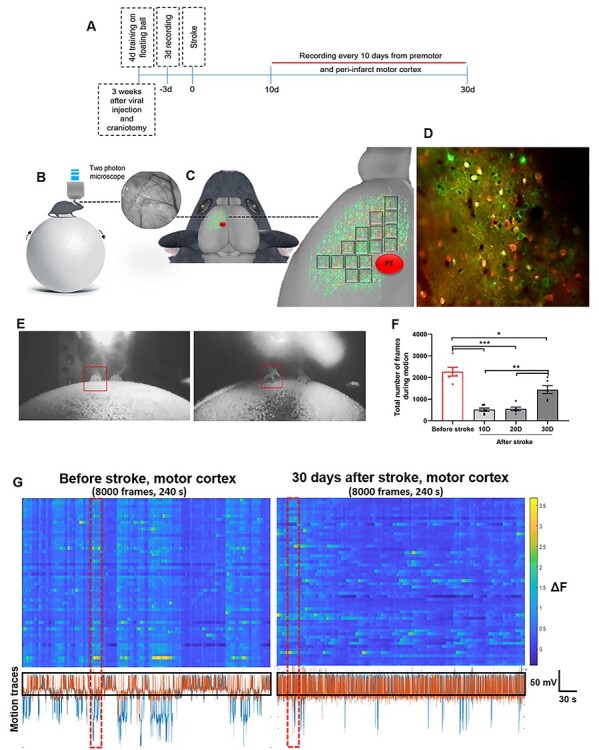
Experimental design and calcium transient properties after stroke. (A) Timeline of the experiment. (B) Left image: showing a head-restrained mouse on the floating ball under 2-photon microscopy. Right image: cranial window of 5 mm through the microscope at 10× covering the green area in C (left image). (C) Left image: schema of GAD2Cre/Ai9Tomato mouse expressing GCaMP6s in motor and premotor cortical neurons, red circle shows the induced stroke (PT) area in motor region. Right image: high magnification of C-left image, indicating recorded regions in motor and premotor cortex. Each gray squares represents a field of view. (D) Average of 8000 frames showing cortical neurons from 1 field of view indicated in C-right image. These motor cortical neurons expressing GCaMP6s (green) in GAD-65 transgenic mice (GAD positive neurons indicating GABAergic inhibitory neurons in red) (E) Images of mouse under 2-photon recording and on the floating ball before and after stroke. Right image shows the affected path locating on the ball after inducing a stroke whereas left image demonstrates animal’s forelimb on the ball before stroke. (F) Total number of frames during motion on the experimental setup before stroke and at different time points after stroke (10, 20, and 30 days). For each session, 8000 frames were recorded. n = 6 mice, data are presented as mean ± SEM. Multiple comparison One-Way ANOVA was applied to compare number of frames with motion at different time points before stoke and with values after stroke. ^*P < 0.05; ^**P < 0.01; ^***P < 0.001; ns, not significant (P > 0.05). (G) Two examples of neuronal firing traces (dF) from 80 neurons in 1 recording session before (left panel) and after stroke (right panel) in motor cortical neurons. Each row represents the neuron’s estimated dF during a session. Lower panels demonstrate the motion signals (mV) on floating ball during trial and black rectangles indicate the threshold for detection of motion (signals below the rectangle are considered as motion) and red rectangles indicate an example of synchronized dF during motion (blue traces indicate moving forward–backward and orange trances indicate moving right-left).

Virus Injections and Craniotomy for Optical Recording

Each mouse received 1 surgery with 3 steps including headbar implantation, virus injection, and craniotomy. Mice were anesthetized with isoflurane (4% v/v for induction and 1–1.25% v/v for maintenance) and head-fixed in a stereotaxic frame. Lidocaine (0.1 mL) was injected under the scalp and the scalp was removed. The skull was then cleaned and the neck muscles were pushed back and glued with super glue and Vetbond. In order to head-restrain the mouse under the 2PLSM (Scientifica), a stainless-steel headbar was fixed with super glue to the base of the skull. For virus injection, a hole in the skull was made with a small steel burr (0.33 mm diameter) for each site of injection. Four sites of injection including 2 sites for motor cortex (~M/L: +1.5 mm, A/P: +1.0 and +1.75 mm) and 2 sites for premotor cortex (M/L: +1 mm, A/P: +2.0 and +2.5 mm for premotor) at 3 depths (400, 300, and 200 μm from dura) were injected with the virus. A Nanoject Microliter Injector (Drummond Scientific Company) with a glass pipette was used to inject 250 nL of GCaMP6s virus (AAV1-Syn-GCaMP6s, AV-1-PV2824 genome copies (GC) mL −1 diluted 1:1 in PBS; University of Pennsylvania vector core, ddTiter: 6.015 × 10¹²) at the rate of 0.02 μL per min. After each injection, the pipette was left in place for at least 15 min to permit the diffusion of the GCaMP6s virus. Craniotomy was performed after 40 min from the last injection. A 5 mm craniotomy was made above the sites of virus injection. The skull was removed and a 5 mm circular glass plate (Warner Instruments) was permanently glued to the skull using Vetbond (Supplementary Fig. S1C). The skull surface and the base of the headbar were then covered with dental acrylic (Ortho-Jet). The animal was given carprofen (5 mg/kg) and amoxicillin (BIOMOX, Virbac Animal Health) postsurgery for at least a week imaging. To verify injection sites, 3 days after completion of recording sessions, mice were deeply anesthetized with isoflurane (4% v/v) and were transcardially perfused with 0.9% saline followed by 10% paraformaldehyde. The brain was then removed and stored in 10% paraformaldehyde. Prior to sectioning, brains were placed in 10% sucrose for 24 h then 50 μm coronal sections were cut at −19 °C using a cryostat and mounted on slides.

Motion Recording

The mouse was positioned in the headbar restrainer and placed under the 2-photon microscopy although its body was positioned on a spherical treadmill composed of an 8 inch Styrofoam ball (Graham Sweet Studios) suspended by compressed air (Fig. 1B–E). The ball could move freely in both the anterior–posterior and lateral directions. Movement of the ball was monitored by optical sensors (Avago Technologies) and collected as voltage readings by a data acquisition system (Analog Devices). Given normal fluctuations in baseline voltage readings from the optical sensors, voltage thresholds were set to detect periods and amounts of motion and nonmotion. For a detailed description of motion detection, see Donzis et al. 2019. In brief, thresholds for detection of motion were determined by identifying the baseline voltage during periods of nonmotion for 6 videos each from 6 different mice and applied to all subsequent recordings. Data from 2 motion sensor channels were combined to determine periods of motion or nonmotion (Fig. 1F and G). A motion epoch was counted if the combined motion lasted for more than 200 ms and ended immediately prior to a sustained period of nonmotion greater than 200 ms. Recording sessions in which an animal displayed motion for the entire session were removed from analysis.

Two-Photon Imaging

Two-photon laser-scanning microscopy was performed with a Moveable Objective Microscope (Sutter MOM) using a Titanium-Sapphire tunable laser (Coherent Ultra II) at 920 nm with 32 kHz resonant scanning and detected with gallium arsenide phosphide (GaAsp) photomultiplier tubes (Hamamatsu), through a 20×0.95 NA water-immersion objective (XLUMPLFL20XW, Olympus). Images were acquired using the ScanImage software (Vidrio Technologies) and processed with ImageJ (NIH). Fully awake mice, without any anesthesia, were mounted on top of a spherical treadmill by securing its headbar onto a custom-made headbar holder under the microscope. The treadmill consisted of a Styrofoam ball resting inside another Styrofoam hollow half-sphere into which a constant stream of compressed air was blown to keep the ball afloat (Graham Sweet, England). The recording sessions were started 3 days before inducing photothrombotic (PT) stroke in the forelimb motor cortex and continued every 10 days and for the duration of 30 days after stroke. GCaMP6s was imaged in the layers 2/3 in peri-infarct motor and premotor cortex before and after inducing stroke. Images were acquired for 8000 frames at 30.82 Hz. The microscope was encased in a light-tight box, and the animals were kept in darkness without visible visual stimuli during the imaging sessions. Before experiments, mice were acclimated to the head fixation and to resting and running on the spherical treadmill, as previously described (Srinivasan et al., 2015).

Data and Statistical Analysis

Recordings were performed from layers II/III of motor and premotor cortical neurons for 8000 frames (30.82 Hz). Calcium imaging videos were analyzed using custom written MATLAB software with NIH ImageJ. First, the videos were visibly inspected to confirm postcorrection image stability and videos with excessive motion artifact or apparent z-shifts were excluded from analysis. Regions of interest (ROIs) corresponding to identifiable cell bodies with an intensity greater than 30% of the background intensity (30×30 pixel window of the darkest region of the video that did not include a neuron or blood vessel) were selected using a semiautomated algorithm. Identified ROIs were eliminated if they were greater than 400 μm² and smaller than 140 μm². Individual neurons were visually rechecked during the initial phase of data analysis and areas that were not obviously somata or filled cell bodies with GCaMP6s over expression were discarded from the data analysis so that analyzed recordings were predominately from cytoplasm of healthy cells and not neuropils. Time traces of fluorescence intensity from the ROIs converted to ΔF/F values as (F(t) − F₀)/F₀. First, the image background as determined by the 30×30 pixel window described above was subtracted from all fluorescent values. The baseline fluorescence, F₀, was then determined as mode value of background subtracted fluorescent values. Ca²⁺ transient peaks were detected by applying a MATLAB smoothing and peak detection function to the waveform. The smoothing function is a standard MATLAB moving average smoothing function. Amplitudes of individual Ca²⁺ transients were calculated as the difference between the peak of a transient and the baseline ΔF/F detected within 49 frames (~1.5 s) prior to the peak to account for any overall drift in the fluorescence. Peaks that were not greater than the root-mean square of the ΔF/F were not considered Ca²⁺ transients. The average amplitudes of the Ca²⁺ transient for a given neuron during motion were determined separately from Ca²⁺ transients occurring during nonmotion (Supplementary Fig. S1D–S). To determine frequency of Ca²⁺ transients, the number of Ca²⁺ transients occurring during either motion or nonmotion was divided by the total time in seconds spent in motion or nonmotion to provide a frequency in Hz (Supplementary Fig. S1D–S).

ΔF/F traces were temporally deconvolved to remove the nonphysiological slow decay in the GCaMP6s signal and sharpen Ca²⁺ transients (Yaksi and Friedrich, 2006; Donzis et al. 2019). In brief, traces were first filtered using a butterworth filter followed by standard MATLAB deconvolution function. For calculating a significant correlation, the deconvolved traces for each cell were correlated to all other cells using a Pearson Product-Moment correlation coefficient. To determine a significant correlation value, we used a Monte Carlo simulation where each deconvolved ΔF/F trace was randomly shifted in time from 0.032 s, the time of a single frame, up to 259.32 s. The time shift only moved the deconvolved ΔF/F values forward in time although any remaining tail of the trace due to the forward time shift was moved to the beginning of the time-shifted trace. The random time shift did not shuffle the sequential order of the Ca²⁺ transients. The shifted trace was then correlated to all other nonshifted deconvolved traces. This random shifting and correlating process was repeated 100 times for each. It is important to note that time points were not exchanged randomly, they were shifted in time with the amount of time shifted randomized (thus, the number of comparisons for average number of 70 neurons per each field of view resulted in 100×69×70 = 483 000 comparisons) (Supplementary Fig. S4 for number of neurons). The 99th percentile of the distribution from the correlation coefficients derived from the Monte Carlo simulation was used as the cutoff for statistically significant Pearson Product-Moment correlation coefficients. Average cutoff for a significant correlation was 0.114 ± 0.003. The proportion of significantly correlated pairs as well as the mean significant Pearson Product-Moment correlation coefficients were calculated (Donzis et al. 2019).

Functional Clustering and Spatiotemporal Neuronal Calcium Activity Analysis

Neuronal activity was normalized such that the peak activity of each neuron’s activity was set to 1, and cross-correlations were calculated for each pairwise combination of neurons (Supplementary Fig. S2). The maximum cross-correlation between each neuron was displayed in a heatmap (Fig. 5A and Supplementary Fig. S3A). Hierarchical clustering of neuronal activity was performed by using each neuron’s pairwise correlations with other neurons as features for clustering. Rather than only considering the maximum cross-correlation between individual neurons, and clustering those with high correlation, we instead considered each neuron’s entire list of pairwise cross-correlations with other neurons and clustered those with similar pairwise correlations with the entire population together. As such neurons with similar pair-wise correlation patterns with other neurons were clustered together. The “linkage” function in MATLAB was used with “complete” linkage (maximum Euclidean distance) between each neuron’s pairwise correlation coefficients. Unique colors were assigned to groups of neurons whose linkage was less than 1.2 and each color represented a neuron cluster. To obtain spatial information for the identified clusters of neurons with similar correlation patterns, each cluster was plotted using their x and y coordinates and colored in accordance with the unique color that was assigned to the cluster during hierarchical clustering (Fig. 5D and Supplementary Fig. S3B). The mean pairwise distance between neurons within the cluster was calculated for each cluster, and pixel units were converted to μM (Fig. 5B, C and Supplementary Fig. S11).

Figure 5 .

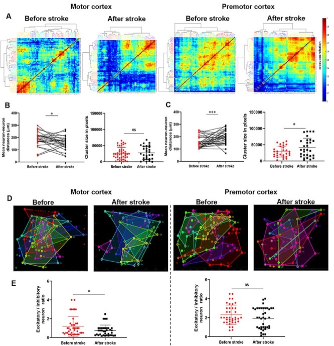
Functional clustering of motor and premotor cortical neurons before and after stroke. (A) Heatmap of pairwise cross-correlation between neuronal activities in motor and premotor cortex for before and after (day 30) stroke periods at motion state. Neurons are ordered by hierarchical clustering as indicate by the dendrogram. Unique colors are assigned to clusters with maximum Euclidean distance <1.2. (B–C) Mean distances between pair of neurons within cluster in motor (B-left, ^*P = 0.0128) and premotor (C-right, ^***P = 0.0002) cortical neurons. Size of cluster in motor (B-right, P = 0.7689) and in premotor (C-right, ^*P = 0.0240) cortical neurons before and after stroke. Size of clusters was calculated in pixels (total size of field of view in pixel: 520×520 = 270 400). (D) Examples for the locations in images of indicated regions of clusters identified by dendrogram colors (panel A). Border color indicates cluster membership; the shaded region indicating the total area covered by neurons within each cluster. Red circles indicate inhibitory neurons and green circles correspond to excitatory neurons. (E) The ratio of excitatory neurons versus inhibitory neurons in motor (left) and premotor (right) cortex before and after inducing stroke. Data are extracted from motion state experiments. n = 5 mice, Error bars indicate SEM. Mann–Whitney U test was used to compare before stroke data with values after stroke. ns, not significant, P > 0.05 and P = 0.1336 for premotor cortex, and ^*P = 0.0287 for motor cortex.

Functional Connectivity and Detecting Edges

In order to identify the functional connectivity, significant Pearson Correlation (PC) obtained from Monte Carlo simulation (99th percentile cutoff) was used to find the threshold. First, the average of significant PC values calculated between each pair of neurons was determined for each session of recording before stroke (). The threshold has been defined as the average value of all calculated for each animal before stroke. The threshold was fix for each mice and was distinct based on the brain areas. This fixed threshold was then used to detect the edges between each pair of neurons before and after stroke. Pair of neurons with higher PC value than threshold was considered functionally connected.

After calculating the functional connectivity, the length of each functional connection was assumed to be the shortest link between spatial positions of 2 connected neurons in a 2D image captured during the recording.

To find the functional CLD, the number of functional connections at different distances from a given neuron was calculated up to 500 μm away from the neuron’s spatial position. For this, the radial distance from a given neuron in network (from 500 μm to 500 μm window of network) was divided into 10 intervals (so that each interval would have 50 μm length). Then the number of valid functional connection between the given neuron and its neighbors at each interval was counted. The result was a vector (CLD) with 10 values in which each value represents the number of edges at certain distance from a given neuron:

Average functional CLD (ACLD) for excitatory or inhibitory neurons was calculated based on the CLD vectors of all neurons in the specified group. ACLD is defined as the average of all CLD vectors in the group:

Statistical tests were run in GraphPad Prism 7.01. Data are presented as mean ± standard mean error (SEM). Note that in some of the graphs, the bars representing the SEM are smaller than the symbols used to represent the mean. For each set of data to be compared, we determined within GraphPad whether the data were normally distributed or not. If they were normally distributed, we used parametric tests; otherwise, we used nonparametric tests. Repeated measures ANOVA and multiple comparisons were used for functional connectivity analyses. For functional CLD, two-way ANOVA and multiple comparisons were applied. Paired and unpaired Student’s two-tailed t tests and Mann–Whitney U test were used for statistical analyses with significance declared at ^*P < 0.05; ^**P < 0.01; ^***P < 0.001; N.S., not significant (P > 0.05).

Results

Adult GAD2Cre/Ai9Tomato male mice which express tdTomato in GABAergic neurons were injected with AAV1.Syn.GCaMP6s.WPRE.SV40 in motor and premotor cortex, to express the high-affinity calcium indictor, GCaMP6s (Fig. 1A–D). All neurons expressed GCaMP6s; inhibitory neurons were differentiated by tdTomato expression (Supplementary Figs S1A, S5 and Video 1). Calcium dynamics were recorded in peri-infarct motor and premotor cortex through a standard cranial window before and after inducing PT stroke in the forelimb motor cortex (Fig. 1B–D and Supplementary Fig. S1A–C). These circuits were chosen because of their demonstrated roles in stroke recovery (Li et al. 2015; Overman et al. 2012), and the lack of neuronal loss in these areas, as they are adjacent to but not within the stroke site (Li et al., 2015) (Supplementary Figs S1B and S12). Furthermore, it has been suggested that motor cortex plays an important role in the functional recovery after motor cortical lesion by enabling downstream circuits to learn and execute specific types of motor skills (Kawai et al. 2015). We first investigated whether freely running on a floating ball can quantify stroke related behavioral deficits and spontaneous motor recovery (Fig. 1E and G). The recording sessions were executed every 10 days for a duration of 30 days after stroke, a time period of spontaneous motor recovery. The number of the frames during the motion state were measured before and after stroke. Mice exhibited a significant decrease in movement at day 10 and 20 after stroke (Fig. 1F). Thirty days after stroke, motion was significantly increased, though still below prestroke levels, indicating partial recovery at this time point (Fig. 1F and G). Other studies indicate that 1 month after stroke is a time period when spontaneous recovery starts (Li et al. 2015; Overman et al. 2012). For these 2 cortical motor areas we analyzed network dynamics by tracking GCaMP6s signals during motion and nonmotion states, with motion analysis inevitably occurring in prestroke and 30-day poststroke time points.

We first asked if elemental physiological properties of excitatory and inhibitory cortical neurons in motor and premotor networks are differentially affected by stroke. We measured the amplitude and frequency of calcium transients in inhibitory and excitatory motor and premotor cortical neurons during motion and nonmotion states, before and 30 days after stroke (Supplementary Fig. S1D–S). Distinct changes in these 2 baseline measurements of neuronal physiological responses were detected after stroke. Both neuronal populations in motor cortex demonstrated reductions in calcium transient amplitude at day 30 after stroke compared with prestroke amplitudes (Supplementary Fig. S1D and F). No changes in amplitude of calcium transient were observed in premotor cortical neurons (Supplementary S1E and G). In addition, excitatory neurons in premotor and motor cortex showed an increase in low frequency calcium transients (Supplementary Fig. S1J and K). These data indicate that stroke causes differential responses in baseline excitability measures in neurons located at motor and premotor areas adjacent to the stroke. In parallel, data obtained from nonstroke control animals demonstrated no change in calcium transient amplitude of excitatory and inhibitory neurons in both structures over periods of recordings (Supplementary Fig. S8). No significant changes were observed for frequency of calcium transient in a control group, except for excitatory neurons of premotor cortex (^*P = 0.305; Supplementary Fig. S7).

Recent studies using macroscopic scale imaging techniques in fMRI demonstrated that stroke functionally disconnects widespread regions of brain and that the disconnection is associated with behavioral deficits (Siegel et al. 2016). Here, at the level of neuronal ensembles, our aim was first, to investigate whether functional disconnectivity after stroke occurs, and second, to study if the functional connectivity of motor or premotor cortical networks are reconfigured as such networks move closer to a more optimal state when spontaneous recovery starts. We applied graph theory-based approaches to measure the functional connectivity of motor or premotor cortex excitatory and inhibitory neuronal networks at a microscopic scale. Same ensembles of neurons were used for analysis at different time points to compare the functional connectivity before and after stroke (see Supplementary Fig. S4 for the number of neurons before and after stroke). Because animals showed little motion at day 10 and 20 after stroke, analysis for the motion state was performed only at day 30 after stroke, to associate dynamics of functional connectivity with behavioral recovery at this time point. Significant correlation values for each pair of neurons were determined using Monte Carlo Simulation on circularly shuffled data at a level of 0.01 and the total number of functional connections for each neuron in the network was calculated.

Stroke diminished functional connectivity for inhibitory and excitatory neuronal populations in motor cortical neurons during the motion state. Before stroke, both neuronal populations show significant correlated firing activity with their neighbors, with excitatory neurons in motor cortex having a higher level of functional connectivity (Figs 2A and 3A). This coordinated activity is greatly reduced after stroke in motor cortex during motion, with a greater reduction in the number of functional connections for inhibitory motor neurons (^*P = 0.0167 for excitatory and ^**P = 0.0022 for inhibitory; Figs 2A and 3A). In parallel, in premotor cortex during motion, a significant decrease in the number of functional connections was observed for excitatory neurons at day 30 after stroke (^*P = 0.0152; Figs 2B and 3A). Interestingly, unlike in motor cortex, the number of functional connections for inhibitory neurons in premotor cortex did not exhibit significant change at 30 days of stroke (P = 0.3095; Figs 2B and 3A). Premotor cortex inhibitory neurons have a normal network connectivity with recovery. Data from the nonstroke control group demonstrated no significant change in motor and premotor cortical neurons during motion at 2 different time points matching the time intervals of the recording days for stroke group (Supplementary Fig. S9).

Figure 2 .

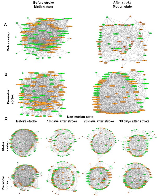
Functional connectome map before and after stroke. (A) Left panel: an example of functional connectivity of motor cortical neurons from 1 mouse before stroke during motion. Right panel: Representing a decrease in number of functional connectivity after stroke for the same neuronal ensemble in A-left panel. (B) Left panel: an example of functional connectivity in premotor cortical neurons before stroke during motion. Right panel: showing functional disconnectivity of B-left network after stroke, only the nodes (neurons with connections) were included in the functional connectome maps, and neurons without connections were exclude here. The green represents excitatory neurons expressing GCaMP6s and the orange circles indicate inhibitory neurons expressing GCaMP6s. The lines connecting the circles (nodes) show the presence of significant functional connectivity between the neurons. Size of circle represents neuron’s degree of connectivity (the larger the circle, the more connected neuron are). (C) Evolution of functional connectivity before stroke and at day 10, 20, and 30 after stroke from nonmotion state data.

Figure 3 .

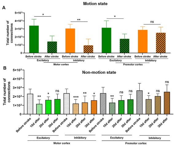
Statistical analysis of functional connectivity before and after stroke. (A) Significant decrease of functional connections demonstrates decrease of correlated activity after stroke during motion. In motor cortex, decrease in number of functional connections after stroke was higher among inhibitory neurons while in premotor cortex number of connections did not decrease 30 days after stroke. (B) Changes in functional connectivity at different time course during nonmotion state. n = 5 mice, data are presented as mean ± SEM. Mann–Whitney U test (for A) and repeated measures ANOVA and multiple comparisons (for B) were used to compare number of connections before stroke with values after stroke. ^*P < 0.05; ^**P < 0.01; ^***P < 0.001; ns, not significant (P > 0.05).

The changes in functional connectivity in motor and premotor cortical networks during the nonmotion state were measured continuously at days 10, 20, and 30 after stroke, because this did not require a behavioral performance. The loss of functional connections between neurons was also observed in the nonmotion state. In motor cortex excitatory neurons, the highest level of reduction in the number of connections was observed 10 days after stroke (^**P = 0.002; Figs 2C and 3B). The functional connection number increased from day 10 to day 20 but it was still lower than the total number of connections before stroke (^*P = 0.0204; Figs 2C and 3B). At day 30 of stroke in the nonmotion state, excitatory neurons of motor cortex did not show a significant decrease in number of total connections compared with before stroke (^*P = 0.0512, Figs 2C and 3B). Stroke caused a loss of functionally linked activity in inhibitory neurons in motor cortex, with an increase in the number of functional connections at successive time points but the level of connectivity 30 days after inducing the stroke was lower than before stroke (D10: ^***P < 0.0007, D20: ^**P = 0.0024 and D30: ^*P = 0.0205). In premotor cortical networks, a recovery in the number of functional connections was observed for both inhibitory and excitatory neurons at day 20 after stroke (D20: P = 0.0521 in excitatory neurons, D20: P = 0.1181 for inhibitory neurons; Figs 2C and 3B). During the nonmotion state, premotor cortical excitatory and inhibitory neurons recovered their functional connectivity earlier than the time of spontaneous motor recovery, whereas in motor cortex only excitatory neurons exhibited recovery at day 30 after stroke when the spontaneous recovery starts (Fig. 3B and Supplementary Table 1).

It is hypothesized that direct and indirect anatomical connections affect robust patterns of functional connectivity and that the wiring costs of these patterns tend to increase with connection distance. The pattern of connection distance among functionally connected networks of the brain may change spontaneously, in response to specific tasks or in response to disease (Bassett and Bullmore, 2017). Having demonstrated that functional connectivity was disrupted by stroke with distinct patterns of functional disconnections in excitatory and inhibitory neurons of motor and premotor cortical networks, we then asked whether stroke affects functional connection distance of neuronal ensembles during the process of spontaneous recovery. The functional connectome, as a connectivity space template based on functional connectivity data in the real physical distribution map of neurons, was defined where nodes (functionally connected neurons) are linked by edges (connections). For each edge, we calculated its connection distance (in micrometers) as the Euclidean distance between the pair of nodes in the standard field of recording space. Based on length distribution data extracted from the motion state, distinct functional connection patterns were identified for motor and premotor cortex neuronal ensembles before stroke and during spontaneous recovery after stroke. In the baseline, nonstroke condition, the strength of functional connectivity between excitatory neurons of motor cortex decays inversely proportional to the physical distance and the majority of edges in the functional network of excitatory neurons have a relatively short distance (between 50 to 250 μm; Fig. 4A, left panel). Stroke disrupts this pattern of connectivity. At day 30 after stroke we observed a significant reduction in the number of short distance functional connections and an increase in the number of long distance functional connections in excitatory neurons in motor cortex (125–175 μm: ^*P = 0.0210 and * = 0.0411, respectively, and ^*P = 0.0324 for 325 μm; Fig. 4A, left panel). Conversely, in motor cortex before stroke, most of the inhibitory neurons exhibited long distance functional connections between 250 μm to 450 μm, whereas the number of inhibitory neurons with short distance functional connections (50–200 μm) was lower. This feature reversed after stroke by an obvious reduction in the number of long distance functional connections and increase in total number of short distance functional connections among inhibitory neurons (125 μm: ^*P = 0.0254 and for 325 to 475 μm, ^*P = 0.0257, ^**P = 0.0099 and ^**P = 0.0054, respectively; Fig. 4B, left panel). Premotor excitatory neurons exhibited the same pattern of functional connectivity as motor cortex in the normal, nonstroke condition, with excitatory neurons forming more short distance functional connections (75–125 μm: ^*P = 0.0295 and ^**P = 0.005, respectively; Fig. 4A, right panel). Similar to motor excitatory neurons, in premotor cortex the number of short distance functional connections decreased after stroke whereas the number of long distance functional connections increased (275 μm: ^*P = 0.0324; Fig. 4B, right panel). However, unlike the inhibitory neurons in motor cortex, inhibitory networks of premotor cortex had a higher number of short distance functional connections compared with a lower number of long distance functional connections before stroke (Fig. 4B, right panel). After stroke, inhibitory neurons preserved their short distance functional connections whereas the number of inhibitory long distance functional connections tended to increase which was against the dynamics of connectivity in the motor cortex inhibitory networks (275–325 μm: ^*P = 0.0128 and ^*P = 0.0458, respectively; Fig. 4B, right panel). These data indicate that stroke reverses normal path distances of network functional connections, except in inhibitory neurons in premotor cortex.

Figure 4 .

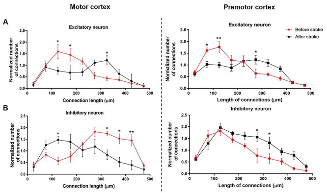
Functional connection distance of inhibitory and excitatory neurons in motor and premotor cortical networks. (A, B) Distribution of functional connection length for excitatory (A) and inhibitory (B) neurons in motor (left panel) and premotor (right panel) cortex. n = 5 mice, data are presented as mean ± SEM. Two-way ANOVA and multiple comparisons were used to compare functional CLD values, before and after stroke. ^*P < 0.05; ^**P < 0.01.

The spatial organization of motor cortex contains distinct functional clustering patterns, measured at macroscopic (Georgopoulos et al. 2007; Amirikian and Georgopoulos 2003) and microscopic scales (Kerr et al. 2007; Dombek et al., 2010). We applied clustering algorithms to determine if neurons could be spatially clustered based on correlations between their temporal activity patterns at the scale of neuronal ensembles (Ozden et al. 2008; Dombek et al., 2010). Data from hierarchical clustering of neuronal activity in the motion state demonstrated a distinct pattern of clustering in motor and premotor cortical ensembles after stroke (Fig. 5A). Using the same ensembles of neurons before and after stroke, we calculated the physical size of each cluster using the number of pixels circumscribed by each cluster of neurons. The size of functionally connected clusters of neurons before and after stroke did not change in motor cortical networks whereas the size of neuronal clusters in premotor cortical ensembles increased at day 30 after stroke (P = 0.7689 and ^*P = 0.0240, respectively; Fig. 5B and C, right panel and Supplementary Fig. S10 for control group). Furthermore, for each cluster, intercluster neuron–neuron connection distances were measured for motor and premotor cortex before and after stroke. Based on collected data in the motion state, the neuron–neuron functional connection distance decreased in the motor cortical neurons after stroke (^*P = 0.0128). However, premotor cortical neurons exhibited a significant increase in neuron–neuron distances after stroke in the motion state (^***P = 0.0002; Fig. 5B and C, Left panel and Supplementary Fig. S11 for control group). Though both premotor and motor cortex are brain areas adjacent to the stroke site, the size of functionally connected neurons and the response to stroke differs substantially between these areas, with the size and distance of connected neuronal ensembles shrinking in motor cortex and expanding in premotor cortex.

Stroke disrupts the excitatory versus inhibitory balance in the brain. It has been shown that an increase in the excitation-to-inhibition ratio (E/I ratio) by pharmacological reduction of GABAergic signaling or enhancing CREB function facilitates plasticity and provides beneficial effects on motor after stroke (Alia et al. 2016; Caracciolo et al. 2018; Clarkson et al. 2010; Murphy and Corbett 2009). Using functional clustering data, we measured the E/I ratio within neuronal clusters in motor and premotor cortex to study the functional balance of active excitatory and inhibitory cortical neurons after stroke (Fig. 5E). For this, we measured the total number of inhibitory and excitatory neurons in each functionally connected cluster from the same ensembles of neurons before and after stroke. These excitatory and inhibitory neurons were functionally active and were clustered because of their correlated activity. The E/I ratio in premotor cortex does not significantly change after 30 days of recovery from stroke (P = 0.1336). However, motor cortical neurons exhibited a significant decrease in the E/I ratio, even at this late time point (^*P = 0.0287). These data suggest that excitatory versus inhibitory balance in premotor cortex regains its functional balance at the onset of spontaneous recovery.

Discussion

Stroke has long been associated with diaschisis, most closely defined as reduced metabolism in distant, connected brain regions after stroke (Carrera and Tononi 2014). The most common example of diaschisis in human is crossed cerebellar diaschisis, although local hypometabolism near a stroke site has also been interpreted as diaschisis (Carmichael et al., 2004). The changes in cortical networks activity after stroke in the present study are not simply a phenomenon of diaschisis or reduced metabolism in brain areas with disconnected neurons. Motor and premotor cortex exhibit different patterns of neuronal activity and functional interactions after stroke. By measuring the correlated activity of neurons in the cortex adjacent to stroke, the present data show that excitatory and inhibitory neurons are, as expected, highly correlated in their activity in premotor and motor cortex in the normal state into functional networks. We follow this pattern of correlated activity or functionally connected networks of neurons over time after stroke in both states of animal motion and nonmotion. During the motion state, a recovery in the number of functionally connected neurons is present only in inhibitory neurons (and not excitatory neurons) of premotor cortex. During the nonmotion state in premotor cortex, recovery in the number of functionally connected neurons occurs for both inhibitory and excitatory neurons, earlier than the time of spontaneous motor recovery. Thirty days after stroke, motor cortex has not recovered in the number of functional connections in both excitatory and inhibitory neuronal ensembles, despite a partial recovery in motor function at this time. Interestingly, during the nonmotion state, only excitatory neuronal ensembles in motor cortex regained their functional connectivity which was correlated with the onset of spontaneous motor recovery and initiation of motion at day 30 after stroke. Data from resting state MRI in humans and rodents demonstrate an increase in intrahemispheric (ipsilesion) functional connectivity at the subacute stage after stroke (weeks after stroke), during the process of motor recovery (Rehme et al. 2015; van Meer et al. 2010). These data were based on the changes in blood-oxygen-level as an indirect way to track brain activity and with lower resolution than single neuron analysis. Our data, at the level of single neurons, with high temporal resolution, indicate for the first time the evolution of functional connectivity in both resting state (nonmotion) and motor performance (here, running on a floating ball) before and after stroke.

We demonstrate that the functional connectivity features in motor and premotor networks after stroke do not change in a unified way and occur differentially based on neuronal subpopulations (inhibitory and excitatory) and behavioral status.

The distance of functional connections within a network defines properties of integration and information transmission. In addition, an inverse relationship is present between node distance and the degree of functional connectivity (Sporns 2011). In brain networks, topological and physical distances between network elements are intricately related. To minimize wiring costs, neurons and brain areas that are spatially close have a high probability of being functionally connected (Averbeck and Seo 2008). In fact, the shortest path between distant nodes (brain areas or neurons) ensures the effective integration and rapid transmission of information (Bullmore and Sporns 2009). We show that excitatory neurons form mainly short distance functional connections and inhibitory neurons of motor cortex display more long distance functional connections in the normal state. Stroke reverses this functional connection distance pattern both in excitatory and inhibitory networks by reducing the long distance correlated firing partners in inhibitory neuronal ensembles of motor cortex and decreasing short distance functional connections in excitatory neurons in both motor and premotor cortex. Furthermore, a specific pattern of functional connection distance distribution among inhibitory neurons of premotor cortical networks emerges over time after stroke, with more long distance functional connections. In parallel to short range, low cost functional connections, brain networks display a small proportion of long, costly functional connections to confer additional performance elements, such as bridges to minimize topological distance between brain regions and facilitate rapid and efficient interareal communication (Bassett and Bullmore, 2017, Betzel and Bassett 2017). Brian disorders affect short and long distance functional connections. Schizophrenic patients exhibit relatively long distances between functionally connected regions and stroke decreases the number of long distance functional connections between brain areas (de Haan et al., 2009, van Meer et al. 2010). Most of these studies were performed at a macroscopic scale and are related to brain areas (with nodes representing brain regions) and not neurons in the networks directly affected in the disease. In contrast, we evaluated the distribution of functional connection distance between nodes at the level of the neuronal ensemble.

In both motor and premotor areas, stroke remodels the distance in which neurons fire in a correlated manner. Interestingly, the inhibitory neurons in premotor cortex take on network properties after stroke that are seen only in motor cortex prior to stroke. In addition, data from functional clustering demonstrate an increase in overall size of the clusters of functionally connected neurons, but only in premotor cortex. This increase in the size of clusters, encompassing all neurons with correlated activity, reflects the formation of bigger microcircuits in premotor cortex. This finding is concomitant with an increase in neuron–neuron connection distances in the premotor cortex. Previous studies, especially data from anatomical mapping, demonstrate that after stroke new and diverse connections in the premotor cortex are formed, due to the axonal sprouting (Li et al. 2015; Omura et al. 2015). The increase in size of neuronal clusters and the mean distances between pairs of neurons in premotor cortex could be explained by the formation of new connections from axonal sprouting, establishing a link between anatomical and functional measures of connectivity. In motor cortex, we observed different responses from premotor cortex, including decreased neuron–neuron connectional distance although the overall size of the neuronal clusters remained stable. This finding of shorter functional connections in motor cortex, but no change in the overall volume of brain that is connected, may preserve crucial microcircuits in this motor cortex after stroke.

An increase in the excitatory versus inhibitory ratio of neurons or in the pattern of activity in a functional brain circuit facilitates plasticity and can be beneficial for motor recovery after stroke (Alia et al. 2016; Clarkson et al. 2010). For example, in the motor cortex adjacent to the focal stroke in the mouse model, there is an increase in tonic GABA inhibition that diminishes recovery (Clarkson et al. 2010). Conversely, enhancing the excitatory signaling adjacent to the stroke region by manipulating molecular systems like CREB phosphorylation, glutamatergic AMPA signaling and CCR5 signaling, enhances recovery (Clarkson et al. 2011; Caracciolo et al. 2018; Joy et al., 2019). The ratio of excitatory versus inhibitory neurons within clusters and in functional cortical networks exhibits different patterns of change in motor and premotor cortex after stroke. One month after stroke, when spontaneous recovery starts, motor cortex still has a reduction in the E/I ratio that could reflect an inhibition in network activity. A decrease in the E/I ratio in the motor cortex can also explain the decrease in correlated activity, disruption in the spatial organization of functionally connected neurons, decrease in neuron-neuron functional distances and smaller cluster size 30 days after stroke. On the other hand, a stable E/I ratio in premotor cortex compared with the prestroke E/I ratio is in accordance with recovered functional connectivity features, increase in neuron–neuron distance and increase in cluster size of the premotor cortical networks.

In summary, in this work we studied features of neuronal network topology at the level of single neurons in motor and premotor cortical networks. We demonstrated whether these specific features exhibit distinct recovery process after stroke, based on the brain areas and the type of neuron. Premotor cortex displayed a distinct neuron-specific recovery profile after stroke; recovery of functional connectivity among inhibitory neurons during motion, full recovery in inhibitory and excitatory neurons during the nonmotion state, and an increase in the cluster size of functionally connected neurons are only observed in premotor cortical networks. These data indicate that recovery in the several features of network topology is present only in premotor cortex. Targeted modulation of excitatory or inhibitory networks in premotor cortex after stroke by using neuromodulation tools like optogenetics and then tracking the cortical networks dynamics by tracking the features of network topology described in this work, can be testable hypothesis for future studies to identify the processes that are engaged in stroke recovery.

Funding

Ressler Family Foundation, the Dr Miriam and Sheldon Adelson Medical Research Foundation, and National Institute of Health R01 NS085019. We also received funding from 1R01NS090930, R01 MH105427, 1R01MH101198 and R01 USPHS NS41574 from National Institute of Health.

Notes

Conflict of Interest: None declared.

References

- Alia C, Spalletti C, Lai S, Panarese A, Micera S, Caleo M. 2016. Reducing GABAA-mediated inhibition improves forelimb motor function after focal cortical stroke in mice. Sci Rep. 6:37823. [DOI] [PMC free article] [PubMed] [Google Scholar]
- Amirikian B, Georgopoulos AP. 2003. Modular organization of directionally tuned cells in the motor cortex: is there a short-range order? Proc Natl Acad Sci U S A. 100(21):12474–12479. [DOI] [PMC free article] [PubMed] [Google Scholar]
- Averbeck BB, Seo M. 2008. The statistical neuroanatomy of frontal networks in the macaque. PLoS Comput Biol. 4(4):e1000050. [DOI] [PMC free article] [PubMed] [Google Scholar]
- Bassett DS, Bullmore ET. 2017. Small-world brain networks revisited. Neuroscientist. 23(5):499–516. [DOI] [PMC free article] [PubMed] [Google Scholar]
- Betzel RF, Bassett DS. 2017. Multi-scale brain networks. Neuroimage. 160: 73–83. doi: 10.1016/j.neuroimage.2016.11.006. [DOI] [PMC free article] [PubMed] [Google Scholar]
- Bullmore E, Sporns O. 2009. Complex brain networks: graph theoretical analysis of structural and functional systems. Nat Rev Neurosci. 10(3):186–198. [DOI] [PubMed] [Google Scholar]
- Caracciolo L, Marosi M, Mazzitelli J, Latifi S, Sano Y, Galvan L, Kawaguchi R, Holley S, Levine MS, Coppola G, et al. 2018. CREB controls cortical circuit plasticity and functional recovery after stroke. Nat Commun. 9(1):2250. [DOI] [PMC free article] [PubMed] [Google Scholar]
- Carmichael ST, Tatsukawa K, Katsman D, Tsuyuguchi N, Kornblum HI. 2004. Evolution of diaschisis in a focal stroke model. Stroke. 35:758–763. [DOI] [PubMed] [Google Scholar]
- Carrera E, Tononi G. 2014. Diaschisis: past, present, future. Brain. 137(PT 9):2408–2422. [DOI] [PubMed] [Google Scholar]
- Carter AR, Astafiev SV, Lang CE, Connor LT, Rengachary J, Strube MJ, Pope DLW, Shulman GL, Corbetta M. 2010. Resting interhemispheric functional magnetic resonance imaging connectivity predicts performance after stroke. Ann Neurol. 67:365–375. doi: 10.1002/ana.21905. [DOI] [PMC free article] [PubMed] [Google Scholar]
- Clarkson AN, Huang BS, Macisaac SE, Mody I, Carmichael ST. 2010. Reducing excessive GABA-mediated tonic inhibition promotes functional recovery after stroke. Nature. 468(7321):305–309. [DOI] [PMC free article] [PubMed] [Google Scholar]
- Clarkson AN, Overman JJ, Zhong S, Mueller R, Lynch G, Carmichael ST. 2011. AMPA receptor-induced local brain-derived neurotrophic factor signaling mediates motor recovery after stroke. J Neurosci. 31(10):3766–3775. [DOI] [PMC free article] [PubMed] [Google Scholar]
- de Haan W, Pijnenburg YA, Strijers RL, van der Made Y, van der Flier WM, Scheltens P, Stam CJ. 2009. Functional neural network analysis in frontotemporal dementia and Alzheimer's disease using EEG and graph theory. BMC Neurosci. 10:101. doi: 10.1186/1471-2202-10-101. [DOI] [PMC free article] [PubMed] [Google Scholar]
- Dombeck D, Harvey C, Tian L, Looger LL, Tank DW. 2010. Functional imaging of hippocampal place cells at cellular resolution during virtual navigation. Nat Neurosci. 13:1433–1440. doi: 10.1038/nn.2648. [DOI] [PMC free article] [PubMed] [Google Scholar]
- Donzis EJ, Estrada-Sánchez AM, Indersmitten T, Oikonomou K, Tran CH, Wang C, Latifi S, Golshani P, Levine MS. 2019. Cortical network dynamics is altered in mouse models of Huntington’s disease. Cereb Cortex. bhz245. doi: 10.1093/cercor/bhz245. [DOI] [PMC free article] [PubMed] [Google Scholar]
- Georgopoulos AP, Merchant H, Naselaris T, Amirikian B. 2007. Mapping of the preferred direction in the motor cortex. Proc Natl Acad Sci U S A. 104(26):11068–11072. [DOI] [PMC free article] [PubMed] [Google Scholar]
- Guggisberg AG, Nicolo P, Cohen LG, Schnider A, Buch ER. 2017. Longitudinal structural and functional differences between proportional and poor motor recovery after stroke. Neurorehabil Neural Repair. 31(12):1029–1041. [DOI] [PMC free article] [PubMed] [Google Scholar]
- Joy MT, Assayag EB, Shabashov-Stone D, Liraz-Zaltsman S, Mazzitelli J, Arenas M, Abduljawad N, Kliper NE, Korczyn AD, Thareja NS et al. 2019. CCR5 is a therapeutic target for recovery after stroke and traumatic brain injury. Cell. 176:1143–1157 e13. [DOI] [PMC free article] [PubMed] [Google Scholar]
- Kantak SS, Mummidisetty CK, Stinear JW. 2012. Primary motor and premotor cortex in implicit sequence learning--evidence for competition between implicit and explicit human motor memory systems. Eur J Neurosci. 36(5):2710–2715. [DOI] [PubMed] [Google Scholar]
- Kawai, R., T, Markman, R. Poddar, A. Dhawale, A.R. Kampff, B.P. Olveczky. 2015. Motor cortex is required for learning but not for executing a motor skill. Neuron 86: 800–812. doi: 10.1016/j.neuron.2015.03.024. [DOI] [PMC free article] [PubMed] [Google Scholar]
- Kerr JN, de Kock, Greenberg DS, Bruno RM, Sakmann B, Helmchen F. 2007. Spatial organization of neuronal population responses in layer 2/3 of rat barrel cortex. J Neurosci. 27(48):13316–13328. [DOI] [PMC free article] [PubMed] [Google Scholar]
- Li S, Nie EH, Yin Y, Benowitz LI, Tung S, Vinters HV, Bahjat FR, Stenzel-Poore MP, Kawaguchi R, Coppola G, et al. 2015. GDF10 is a signal for axonal sprouting and functional recovery after stroke. Nat Neurosci. 18(12):1737–1745. [DOI] [PMC free article] [PubMed] [Google Scholar]
- Mohajerani MH, Chan AW, Mohsenvand M, LeDue J, Liu R, McVea DA, Boyd JD, Wang YT, Reimers M, Murphy TH. 2013. Spontaneous cortical activity alternates between motifs defined by regional axonal projections. Nat Neurosci. 16(10):1426–1435. [DOI] [PMC free article] [PubMed] [Google Scholar]
- Murphy TH, Corbett D. 2009. Plasticity during stroke recovery: from synapse to behaviour. Nat Rev Neurosci. 10(12):861–872. [DOI] [PubMed] [Google Scholar]
- Omura T, Omura K, Tedeschi A, Riva P, Painter MW, Rojas L, Martin J, Lisi V, Huebner EA, Latremoliere A, et al. 2015. Robust axonal regeneration occurs in the injured CAST/Ei mouse CNS. Neuron. 86(5):1215–1227. [DOI] [PMC free article] [PubMed] [Google Scholar]
- Overman JJ, Clarkson AN, Wanner IB, Overman WT, Eckstein I, Maguire JL, Dinov ID, Toga AW, Carmichael ST. 2012. A role for ephrin-A5 in axonal sprouting, recovery, and activity-dependent plasticity after stroke. Proc Natl Acad Sci U S A. 109(33):E2230–E2239. [DOI] [PMC free article] [PubMed] [Google Scholar]
- Ozden I, Lee HM, Sullivan MR, Wang SS. 2008. Identification and clustering of event patterns from in vivo multiphoton optical recordings of neuronal ensembles. J Neurophysiol. 100(1):495–503. [DOI] [PMC free article] [PubMed] [Google Scholar]
- Rehme AK, Volz LJ, Feis DL, Eickhoff SB, Fink GR, Grefkes C. 2015. Individual prediction of chronic motor outcome in the acute post-stroke stage: behavioral parameters versus functional imaging. Hum Brain Mapp. 36(11):4553–4565. [DOI] [PMC free article] [PubMed] [Google Scholar]
- Siegel JS, Ramsey LE, Snyder AZ, Metcalf NV, Chacko RV, Weinberger K, Baldassarre A, Hacker CD, Shulman GL, Corbetta M. 2016. Disruptions of network connectivity predict impairment in multiple behavioral domains after stroke. Proc Natl Acad Sci U S A. 113(30):E4367–E4376. [DOI] [PMC free article] [PubMed] [Google Scholar]
- Sporns O. 2011. The non-random brain: efficiency, economy, and complex dynamics. Front Comput Neurosci. 5:5. [DOI] [PMC free article] [PubMed] [Google Scholar]
- Srinivasan R, Huang BS, Venugopal S, Johnston AD, Chai H, Zeng H, Golshani P, Khakh BS. 2015. Ca(2+) signaling in astrocytes from Ip3r2(−/−) mice in brain slices and during startle responses in vivo. Nat Neurosci. 18:708–717. doi: 10.1038/nn.4001. [DOI] [PMC free article] [PubMed] [Google Scholar]
- Stam CJ. 2014. Modern network science of neurological disorders. Nat Rev Neurosci. 15(10):683–695. [DOI] [PubMed] [Google Scholar]
- Stringer C, Pachitariu M, Steinmetz N, Reddy CB, Carandini M, Harris KD. 2019. Spontaneous behaviors drive multidimensional, brain-wide population activity. Science. 364:255. [DOI] [PMC free article] [PubMed] [Google Scholar]
- Urbin MA, Hong X, Lang CE, Carter AR. 2014. Resting-state functional connectivity and its association with multiple domains of upper-extremity function in chronic stroke. Neurorehabil Neural Repair. 28(8):761–769. [DOI] [PMC free article] [PubMed] [Google Scholar]
- van Meer MP, van der Marel, Wang K, Otte WM, El Bouazati, Roeling TA, Viergever MA, Berkelbach van der Sprenkel JW, Dijkhuizen RM. 2010. Recovery of sensorimotor function after experimental stroke correlates with restoration of resting-state interhemispheric functional connectivity. J Neurosci. 30(11):3964–3972. [DOI] [PMC free article] [PubMed] [Google Scholar]
- Yaksi E, Friedrich RW. 2006. Reconstruction of firing rate changes across neuronal populations by temporally deconvolved Ca2+ imaging. Nat Methods. 3:377–383. doi: 10.1038/nmeth874. [DOI] [PubMed] [Google Scholar]
- Zhang L, Zhang RL, Wang Y, Zhang C, Zhang ZG, Meng H, Chopp M. 2005a. Functional recovery in aged and young rats after embolic stroke: treatment with a phosphodiesterase type 5 inhibitor. Stroke. 36(4):847–852. [DOI] [PubMed] [Google Scholar]
Associated Data
This section collects any data citations, data availability statements, or supplementary materials included in this article.