Effects of stochasticity on the length and behaviour of ecological transients

Abstract

There is a growing recognition that ecological systems can spend extended periods of time far away from an asymptotic state, and that ecological understanding will therefore require a deeper appreciation for how long ecological transients arise. Recent work has defined classes of deterministic mechanisms that can lead to long transients. Given the ubiquity of stochasticity in ecological systems, a similar systematic treatment of transients that includes the influence of stochasticity is important. Stochasticity can of course promote the appearance of transient dynamics by preventing systems from settling permanently near their asymptotic state, but stochasticity also interacts with deterministic features to create qualitatively new dynamics. As such, stochasticity may shorten, extend or fundamentally change a system’s transient dynamics. Here, we describe a general framework that is developing for understanding the range of possible outcomes when random processes impact the dynamics of ecological systems over realistic time scales. We emphasize that we can understand the ways in which stochasticity can either extend or reduce the lifetime of transients by studying the interactions between the stochastic and deterministic processes present, and we summarize both the current state of knowledge and avenues for future advances.

1. Introduction

Two major goals of ecological theory are to make predictions and to explain past observations. In both cases, qualitative changes in dynamics through time represent both a challenge and an opportunity. For prediction, a sudden change in dynamics is important to capture. In parallel, understanding the limits to prediction, in time or in other ways, is important. Both for prediction of the future and for understanding the processes that lead to the current state of the system, the presence of large changes in dynamics [1,2] presents a challenge. How can these events be understood using ecological models?

There is increasing recognition that transients can play a critical role in ecological systems [3–10], building on the variety of long transient behaviours exhibited by nonlinear dynamical systems [11–13]. For example, regime shifts are an important phenomenon in ecology, in which the system behaviour changes suddenly without any warning (e.g. sudden species extinction) [14–16]. The traditional view is that regime shifts are caused by parameter drifting. However, as recently emphasized, even without any parameter change, transient behaviour can lead to regime shifts [8,9].

Earlier work has emphasized the possibility of sudden changes in dynamics even in deterministic models with constant parameters [8], but stochasticity is ubiquitous in real ecosystems and will affect transients [10]. How has the deterministic view limited our understanding of sudden shifts in ecosystems, and how does this understanding deepen when we account for stochasticity in our theoretical constructs and models? This question, in the context of observations of changing ecological dynamics [1,2], fits in with the recent recognition of the importance of focusing on dynamics on ecological time scales. Stochasticity can play an important role in determining dynamics on realistic time scales.

Real-world ecosystems are subject to inevitable and constant influences of stochastic disturbances that can have significant effects on the population dynamics [8,17–31]. A particularly notable example includes the population dynamics of Dungeness crab, Cancer magister, along the West Coast of the USA [32]. In this system, chaotic-like oscillations were analysed using a method that combined data analysis and modelling fitted from data to reveal that the oscillations were actually long transient relaxations due to stochastic perturbations of a stable equilibrium. In addition, random perturbations of cyclic population dynamics can also result in a chaotic-like behaviour, which was observed in the experimental dynamics of Tribolium [33]. Although there have been many individual, well-studied examples illustrating these points, a recognition of common themes arising in a discussion of stochastic transients in ecological systems both reveals new insights into ecological dynamics and suggests important future research directions.

We start from the premise that, in natural systems, noise and random disturbances are inevitable. We consider noise that affects one or more state variables, perturbing them with some magnitude, direction and frequency. Noise can influence long transients in a variety of ways (figure 1). Noise may certainly alter long transient dynamics that were created by another mechanism and already present in the ecological system. Importantly, stochasticity can also provide an alternative mechanism for long transient dynamics, creating a long transient that would not otherwise occur.

Figure 1.

Real-world dynamics fall into the light grey regions, where deterministic and stochastic processes interact. The length and nature of transient dynamics in these regions depend both on the presence of deterministic features known to promote long transients and on properties of the noise. DLT, deterministic long transient (i.e. a long transient that exists in the deterministic part of the dynamics); DST, deterministic short transient. The definition of a ‘long’ transient can be found in §3, and for simplicity we refer to all other transients as ‘short’.

There are two major types of stochasticity in ecological systems: external perturbations due to random variations in the environmental conditions and internal population fluctuations. Environmental stochasticity can sometimes be modelled as additive Gaussian white noise [34,35] or in many cases as multiplicative noise proportional to the population density, while internal stochasticity is effectively demographic noise [24,36–38] that needs to be described as multiplicative noise with its strength depending on the fluctuating abundance variable. Demographic noises are thus correlated, coloured stochastic processes.

We begin this exploration of the role of noise in creating and influencing long transients with some simple examples, illustrating the important point that stochasticity can either extend or reduce transients. Using the simple examples as a jumping-off point, we then undertake a systematic exploration of transients in nonlinear (density-dependent) ecological systems. Even these simple examples bring out the important point that the definition of a transient for a stochastic system may be less clear-cut than for a deterministic one. In particular, we have to be clear about terminology for the case where there is no long transient for the deterministic skeleton of a model, yet the addition of stochasticity produces long-term dynamics that are different from the equilibrium dynamics of the underlying deterministic model. As a way to outline the framework of the current paper, we summarize the current state of synthesis in figure 1. The more systematic approach suggested by this figure first requires attention to the definition of transients and the kinds of stochasticity we consider, followed by different ways in which transients arise and the effects of stochasticity in different cases.

2. Simple examples of transients

Before starting with a systematic exploration of the influence of stochasticity on transients with an emphasis on long transients, simpler systems can provide background. Starting with the simplest case of linear deterministic systems, and then adding stochasticity, will demonstrate first the ecological importance of the phenomena and provide insights into the role of stochasticity.

Age-structured systems provide some of the simplest examples of transient dynamics, which are present even in linear systems. The dynamics of a population of salmon provide a straightforward illustration [39]. Individuals of most salmon species typically reproduce once and then die. In addition, in many populations, almost all individuals reproduce at the same age. We can denote the number of females of age i at time t by n_i(t) in a discrete time description. We assume that the survival from age 1 to age 2 is given by s₁ and similarly by s₂ for age 2 to age 3. Finally, denote the fecundity of 2-year-olds by m₂ with m₂ > 1 and the fecundity of 1- and 3-year-olds by ε₁ and ε₃, respectively, where ε_i ≪ 1. Thus the dynamics of the females would be given by the following Leslie matrix model, if almost all individuals reproduce at age 2:

$$\left(\begin{array}{c}{n}_1(t+1)\\ n_2(t+1)\\ n_3(t+1)\end{array}\right)=\left(\begin{array}{ccc}{ϵ}_1& m_2& {ϵ}_3\\ s_1& 0& 0\\ 0& s_2& 0\end{array}\right)\left(\begin{array}{c}{n}_1(t)\\ n_2(t)\\ n_3(t)\end{array}\right).$$ 2.1

It is easy to see that, if ε₁ = ε₃ = 0, this matrix would have two dominant eigenvalues of the same magnitude. If instead these fecundities are small and positive, then these two eigenvalues would have nearly the same magnitude. In this case, if in a given year almost all individuals were of age 2 and very few were of age 1, then for many years the dominant age class would alternate between 1 and 2. The addition of stochasticity to the return time (i.e. varying the age of reproduction) could greatly reduce the time the system would need to approach stable age distribution (i.e. where the ratio of individuals in different age classes would be constant from year to year).

A second example of a linear ecological transient is given by a simple predator–prey system with an equilibrium that is a stable focus, but with complex eigenvalues with very small, negative real parts. In this case, the deterministic system would have oscillations whose magnitude would decay very slowly, while the presence of environmental stochasticity could extend the time to reach equilibrium [40] by interrupting the decay in cycle magnitudes. Importantly, a similar effect is observed with demographic, as opposed to environmental, stochasticity [41].

What is interesting about these two simple examples is the contrasting effect of stochasticity. In the first one, the Leslie matrix model, clearly stochasticity would shorten the transient by accelerating the approach to the stable age distribution. By contrast, for the predator–prey models, as originally demonstrated [40,42] using Fourier analysis, a stochastic system can continue to exhibit cyclic behaviour indefinitely and thus stochasticity greatly extends the lifetime of the transient, even making it effectively infinite.

If even linear systems can exhibit interesting and contrasting effects of stochasticity on transients, nonlinear systems, which can exhibit longer and more varied kinds of transients [8], will provide a much richer set of phenomena that will be key for ecological understanding. But, before presenting a systematic exploration of long nonlinear transients, it is important to highlight a particular class of stochastic transients which are prominent in ecology and more broadly.

Increasing attention is being paid to tipping points, and early warning signs for tipping based on the concept of critical slowing down have been well studied [43,44]. Critical slowing down refers to the slower return to equilibrium and related phenomena as a bifurcation is approached through parameter change, and thus is related to issues of time scales and therefore transients. Without stochasticity to perturb a system, there would be no opportunity to observe critical slowing down, and thus no possibility of early warning signs. Thus, the concept of critical slowing down has at its core ideas about both transients and stochasticity.

More generally, the concept of critical slowing down can be difficult to apply in practice, as emphasized both from a theoretical [16] and from an empirical [45] standpoint. Though there have been notable and important examples of success in detection of early warning signs in experiments [46,47], much more work is needed to understand this issue. An integration of concepts of stochasticity and transients is one way forward.

An emphasis of early warning sign work has been the detection of parameter changes that push the system through a saddle–node bifurcation. At such a bifurcation, the system’s stable equilibrium is replaced by a ghost attractor which can lead to a long transient [7]. A natural question is how stochasticity affects the length (in time) of a transient resulting from a ghost attractor.

These simple but illustrative examples provide an important starting point for a discussion of transients in stochastic systems. But transients arise in many other ways, and, given the ubiquity of stochasticity, a more thorough and systematic investigation is called for. Clearly, the first steps are an unambiguous definition of transients and a consideration of how stochasticity enters into ecological systems.

3. Definitions of long transients

There are two different ways to define transients in mathematical models (including those with noise) as well as in empirical systems. In this study, we are emphasizing long transients owing to their crucial role in ecological applications including sudden regime shifts. Producing a strict, precise definition of transients is challenging for reasons we note below. We thus view our definition as one that is useful rather than one that is without flaws.

Consider first the scenario where the system is functioning in a certain dynamical regime in which its major characteristics remain unchanged for a long time (for stochastic systems we operate with average characteristics). Here by ‘long time’ we understand the situation where the duration of the regime is much longer than its internal characteristic time (e.g. the period of oscillations). The characteristic time of an ecological system thus depends on the interactions among species. Although not strictly true in an ecological context, this notion of long typically corresponds to a regime duration that is much longer than the generation time of species involved. To the external observer exploring the system based on time series, such a system would appear to be stable. Now suppose that at some moment in time, but without any directional changes to the properties governing the dynamics, the system demonstrates a rapid transition (as compared with the duration of the regime) to another regime, which, in turn, conserves its new characteristics unchanged for a long time again. In this case, we call the preceding dynamical regime a long transient. Note that the post-transitional regime can be transient as well and a new transition may occur later on. In fact, the above-mentioned scenario of transient behaviour describes a shift between regimes. It is also important to emphasize that according to the considered scenario the transition between regimes occurs without external forcing of the system, i.e. without any secular change to model parameters in the course of time. Obviously, however, the presence of the long transient depends on the relationship between the initial conditions and the asymptotic behaviour for the system, so a regime shift due to long transients may be originally triggered by some initial disturbance of either the parameters or the state of the system.

The other long transient scenario involves the situation where the system itself is in slow transition to a stable or quasi-stable state. We assume that the pattern of dynamics evolves very slowly with time as compared with the characteristic time of the current system. For example, this can be the case for damped oscillations with a very long relaxation time where both the amplitude and the period change only slightly. An important practical case is where the transition of the system to the final attractor actually requires an arbitrarily large time [32]. This can happen in the presence of large noise since there will always be perturbations kicking the system away from the eventual asymptotic state. In this case, the resultant pattern of dynamics will be an infinite sequence of transient regimes. We note that calling this behaviour a transient is, perhaps, an arbitrary decision, as the combination of stochasticity plus the deterministic skeleton produces behaviour that persists indefinitely. We believe that this is the more useful choice because it encompasses the role that stochasticity plays in altering dynamics and also note that this provides consistency in our definition.

Another important issue that arises is that any finite population with demographic stochasticity will eventually go extinct. Given this notion, any population is in a transient, which may seem to make the definition too broad. For cases like this, we would suggest that if the addition of stochasticity changes a system from one where the deterministic analogue produces a stable equilibrium and the stochastic version leads to extinction on a time scale too long to be of ecological interest then the transient nature is not the important focus. We view this kind of example as not invalidating our approach, but emphasizing the difficulty of producing a precise definition.

Earlier [9] a key property of long transients was described: there is a scaling law describing the duration of transients while a particular model parameter is varied. The length of a transient regime (in stochastic systems the length should be understood as the mean length) can be made as large as possible when a certain bifurcation parameter (including the magnitude of noise) approaches a critical value. This mathematically quantifies the common-sense notion of ‘long’ transient (i.e. how long is long). From the ecological point of view, the duration of a transient is always limited by natural constraints and we usually assume the average length of transients to be larger than several characteristic generation times [8]. The existence of a scaling law allows us to classify transients into different types [9].

4. Types of noise

In this contribution, we focus primarily on extrinsic temporal noise, that is, those sources of stochasticity that arise because of relationships and quantities external to the modelled system, but also consider demographic stochasticity in some cases. One classic example is detrended environmental variation. Coulson et al. [48] describe active and passive stochasticity, where active noise interacts with deterministic nonlinearity to produce dynamics that cannot result from either factor independently [49], and passive noise influences the transients among different deterministic states. The impact of environmental noise that affects the modelled system will depend on the modelled time frame of interest, the influence of the particular factor, the time scales of variation in the noise relative to the time scales of response and the characteristics of the noise itself.

There are many properties to consider, such as whether the stochasticity is continuous, a single perturbation or seasonal, whether it has larger or smaller magnitude and whether it has frequencies in a similar range to the intrinsic dynamics. Understanding the structure of noise is critical for understanding its potential impact. For example, continuous long-term trended variation such as climate change, short-term uncorrelated variation and directed impacts through management might all be expected to have different effects on the same system.

The most familiar description of environmental stochasticity is as random draws, independent in time, from a Guassian distribution with small variance. In this white noise process, deviations from the mean at one time step are unrelated to the size and magnitude of deviations at another time step. That is, white noise is uncorrelated in time. Or put another way, all frequency components of the signal have the same value. The fact that the variance of noise is small has little bearing on its dynamical impact. To take a trivial case, even small variations close to a critical value in a bifurcation parameter can have a large impact on the dynamics of a system. Environmental stochasticity of relatively small variance can also create oscillations through resonance effects [40,50].

Most environmental signals such as temperature, rainfall and river flow rates have large variance and are autocorrelated in time even after detrending (e.g. [51,52]). The strength of this autocorrelation depends on the signal itself (e.g. air temperature versus sea surface temperature), the geographical location (e.g. continental air temperatures versus maritime air temperatures) and the time period. In particular, climate change is altering the autocorrelation of related environmental signals [53,54]. The autocorrelation of deviations can be large, and, in these cases, can cause clustering of extreme events [55]. Therefore, when we model the impact of environmental stochasticity as a white noise process, we may err in our estimates of the probability of long transient behaviour, as these signals can push a system away from (or towards) an attractor by virtue of the autocorrelated variation.

Patterned noise, for example seasonal forcing [56,57], can have large impacts, and episodic noise (flow-kick) can move and maintain a system far from any attractor in the deterministic scaffold [58].

5. Interactions between stochasticity and transients

The effects of noise on transients are numerous and diverse (figure 1). Noise can make the lifespan of the transient considerably shorter and/or decrease the range of the initial conditions that result in the long transient dynamics, or remove the long transient altogether. Alternatively, noise can make the transient’s lifespan longer. With noise, the emergence of long transient dynamics becomes a probabilistic event rather than a deterministic one. Noise can turn a deterministic long transient into stable, persistent dynamics [40,42]. Moreover, noise can create long transients via mechanisms that do not exist in a deterministic case [59–61].

The outcome of the interaction between noise and a long transient depends both on the properties of noise and on the mechanism behind the (deterministic) long transient. For the transient created by a crawl-by [8] (i.e. caused by the closeness of the system to a saddle point), it is readily seen that uncorrelated noise makes the lifespan of the transient shorter (but does not remove it unless the noise is large), as the random movement of the system in the phase space pushes it, on average, away from the equilibrium. Consequently, the system does not necessarily follow the phase flow along the stable manifold that otherwise would bring it into the close vicinity of the saddle (cf. fig. 2 in [9]). Interestingly, in the presence of noise, long transient dynamics can also emerge, with a certain probability, for a set of initial conditions that would not otherwise lead to a long transient, as the random movement of the system in the phase space can occasionally bring the system into close vicinity of the saddle.

The effect of correlated, directed noise can also make a transient much longer, by keeping the system in the vicinity of a saddle or ghost attractor. In particular, this is readily seen in a flow-kick system [58,62], where the kicks (directed, quasi-periodical, time-discrete random perturbations of the state variable) control the movement of the system over the phase space, with the capacity to keep it close to a specific location in that space (e.g. a saddle or a ghost attractor).

Perhaps the simplest and best-known example where noise can change the system properties qualitatively is the bistable system. We mention here that bistable systems are highly ecologically relevant; in particular, they are used as the paradigm of a regime shift [63] resulting from slow parameter change. Without noise or even with extremely small noise, the system remains in the vicinity of one of the steady states indefinitely long (figure 2a,b). However, slightly larger uncorrelated noise can push the system out of the attraction basin of the current state, so that it rapidly converges to the alternative state: a purely noise-induced regime shift occurs. The dependence of the state variable (e.g. the population size) on time takes the form of alternating periods with a quasi-stationary value (figure 2c). The time spent by the system in the vicinity of the given state increases as the noise intensity decreases and, hence, can be very long. Therefore, small noise creates long transient dynamics. We mention here that there are empirical examples of stochastic switching with long transients in ecological systems [64–66] as well as in epidemiology [67]. Interestingly, noise of larger intensity can destroy the long transient as the system diffuses across the whole span of the phase space between the two states (figure 2d). Therefore, the dependence of the lifetime of the transient dynamics on the strength of noise is non-monotonous. This non-monotonicity is a generic property of population dynamics with stochasticity and is seen in a variety of systems and models (e.g. [68–70]). Below, we see a similar phenomenon emerging in high-dimensional ecological systems.

Figure 2.

Behaviour of a bistable ecological model with different noise levels. In each case, the model with the deterministic skeleton dx/dt = x(x − 0.3)(1 − x) + 0.01, describing the dynamics of a population with scaled population size x describing Allee dynamics, is simulated for different noise levels. The deterministic skeleton is a bistable system where the last term represents a small steady immigration to prevent extinction. The noise term is of the form γxw, where w is a Wiener process (white noise) with mean 0 and variance 1 and the equation is integrated as the equivalent Stratanovich stochastic differential equation using an Euler method and step size of 0.001. Note scale differences. (a) Small noise level, γ = 0.1, starting near the larger equilibrium; system stays near the equilibrium; (b) small noise level, γ = 0.1, starting near the lower equilibrium; system stays near the equilibrium; (c) intermediate noise level, γ = 0.6, showing noise-induced transients; and (d) large noise level, γ = 5, where the system is noise dominated and does not exhibit transients.

Another example of a situation where noise can create long transients is the dynamics of excitable systems [60]. A relevant ecological system that exhibits excitable dynamics is a prey–predator system with Holling type III predation [71]. In a certain parameter range (e.g. where the linear predator nullcline is to the left of the trough of the prey nullcline; see figure 3a), the coexistence state is globally stable, but there is a threshold separating different types of approach to it. For initial conditions on one side of the threshold, the system approaches the steady state directly. For initial conditions on the other, excitable side of the threshold, the system takes an excursion around state space to large abundance of prey and then predator before returning to settle at the steady state. In the deterministic case, once the system has returned to the steady state, it stays there indefinitely. However, the excitability threshold runs close to the steady state, so noise can push the system over the threshold, triggering another large excursion around the phase plane before finally returning to the vicinity of the coexistence state where it can remain for a long time until noise pushes it out again (figure 3b,e). Altogether, the state variable exhibits small-amplitude, random oscillations around the steady-state value intermittent with occasional large-amplitude cycles. An increase in the noise level makes the large-amplitude cycles more frequent; see figures 3c,f. The periods of small-amplitude oscillations are long transients. This dynamic can be viewed as a noise-induced mixed-mode oscillation [72,73].

Figure 3.

Excitable system under the effect of linear additive noise. (a–c) The phase plane of a prey–predator system with Holling type III predation: the irregular red curves show the system trajectories for different levels of noise (increasing from a to b to c), the vertical line is the predator nullcline and the S-shaped curve is the prey nullcline. (d–f) The corresponding dependence of the prey density on time.

Another highly relevant example of transient dynamics facilitated by noise is noise-induced synchronization [61,74]: population oscillations at different locations in space (e.g. in different patches of a fragmented habitat) that would occur asynchronously in the absence of noise can become synchronized under the effect of noise. In ecology, this phenomenon is often referred to as the Moran effect and it is believed to be responsible for masting [75,76]. However, full synchronization only happens when the controlling parameter (e.g. the strength of the noise) exceeds a certain critical value. In the subcritical parameter range, intermittent synchronization occurs, so that the periods of synchronized and asynchronized dynamics alternate [61,77]. In this case, the intervals of synchronized dynamics can be regarded as transients. When the controlling parameter approaches its critical value, their lifetime becomes very long; the average transient time follows the power law [77].

Noise can also turn a transient regime into permanent, sustainable dynamics. As a simple example, let us consider damped population oscillations. In models, such oscillations are frequently observed around a stable focus. Their characteristic life time is $\tau \sim 1/|\text{Re}{\lambda }_0|$, where λ₀ is the eigenvalue with the largest negative real part. Correspondingly, for $|\text{Re}{\lambda }_0|\ll 1$, they last for very long and hence can be regarded as long transient dynamics. The effect of noise can be to turn these long-term damped oscillations into sustained oscillations [40,42,78] through a mechanism known as stochastic resonance [79]. Such quasi-cycles have been reported in several empirical systems, including the dynamics of populations of Dungeness crab [32] and bluefin tuna [80].

As we noted above, tipping points with simple saddle–node bifurcations of equilibria are a core example of the interaction between stochasticity and transients. This interaction becomes even more important with a deterministic system with a chaotic attractor that experiences a crisis [11,12] when its controlling parameter p passes the critical value p_c. Before the bifurcation point, i.e. for p < p_c, there is a chaotic attractor so that chaos is self-sustained; at p = p_c the chaotic attractor turns into a chaotic saddle so that for p > p_c chaotic dynamics are transient. In the presence of chaos, for p > p_c, some, but not all, trajectories may leave the basin of attraction at any given time. The chaotic dynamics that are sustained for the trajectories that remain in the basin instead become transient for the trajectories that leave. The classic three-species food chain [81] is an important ecological example that has this kind of bifurcation. The presence of noise further complicates the situation and can lead to very long transients—supertransients—even for those parameter values where the deterministic system would have a stable chaotic attractor. As previously reviewed [9], in the region where there is deterministic stability, after some time the corresponding stochastic system can cross the basin boundary and leave the basin of attraction for the chaotic attractor and end up in the basin of attraction for a different attractor. This situation is thus a case where stochasticity leads to a transient. A rigorous mathematical analysis of this case is possible [82,83].

6. Systems with positive feedback

There is increasing recognition of the importance of positive feedback in ecological systems [84], and, as figure 2 suggests, stochastic transients are likely to be an important feature of these systems. An important class of systems with positive feedback is mutualistic networks [85–95], e.g. a bipartite network of pollinator and plant species. As a way to illustrate more details about stochastic transients, we describe the analysis of a mutualistic network in more detail. Because the number of species involved in the mutualistic interactions can be large, the system is high dimensional. As is the case in other contexts, much of the dynamical behaviour even in high-dimensional systems can be understood as a phenomenon in low dimensions or one dimension. The distinct dynamical behaviour in complex mutualistic networks is a tipping-point transition, which is codimension 1. In this case, the resulting lower dimensional dynamics are essentially equivalent to the Allee effect.

Consider a complex mutualistic network subject to environmental or demographic noise, or both. The setting thus naturally has high dimensionality and stochasticity. Can transients arise and are they typical? The answer is affirmative. One scenario is tipping-point dynamics [16,43,44,46,47,88,96–104]. In particular, in a mutualistic network, the deterministic behaviour is dominated by the dynamics about a tipping-point transition [92,93]. For example, environmental deterioration will result in massive species extinction, which can occur suddenly in mutualistic systems as a relevant parameter (e.g. the species decay rate) increases through a critical point—a tipping point. Under noise, even when the parameter value has not reached the tipping point, a total system collapse can occur. This is the phenomenon of noise-induced collapse which, dynamically, is nothing but a transition from one steady state to another: from a healthy, high-abundance state to an extinction state. The collapse, of course, does not occur instantaneously: it takes time for the transition to complete, and during this time what we see is a transient. Likewise, when the system is effectively extinct with near-zero species abundances, noise can trigger a recovery of the species abundances. In this case, the transition occurs in the opposite direction: from a low-abundance steady state to a high-abundance one, which is the recently discussed phenomenon of noise-induced recovery [94] accomplished through a transient.

A dynamical picture of the phenomenon of noise-induced collapse and recovery is illustrated in figure 4. In the deterministic case, species collapse and recovery are the result of saddle–node bifurcations. Let κ be the normalized species decay rate (the bifurcation parameter). Environmental deterioration is manifested as an increase in the value of κ. As κ increases through a critical point, denoted as κ_c(0), a reverse saddle–node bifurcation occurs, giving rise to a tipping-point transition. Now consider the case where noise of amplitude ɛ is present. The phenomenon of noise-induced collapse corresponds to an earlier tipping-point transition, now occurring at the critical point κ_c(ɛ), where κ_c(ɛ) < κ_c(0). Likewise, without noise, species recovery occurs through a forward saddle–node bifurcation at κ_r(0), but noise can induce species recovery at a critical point κ_r(ɛ), where κ_r(ɛ) > κ_r(0). For κ_r(0) < κ < κ_c(0), the deterministic system has three equilibria: two stable equilibria and an unstable equilibrium in between. The two stable equilibria are two attractors with their own basins of attraction, while the stable manifold of the unstable equilibrium is the basin boundary [13,105]. Dynamically, the two transition phenomena are the result of noise driving the system across the basin boundary. Transients arise because of the competition between the attractive dynamics in the neighbourhoods of the stable equilibria as controlled by the eigenvalues of the Jacobian matrix with negative real part and stochastic hopping that brings the system out of the attractor [106–108]. The transient dynamics underlying noise-induced collapse and recovery are the result of stochastic forcing that drives the system from one stable steady state to another. For an ensemble of trajectories from random initial conditions, the transient time required for the transition is typically exponentially distributed [109,110] and the average transient lifetime τ depends on the noise amplitude ɛ. For stronger noise, the transition occurs more quickly, so we expect τ to decrease with ɛ. A recent study of four real-world mutualistic networks [111] demonstrated the phenomena of noise-induced collapse and recovery, and confirmed the occurrence of transients.

Figure 4.

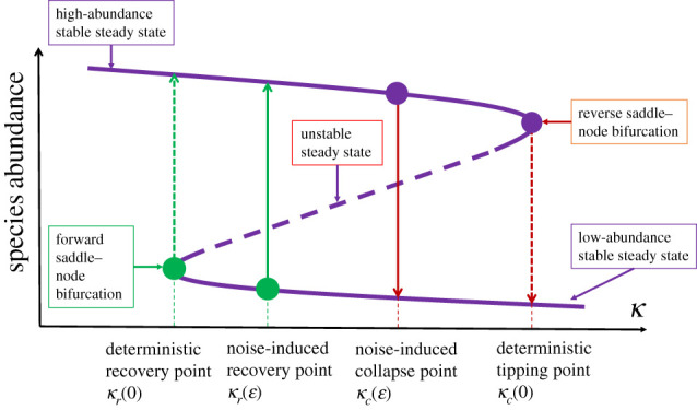
Dynamical mechanism of noise-induced collapse and recovery in mutualistic networks. The bifurcation parameter is the species decay rate κ. The system has two stable steady states, with high and low abundances, respectively. There is an unstable steady state in between the two stable states. The three equilibrium points are dynamically connected through two saddle–node bifurcations: one corresponding to the tipping point (the reverse one) at κ_c(0), and another leading to species recovery (the forward one) at κ_r(0). In the deterministic case, as κ increases through κ_c(0), the system collapses. Under noise of amplitude ɛ, the collapse can occur earlier at κ_c(ɛ)—the phenomenon of noise-induced collapse. Likewise, as κ decreases, noise can induce species recovery at κ_r(ɛ).

It should be noted that the quantities κ_r(ɛ) and κ_c(ɛ) are empirical. Even with noise of arbitrarily small amplitude, sooner or later the system will switch to an alternative steady state, if an infinite amount of observational time is allowed. What is important is whether such a switch can occur on a realistic time scale. Computationally, one can set up a simulation time that is much longer (typically one order of magnitude longer) than any time scale of the system, such as the average time it takes for the system to settle into a steady state from a random initial state. In the presence of noise of amplitude ɛ, one can choose a large number of uniformly spaced values of the decay rate κ and determine the tipping-point transition point κ_c(ɛ) and the noise-induced recovery point κ_r(ɛ).

The common dynamical feature of transition from one stable steady state to another between noise-induced collapse and recovery notwithstanding, the specific nature of the noise does play an important role. In particular, environmental noise is independent of the dynamical variables of the system and is thus simply additive, but demographic noise depends on the species abundances. Before reaching the tipping point where the system is in the high-abundance steady state, demographic noise is weak and environmental noise is the dominant stochastic force to induce a system collapse. By contrast, if the system is in the low-abundance steady state, demographic noise is strong and may lead to extinction. The specific roles played by demographic and environmental noises have implications for devising strategies to manage high-dimensional ecological systems. For example, because of the detrimental role of environmental noise in causing an ecosystem to collapse to a low state, it is imperative to devise methods to reduce the level of environmental noise to keep the system in the healthy state. Conversely, when the system is already close to extinction, a suitable amount of environmental noise may help facilitate recovery [94].

7. Flow-kick dynamics

So far, we have focused on systems where the stochastic influence is due to continual noise. But in real ecological systems there may instead be large disturbances at regular or irregular intervals. These exogenous disturbances may be stochastic or, as in some management settings, they may be tightly controlled. In analyses of transients in a deterministic setting [8,9], the focus is often on the response to a single perturbation of a system away from its asymptotic state. These ideas provide the background behind the approach we use to deal with cases of repeated large disturbances.

Consider a population that—in the absence of noise—has an attracting state. If the system is subject to recurring disturbance by disease, weather extremes, management, etc. it may never even get close to the asymptotic dynamics, but instead will stabilize in a region of state space where the short-term transient dynamics balance the disturbance.

A familiar example is given by fishery management: an undisturbed fish stock might grow to carrying capacity but, when subject to repeated harvesting, does not recover to full carrying capacity between harvests. Indeed, a management strategy typically maintains stock population significantly below carrying capacity to ensure a high recruitment rate and corresponding yield. Alternatively, in the context of an invasive species, the disturbance pattern might represent a culling strategy. In this case, a management strategy of regular removal may be designed to keep the invasive species below a threshold way below carrying capacity.

One approach to exploring this phenomenon mathematically is to combine the growth dynamics of the ecosystem with the disturbance dynamics to define a new system whose asymptotic dynamics represent a balance between growth and disturbance. For example, given a continuous population model $dx/dt=f(x)$ that is repeatedly disturbed by a discrete kick κ to the state variable, the associated flow-kick system (a special case of impulsive differential equations) is defined by the discrete system

$$x_{i+1}=x_i({\tau }_i)+{\kappa }_i,$$ 7.1

for additive disturbance, or

$$x_{i+1}={\kappa }_i{x}_i({\tau }_i),$$ 7.2

for multiplicative disturbance. Here, x(t) is the solution to the undisturbed system with initial condition x, and the ith kick κ_i occurs at time τ_i after the previous kick κ_i−1. In the fishery context, f(x) represents the recruitment function, and the disturbance pattern κ_i, τ_i represents a harvesting strategy. This framework is used in [62] to quantify resilience of ecosystems to regular recurrent disturbances, and in [58] to study the resilience of socially valued properties of natural systems to recurrent disturbance.

This kind of flow-kick system illustrates the essential role played by transient dynamics in the presence of disturbance to yield different qualitative dynamics, in which kicks can move the asymptotic state of the system in any arbitrary way [58]. More formally, given any point x* in n-dimensional state space, and any disturbance time τ, there is a kick κ so that x* is an equilibrium of the flow-kick system (7.1) with κ_i = κ and τ_i = τ for all i. In other words, using a perfectly regular disturbance pattern of fixed kicks at fixed time intervals, one can stabilize the disturbed system anywhere in state space, regardless of the location of attracting sets or basins of attraction of the underlying growth dynamics dx/dt = f(x). This idea can be a very powerful conceptual tool in the management of ecosystems [112].

8. Conclusion

An overarching challenge in understanding the dynamics of ecological systems is to provide insights on ecologically realistic time scales in the presence of both environmental variability and stochasticity driven by small population sizes. In this setting, the asymptotic behaviour of deterministic systems is not relevant, and instead a focus on transient dynamics is required. Examples of transient behaviour have been observed in a variety of ecological systems as previously summarized [8], but a more systematic approach is important for understanding the role of stochasticity in ecological transients, especially in cases where detailed information about the system may be limited. The importance of transients in stochastic systems shows up in a variety of ecological contexts [10] and our contribution here emphasizes both the importance of this phenomenon and the idea that a careful mathematical treatment can find order in what may seem like a series of idiosyncratic examples. This is an area where, despite the advances we have covered here, much more work is needed. For example,the study of transients in spatial systems is obviously important [113,114]. More generally, ecological systems are typically high dimensional and the approach described here provides a guide for future research on these, and related socio-ecological, complex systems.

The work summarized here can also be thought of as an extension to stochastic variation of the insights that come from studying seasonal dynamics [57]. Analyses of seasonal systems have emphasized ecological implications, such as long-term variation of densities and species succession of plankton communities of temperate lakes across the warm season [115], where the random starting conditions play an important role. The existence of transients with time scales much larger than the time of a single season can guarantee the coexistence of many plankton species within a short time period—which would be impossible for a longer period in a constant environment—since the ecosystem is ‘re-set’ each year in a random fashion [116]. In other words, this type of ecological transient seems to be a robust phenomenon; however, mechanisms of observed long transients in many such systems are still unclear owing to the high complexity of communities containing dozens of interacting species, the existence of several time scales and stochastic aspects. Further work based on the ideas we have developed here will shed light on the ecological implications of stochastic transients [10].

Here, we have emphasized using modelled stochastic dynamics as a way to understand and predict real-world dynamics. We might also consider the inverse problem, in which we could think of stochasticity as obscuring the signal of a process of interest. As a result, it is tempting to feel that ecological insights would be improved if we could study ecological systems in isolation from stochastic noise. However, if we could observe ecological dynamics after long times in the absence of noise, we would see one behaviour—the deterministic asymptotic behaviour. In the simplest case, a system at or near its equilibrium would simply sit at equilibrium. If our observations began with the system out of equilibrium, we could see a short transient or part of a long transient eventually approaching the equilibrium. In the presence of noise, however, we have the opportunity to see all of these things within a reasonable observation window, as perturbations push the system from one domain to another [117].

One key example that we have highlighted in this work is unexpected shifts between alternative stable states in ecological systems [43]. Much attention has been focused on single shifts, but many systems move more than once between different states. Important quantities, such as the expected interval between shifts and the proportion of time the system is expected to be in each state, can be computed with knowledge of each stable state’s basin of attraction and the characteristics of the noise. In one dimension, knowledge of the basin of attraction can be obtained from the potential. In higher dimension, surfaces like the quasi-potential [118] or the gradient of a Helmholtz–Hodge decomposition [119] provide analogous information based, respectively, on the most likely path or the average path between basins of attraction. A system that mostly sits at or very near one equilibrium gives us virtually no information about these basins. We may not even know whether other stable states exist in such a system. By contrast, a system that experiences enough stochasticity could shift many times [70].

In conclusion, here we argue that an investigation of noisy nonlinear systems reveals a much richer view of the underlying deterministic structure of ecological systems than does focusing exclusively on unperturbed systems. When we observe a system at equilibrium, we can only infer that the equilibrium exists, not what causes it. When we observe how different parts of the system—such as the population densities of different interacting species—change in response to being in different states or configurations, we gain valuable information about the nonlinearities and feedbacks that are present. Extracting these insights, however, requires a good understanding of how the types of stochasticity present interact with these nonlinearities and feedbacks.

Finally, we emphasize that although we have focused on ecological issues and models here, these themes arise in other areas as well. In particular, interactions between stochasticity and transients are clearly important in neuroscience [120,121], as well as other areas of biology, engineering [122], physics [123] and climate [124].

Data accessibility

This article does not contain any additional data.

Authors' contributions

All authors contributed to conceptualization and writing of the manuscript, with A.H. taking the lead.

Competing interests

We declare we have no competing interests.

Funding

The National Institute for Mathematical and Biological Synthesis is supported by the National Science Foundation through NSF award no. DBI-1300426, with additional support from The University of Tennessee, Knoxville and NSF award no. CCS-1521672. The work of A.H. was also supported by NSF grant no. EF-2025235, and of M.L.Z. by NSF grant no. CCF1522054. S.P. was supported by the RUDN University Strategic Academic Leadership Program.

References

- 1.Anderson SC, Branch TA, Cooper AB, Dulvy NK. 2017. Black-swan events in animal populations. Proc. Natl Acad. Sci. USA 114, 3252-3257. ( 10.1073/pnas.1611525114) [DOI] [PMC free article] [PubMed] [Google Scholar]
- 2.Anderson SC, Ward EJ. 2019. Black swans in space: modeling spatiotemporal processes with extremes. Ecology 100, e02403. ( 10.1002/ecy.2403) [DOI] [PubMed] [Google Scholar]
- 3.Hastings A, Higgins K. 1994. Persistence of transients in spatially structured ecological models. Science 263, 1133-1136. ( 10.1126/science.263.5150.1133) [DOI] [PubMed] [Google Scholar]
- 4.Hastings A. 2001. Transient dynamics and persistence of ecological systems. Ecol. Lett. 4, 215-220. ( 10.1046/j.1461-0248.2001.00220.x) [DOI] [Google Scholar]
- 5.Dhamala M, Lai YC, Holt RD. 2001. How often are chaotic transients in spatially extended ecological systems? Phys. Lett. A 280, 297-302. ( 10.1016/S0375-9601(01)00069-X) [DOI] [Google Scholar]
- 6.Hastings A. 2004. Transients: the key to long-term ecological understanding? Trends Ecol. Evol. 19, 39-45. ( 10.1016/j.tree.2003.09.007) [DOI] [PubMed] [Google Scholar]
- 7.Hastings A. 2016. Timescales and the management of ecological systems. Proc. Natl Acad. Sci. USA 113, 14 568-14 573. ( 10.1073/pnas.1604974113) [DOI] [PMC free article] [PubMed] [Google Scholar]
- 8.Hastings A et al. 2018. Transient phenomena in ecology. Science 361, eaat6412. ( 10.1126/science.aat6412) [DOI] [PubMed] [Google Scholar]
- 9.Morozov A et al. 2020. Long transients in ecology: theory and applications. Phys. Life Rev. 32, 1-40. ( 10.1016/j.plrev.2019.09.004) [DOI] [PubMed] [Google Scholar]
- 10.Shoemaker LG et al. 2020. Integrating the underlying structure of stochasticity into community ecology. Ecology 101, e02922. ( 10.1002/ecy.2922) [DOI] [PMC free article] [PubMed] [Google Scholar]
- 11.Grebogi C, Ott E, Yorke JA. 1982. Chaotic attractors in crisis. Phys. Rev. Lett. 48, 1507-1510. ( 10.1103/PhysRevLett.48.1507) [DOI] [Google Scholar]
- 12.Grebogi C, Ott E, Yorke JA. 1983. Crises, sudden changes in chaotic attractors, and transient chaos. Physica D 7, 181-200. ( 10.1016/0167-2789(83)90126-4) [DOI] [Google Scholar]
- 13.Lai YC, Tél T. 2011. Transient chaos—complex dynamics on finite-time scales. New York, NY: Springer. [Google Scholar]
- 14.Scheffer M, Straile D, van Nes EH, Hosper H. 2001. Climatic warming causes regime shifts in lake food webs. Limnol. Oceanogr. 46, 1780-1783. ( 10.4319/lo.2001.46.7.1780) [DOI] [Google Scholar]
- 15.Carpenter SR et al. 2011. Early warnings of regime shifts: a whole-ecosystem experiment. Science 332, 1079-1082. ( 10.1126/science.1203672) [DOI] [PubMed] [Google Scholar]
- 16.Boettiger C, Hastings A. 2012. Quantifying limits to detection of early warning for critical transitions. J. R. Soc. Interface 9, 2527-2539. ( 10.1098/rsif.2012.0125) [DOI] [PMC free article] [PubMed] [Google Scholar]
- 17.Roughgarden J. 1975. A simple model for population dynamics in stochastic environments. Am. Nat. 109, 713-736. ( 10.1086/283039) [DOI] [Google Scholar]
- 18.Lande R. 1993. Risks of population extinction from demographic and environmental stochasticity and random catastrophes. Am. Nat. 142, 911-927. ( 10.1086/285580) [DOI] [PubMed] [Google Scholar]
- 19.Yao Q, Tong H. 1994. On prediction and chaos in stochastic systems. Phil. Trans. R. Soc. Lond. A 348, 357-369. ( 10.1098/rsta.1994.0096) [DOI] [Google Scholar]
- 20.Ludwig D. 1996. The distribution of population survival times. Am. Nat. 147, 506-526. ( 10.1086/285863) [DOI] [Google Scholar]
- 21.Ripa J, Lundberg P, Kaitala V. 1998. A general theory of environmental noise in ecological food webs. Am. Nat. 151, 256-263. ( 10.1086/286116) [DOI] [PubMed] [Google Scholar]
- 22.Lande R. 1998. Demographic stochasticity and Allee effect on a scale with isotropic noise. Oikos 83, 353-358. ( 10.2307/3546849) [DOI] [Google Scholar]
- 23.Dennis B. 2002. Allee effects in stochastic populations. Oikos 96, 389-401. ( 10.1034/j.1600-0706.2002.960301.x) [DOI] [Google Scholar]
- 24.Bonsall MB, Hastings A. 2004. Demographic and environmental stochasticity in predator–prey metapopulation dynamics. J. Anim. Ecol. 73, 1043-1055. ( 10.1111/j.0021-8790.2004.00874.x) [DOI] [Google Scholar]
- 25.Ellner SP, Turchin P. 2005. When can noise induce chaos and why does it matter: a critique. Oikos 111, 620-631. ( 10.1111/j.1600-0706.2005.14129.x) [DOI] [Google Scholar]
- 26.Lai YC, Liu YR. 2005. Noise promotes species diversity in nature. Phys. Rev. Lett. 94, 038102. ( 10.1103/PhysRevLett.94.038102) [DOI] [PubMed] [Google Scholar]
- 27.Lai YC. 2005. Beneficial role of noise in promoting species diversity through stochastic resonance. Phys. Rev. E 72, 042901. ( 10.1103/PhysRevE.72.042901) [DOI] [PubMed] [Google Scholar]
- 28.Guttal V, Jayaprakash C. 2007. Impact of noise on bistable ecological systems. Ecol. Model. 201, 420-428. ( 10.1016/j.ecolmodel.2006.10.005) [DOI] [Google Scholar]
- 29.Doney SC, Sailley SF. 2013. When an ecological regime shift is really just stochastic noise. Proc. Natl Acad. Sci. USA 110, 2438-2439. ( 10.1073/pnas.1222736110) [DOI] [PMC free article] [PubMed] [Google Scholar]
- 30.Bjornstad ON. 2015. Nonlinearity and chaos in ecological dynamics revisited. Proc. Natl Acad. Sci. USA 112, 6252-6253. ( 10.1073/pnas.1507708112) [DOI] [PMC free article] [PubMed] [Google Scholar]
- 31.O’Regan SM. 2018. How noise and coupling influence leading indicators of population extinction in a spatially extended ecological system. J. Biol. Dyn. 12, 211-241. ( 10.1080/17513758.2017.1339834) [DOI] [PubMed] [Google Scholar]
- 32.Higgins K, Hastings A, Sarvela J, Botsford L. 1997. Stochastic dynamics and deterministic skeletons: population behavior of Dungeness crab. Science 276, 1431-1435. ( 10.1126/science.276.5317.1431) [DOI] [Google Scholar]
- 33.Dennis B, Desharnais RA, Cushing J, Henson SM, Costantino R. 2003. Can noise induce chaos? Oikos 102, 329-339. ( 10.1034/j.1600-0706.2003.12387.x) [DOI] [Google Scholar]
- 34.Heino M. 1998. Noise colour, synchrony and extinctions in spatially structured populations. Oikos 83, 368-375. ( 10.2307/3546851) [DOI] [Google Scholar]
- 35.Benton TG, Lapsley C, Beckerman AP. 2002. The population response to environmental noise: population size, variance and correlation in an experimental system. J. Anim. Ecol. 71, 320-332. ( 10.1046/j.1365-2656.2002.00601.x) [DOI] [Google Scholar]
- 36.Grenfell BT, Bjornstad ON, Finkenstädt BF. 2002. Dynamics of measles epidemics: scaling noise, determinism, and predictability with the TSIR model. Ecol. Monogr. 72, 185-202. ( 10.1890/0012-9615(2002)072[0185:DOMESN]2.0.CO;2) [DOI] [Google Scholar]
- 37.Martín PV, Bonachela JA, Levin SA, Muñoz MA. 2015. Eluding catastrophic shifts. Proc. Natl Acad. Sci. USA 112, E1828-E1836. ( 10.1073/pnas.1414708112) [DOI] [PMC free article] [PubMed] [Google Scholar]
- 38.Constable GWA, Rogers T, McKane AJ, Tarnita CE. 2016. Demographic noise can reverse the direction of deterministic selection. Proc. Natl Acad. Sci. USA 113, E4745-E4754. ( 10.1073/pnas.1603693113) [DOI] [PMC free article] [PubMed] [Google Scholar]
- 39.Botsford LW, White JW, Hastings A. 2019. Population dynamics for conservation. Oxford, UK: Oxford University Press. [Google Scholar]
- 40.Nisbet RM, Gurney W. 1982. Modelling fluctuating populations. New York, NY: Wiley & Sons. [Google Scholar]
- 41.McKane AJ, Newman TJ. 2005. Predator-prey cycles from resonant amplification of demographic stochasticity. Phys. Rev. Lett. 94, 218102. ( 10.1103/PhysRevLett.94.218102) [DOI] [PubMed] [Google Scholar]
- 42.Nisbet R, Gurney W. 1976. A simple mechanism for population cycles. Nature 263, 319-320. ( 10.1038/263319a0) [DOI] [PubMed] [Google Scholar]
- 43.Scheffer M et al. 2009. Early-warning signals for critical transitions. Nature 461, 53-59. ( 10.1038/nature08227) [DOI] [PubMed] [Google Scholar]
- 44.Scheffer M. 2010. Complex systems: foreseeing tipping points. Nature 467, 411-412. ( 10.1038/467411a) [DOI] [PubMed] [Google Scholar]
- 45.Eslami-Andergoli L, Dale P, Knight J, McCallum H. 2015. Approaching tipping points: a focussed review of indicators and relevance to managing intertidal ecosystems. Wetlands Ecol. Manage. 23, 791-802. ( 10.1007/s11273-014-9352-8) [DOI] [Google Scholar]
- 46.Drake JM, Griffen BD. 2010. Early warning signals of extinction in deteriorating environments. Nature 467, 456-459. ( 10.1038/nature09389) [DOI] [PubMed] [Google Scholar]
- 47.Dai L, Vorselen D, Korolev KS, Gore J. 2012. Generic indicators for loss of resilience before a tipping point leading to population collapse. Science 336, 1175-1177. ( 10.1126/science.1219805) [DOI] [PubMed] [Google Scholar]
- 48.Coulson T, Rohani P, Pascual M. 2004. Skeletons, noise and population growth: the end of an old debate? Trends Ecol. Evol. 19, 359-364. ( 10.1016/j.tree.2004.05.008) [DOI] [PubMed] [Google Scholar]
- 49.Nguyen HT, Rohani P. 2008. Noise, nonlinearity and seasonality: the epidemics of whooping cough revisited. J. R. Soc. Interface 5, 403-413. ( 10.1098/rsif.2007.1168) [DOI] [PMC free article] [PubMed] [Google Scholar]
- 50.Alonso D, McKane AJ, Pascual M. 2007. Stochastic amplification in epidemics. J. R. Soc. Interface 4, 575-582. ( 10.1098/rsif.2006.0192) [DOI] [PMC free article] [PubMed] [Google Scholar]
- 51.Király A, Bartos I, Jánosi IM. 2006. Correlation properties of daily temperature anomalies over land. Tellus A: Dyn. Meteorol. Oceanogr. 58, 593-600. ( 10.1111/j.1600-0870.2006.00195.x) [DOI] [Google Scholar]
- 52.Pelletier JD. 1997. Analysis and modeling of the natural variability of climate. J. Clim. 10, 1331-1342. () [DOI] [Google Scholar]
- 53.Lenton TM, Dakos V, Bathiany S, Scheffer M. 2017. Observed trends in the magnitude and persistence of monthly temperature variability. Sci. Rep. 7, 1-10. ( 10.1038/s41598-017-06382-x) [DOI] [PMC free article] [PubMed] [Google Scholar]
- 54.Di Cecco GJ, Gouhier TC. 2018. Increased spatial and temporal autocorrelation of temperature under climate change. Sci. Rep. 8, 1-9. ( 10.1038/s41598-018-33217-0) [DOI] [PMC free article] [PubMed] [Google Scholar]
- 55.Bunde A, Eichner JF, Kantelhardt JW, Havlin S. 2005. Long-term memory: a natural mechanism for the clustering of extreme events and anomalous residual times in climate records. Phys. Rev. Lett. 94, 048701. ( 10.1103/PhysRevLett.94.048701) [DOI] [PubMed] [Google Scholar]
- 56.Vesipa R, Ridolfi L. 2017. Impact of seasonal forcing on reactive ecological systems. J. Theor. Biol. 419, 23-35. ( 10.1016/j.jtbi.2017.01.036) [DOI] [PubMed] [Google Scholar]
- 57.White ER, Hastings A. 2020. Seasonality in ecology: progress and prospects in theory. Ecol. Complex 44, 100867. ( 10.1016/j.ecocom.2020.100867) [DOI] [Google Scholar]
- 58.Zeeman ML, Meyer K, Bussmann E, Hoyer-Leitzel A, Iams S, Klasky IJ, Lee V, Ligtenberg S. 2018. Resilience of socially valued properties of natural systems to repeated disturbance: a framework to support value-laden management decisions. Nat. Resour. Model. 31, e12170. ( 10.1111/nrm.12170) [DOI] [Google Scholar]
- 59.Benzi R, Sutera A, Vulpiani A. 1981. The mechanism of stochastic resonance. J. Phys. A 14, L453-L457. ( 10.1088/0305-4470/14/11/006) [DOI] [Google Scholar]
- 60.Lindner B, Garcia-Ojalvo J, Neiman A, Schimansky-Geier L. 2004. Effects of noise in excitable systems. Phys. Rep. 392, 321-424. ( 10.1016/j.physrep.2003.10.015) [DOI] [Google Scholar]
- 61.Moskalenko OI, Koronovskii AA, Zhuravlev MO, Hramov AE. 2018. Characteristics of noise-induced intermittency. Chaos Solitons Fractals 117, 269-275. ( 10.1016/j.chaos.2018.11.001) [DOI] [Google Scholar]
- 62.Meyer K, Hoyer-Leitzel A, Iams S, Klasky I, Lee V, Ligtenberg S, Bussmann E, Zeeman ML. 2018. Quantifying resilience to recurrent ecosystem disturbances using flow-kick dynamics. Nat. Sustain. 1, 671-678. ( 10.1038/s41893-018-0168-z) [DOI] [Google Scholar]
- 63.Scheffer M, Carpenter S, Foley J, Folke C, Walker B. 2001. Catastrophic shifts in ecosystems. Nature 413, 591-596. ( 10.1038/35098000) [DOI] [PubMed] [Google Scholar]
- 64.Taylor KC, Lamorey G, Doyle G, Alley RB, Grootes P, Mayewski PA, White J, Barlow L. 1993. The ‘flickering switch’ of late Pleistocene climate change. Nature 361, 432-436. ( 10.1038/361432a0) [DOI] [Google Scholar]
- 65.Wang R, Dearing JA, Langdon PG, Zhang E, Yang X, Dakos V, Scheffer M. 2012. Flickering gives early warning signals of a critical transition to a eutrophic lake state. Nature 492, 419-422. ( 10.1038/nature11655) [DOI] [PubMed] [Google Scholar]
- 66.Clements CF, Ozgul A. 2016. Including trait-based early warning signals helps predict population collapse. Nat. Commun. 7, 1-8. ( 10.1038/ncomms10984) [DOI] [PMC free article] [PubMed] [Google Scholar]
- 67.Keeling MJ, Rohani P, Grenfell BT. 2001. Seasonally forced disease dynamics explored as switching between attractors. Physica D 148, 317-335. ( 10.1016/S0167-2789(00)00187-1) [DOI] [Google Scholar]
- 68.Fiasconaro A, Spagnolo B, Boccaletti S. 2005. Signatures of noise-enhanced stability in metastable states. Phys. Rev. E 72, 061110. ( 10.1103/PhysRevE.72.061110) [DOI] [PubMed] [Google Scholar]
- 69.Spalding C, Doering CR, Flierl GR. 2017. Resonant activation of population extinctions. Phys. Rev. E 96, 042411. ( 10.1103/PhysRevE.96.042411) [DOI] [PubMed] [Google Scholar]
- 70.Abbott KC, Dakos V. 2020. Mapping the distinct origins of bimodality in a classic model with alternative stable states. Theor. Ecol. ( 10.1007/s12080-020-00476-5) [DOI] [Google Scholar]
- 71.Morozov AY, Petrovskii SV. 2009. Excitable population dynamics, biological control failure, and spatiotemporal pattern formation in a model ecosystem. Bull. Math. Biol. 71, 863-887. ( 10.1007/s11538-008-9385-3) [DOI] [PubMed] [Google Scholar]
- 72.Borowski P, Kuske R, Li YX, Cabrera JL. 2010. Characterizing mixed mode oscillations shaped by noise and bifurcation structure. Chaos 20, 043117.1-043117.22. ( 10.1063/1.3489100) [DOI] [PubMed] [Google Scholar]
- 73.Desroches M, Guckenheimer J, Krauskopf B, Kuehn C, Osinga H, Wechselberger M. 2012. Mixed-mode oscillations with multiple time scales. Siam Rev. 54, 211-288. ( 10.1137/100791233) [DOI] [Google Scholar]
- 74.Toral R, Mirasso CR, Hernández-Garcıa E, Piro O. 2001. Analytical and numerical studies of noise-induced synchronization of chaotic systems. Chaos 11, 665-673. ( 10.1063/1.1386397) [DOI] [PubMed] [Google Scholar]
- 75.Lyles D et al. 2009. The role of large environmental noise in masting: general model and example from pistachio trees. J. Theor. Biol. 253, 701-713. ( 10.1016/j.jtbi.2009.04.015) [DOI] [PubMed] [Google Scholar]
- 76.Rosenstock T, Hastings A, Koenig W, Lyles D, Brown P. 2011. Testing Moran’s theorem in an agroecosystem. Oikos 120, 1434-1440. ( 10.1111/j.1600-0706.2011.19360.x) [DOI] [Google Scholar]
- 77.Moskalenko O, Koronovskii A, Shurygina S. 2011. Intermittent behavior at the boundary of noise-induced synchronization. Tech. Phys. 56, 1369. ( 10.1134/S1063784211090143) [DOI] [Google Scholar]
- 78.Renshaw E. 1991. Modelling biological populations in space and time. Cambridge, UK: Cambridge University Press. [Google Scholar]
- 79.Gammaitoni L, Hänggi P, Jung P, Marchesoni F. 2009. Stochastic resonance: a remarkable idea that changed our perception of noise. Eur. Phys. J. B 69, 1-3. ( 10.1140/epjb/e2009-00163-x) [DOI] [Google Scholar]
- 80.Bjørnstad ON, Nisbet RM, Fromentin JM. 2004. Trends and cohort resonant effects in age-structured populations. J. Anim. Ecol. 73, 1157-1167. ( 10.1111/j.0021-8790.2004.00888.x) [DOI] [Google Scholar]
- 81.Hastings A, Powell T. 1991. Chaos in a three-species food chain. Ecology 72, 896-903. ( 10.2307/1940591) [DOI] [Google Scholar]
- 82.Do Y, Lai YC. 2004. Extraordinarily superpersistent chaotic transients. Europhys. Lett. 67, 914-920. ( 10.1209/epl/i2004-10142-5) [DOI] [Google Scholar]
- 83.Do Y, Lai YC. 2005. Scaling laws for noise-induced superpersistent chaotic transients. Phys. Rev. E 71, 046208. ( 10.1103/PhysRevE.71.046208) [DOI] [PubMed] [Google Scholar]
- 84.Bertness MD, Callaway R. 1994. Positive interactions in communities. Trends Ecol. Evol. 9, 191-193. ( 10.1016/0169-5347(94)90088-4) [DOI] [PubMed] [Google Scholar]
- 85.Bascompte J, Jordano P, Melián CJ, Olesen JM. 2003. The nested assembly of plant-animal mutualistic networks. Proc. Natl Acad. Sci. USA 100, 9383-9387. ( 10.1073/pnas.1633576100) [DOI] [PMC free article] [PubMed] [Google Scholar]
- 86.Guimaraes PR, Jordano P, Thompson JN. 2011. Evolution and coevolution in mutualistic networks. Ecol. Lett. 14, 877-885. ( 10.1111/j.1461-0248.2011.01649.x) [DOI] [PubMed] [Google Scholar]
- 87.Nuismer SL, Jordano P, Bascompte J. 2013. Coevolution and the architecture of mutualistic networks. Evolution 67, 338-354. ( 10.1111/j.1558-5646.2012.01801.x) [DOI] [PubMed] [Google Scholar]
- 88.Lever JJ, Nes EH, Scheffer M, Bascompte J. 2014. The sudden collapse of pollinator communities. Ecol. Lett. 17, 350-359. ( 10.1111/ele.12236) [DOI] [PubMed] [Google Scholar]
- 89.Rohr RP, Saavedra S, Bascompte J. 2014. On the structural stability of mutualistic systems. Science 345, 1253497. ( 10.1126/science.1253497) [DOI] [PubMed] [Google Scholar]
- 90.Dakos V, Bascompte J. 2014. Critical slowing down as early warning for the onset of collapse in mutualistic communities. Proc. Natl Acad. Sci. USA 111, 17546-17551. ( 10.1073/pnas.1406326111) [DOI] [PMC free article] [PubMed] [Google Scholar]
- 91.Guimaraes PR, Pires MM, Jordano P, Bascompte J, Thompson JN. 2017. Indirect effects drive coevolution in mutualistic networks. Nature 550, 511-514. ( 10.1038/nature24273) [DOI] [PubMed] [Google Scholar]
- 92.Jiang J, Huang ZG, Seager TP, Lin W, Grebogi C, Hastings A, Lai YC. 2018. Predicting tipping points in mutualistic networks through dimension reduction. Proc. Natl Acad. Sci. USA 115, E639-E647. ( 10.1073/pnas.1714958115) [DOI] [PMC free article] [PubMed] [Google Scholar]
- 93.Jiang J, Hastings A, Lai YC. 2019. Harnessing tipping points in complex ecological networks. J. R. Soc. Interface 16, 20190345. ( 10.1098/rsif.2019.0345) [DOI] [PMC free article] [PubMed] [Google Scholar]
- 94.Meng Y, Jiang J, Grebogi C, Lai YC. 2020. Noise-enabled species recovery in the aftermath of a tipping point. Phys. Rev. E 101, 012206. ( 10.1103/PhysRevE.101.012206) [DOI] [PubMed] [Google Scholar]
- 95.Ohgushi T, Schmitz O, Holt RD. 2012. Trait-mediated indirect interactions: ecological and evolutionary perspectives. Cambridge UK: Cambridge University Press. [Google Scholar]
- 96.Scheffer M. 2004. Ecology of shallow lakes. Dordrecht, The Netherlands: Springer Science & Business Media. [Google Scholar]
- 97.Wysham DB, Hastings A. 2010. Regime shifts in ecological systems can occur with no warning. Ecol. Lett. 13, 464-472. ( 10.1111/j.1461-0248.2010.01439.x) [DOI] [PubMed] [Google Scholar]
- 98.Ashwin P, Wieczorek S, Vitolo R, Cox P. 2012. Tipping points in open systems: bifurcation, noise-induced and rate-dependent examples in the climate system. Phil. Trans. R. Soc. A 370, 1166-1184. ( 10.1098/rsta.2011.0306) [DOI] [PubMed] [Google Scholar]
- 99.Lenton TM, Livina VN, Dakos V, van Nes EH, Scheffer M. 2012. Early warning of climate tipping points from critical slowing down: comparing methods to improve robustness. Phil. Trans. R. Soc. A 370, 1185-1204. ( 10.1098/rsta.2011.0304) [DOI] [PMC free article] [PubMed] [Google Scholar]
- 100.Barnosky AD et al. 2012. Approaching a state shift in Earth’s biosphere. Nature 486, 52-58. ( 10.1038/nature11018) [DOI] [PubMed] [Google Scholar]
- 101.Boettiger C, Hastings A. 2013. Tipping points: from patterns to predictions. Nature 493, 157-158. ( 10.1038/493157a) [DOI] [PubMed] [Google Scholar]
- 102.Tylianakis JM, Coux C. 2014. Tipping points in ecological networks. Trends Plant. Sci. 19, 281-283. ( 10.1016/j.tplants.2014.03.006) [DOI] [PubMed] [Google Scholar]
- 103.Lontzek TS, Cai YY, Judd KL, Lenton TM. 2015. Stochastic integrated assessment of climate tipping points indicates the need for strict climate policy. Nat. Clim. Change 5, 441-444. ( 10.1038/nclimate2570) [DOI] [Google Scholar]
- 104.Gualdia S, Tarziaa M, Zamponic F, Bouchaudd JP. 2015. Tipping points in macroeconomic agent-based models. J. Econ. Dyn. Contr. 50, 29-61. ( 10.1016/j.jedc.2014.08.003) [DOI] [Google Scholar]
- 105.McDonald SW, Grebogi C, Ott E, Yorke JA. 1985. Fractal basin boundaries. Physica D 17, 125-153. ( 10.1016/0167-2789(85)90001-6) [DOI] [Google Scholar]
- 106.Poon L, Grebogi C. 1995. Controlling complexity. Phys. Rev. Lett. 75, 4023-4026. ( 10.1103/PhysRevLett.75.4023) [DOI] [PubMed] [Google Scholar]
- 107.Kraut S, Feudel U, Grebogi C. 1999. Preference of attractors in noisy multistable systems. Phys. Rev. E 59, 5253-5260. ( 10.1103/PhysRevE.59.5253) [DOI] [PubMed] [Google Scholar]
- 108.Liu Z, Lai YC, Billings L, Schwartz IB. 2002. Transition to chaos in continuous-time random dynamical systems. Phys. Rev. Lett. 88, 124101. ( 10.1103/PhysRevLett.88.124101) [DOI] [PubMed] [Google Scholar]
- 109.Grebogi C, Ott E, Romeiras F, Yorke JA. 1987. Critical exponents for crisis-induced intermittency. Phys. Rev. A 36, 5365-5380. ( 10.1103/PhysRevA.36.5365) [DOI] [PubMed] [Google Scholar]
- 110.Sommerer JC, Ott E, Grebogi C. 1991. Scaling law for characteristic times of noise-induced crises. Phys. Rev. A 43, 1754. ( 10.1103/PhysRevA.43.1754) [DOI] [PubMed] [Google Scholar]
- 111.Meng Y, Lai YC, Grebogi C. 2020. Tipping point and noise-induced transients in ecological networks. J. R. Soc. Interface 17, 20200645. ( 10.1098/rsif.2020.0645) [DOI] [PMC free article] [PubMed] [Google Scholar]
- 112.Francis TB, Abbott KC, Cuddington K, Gellner G, Hastings A, Lai YC, Morozov A, Petrovskii S, Zeeman ML. 2021. Management implications of long transients in ecological systems. Nat. Ecol. Evol. 5, 1-10. ( 10.1038/s41559-020-01365-0) [DOI] [PubMed] [Google Scholar]
- 113.Bel G, Hagberg A, Meron E. 2012. Gradual regime shifts in spatially extended ecosystems. Theor. Ecol. 5, 591-604. ( 10.1007/s12080-011-0149-6) [DOI] [Google Scholar]
- 114.Villa Martín P, Bonachela JA, Levin SA, Muñoz MA. 2015. Eluding catastrophic shifts. Proc. Natl Acad. Sci. USA 112, E1828-E1836. ( 10.1073/pnas.1414708112) [DOI] [PMC free article] [PubMed] [Google Scholar]
- 115.Jager C, Diehl S, Matauschek C, Klausmeier C, Stibor H. 2008. Transient dynamics of pelagic producer grazer systems in a gradient of nutrients and mixing depths. Ecology 89, 1272-1286. ( 10.1890/07-0347.1) [DOI] [PubMed] [Google Scholar]
- 116.Huisman J, Weissing FJ. 1999. Biodiversity of plankton by species oscillations and chaos. Nature 402, 407-410. ( 10.1038/46540) [DOI] [Google Scholar]
- 117.Boettiger C. 2018. From noise to knowledge: how randomness generates novel phenomena and reveals information. Ecol. Lett. 21, 1255-1267. ( 10.1111/ele.13085) [DOI] [PubMed] [Google Scholar]
- 118.Nolting BC, Abbott KC. 2016. Balls, cups, and quasi-potentials: quantifying stability in stochastic systems. Ecology 97, 850-864. ( 10.1890/15-1047.1) [DOI] [PMC free article] [PubMed] [Google Scholar]
- 119.Strang A. 2020. Applications of the Helmholtz-Hodge decomposition to networks and random processes. PhD thesis, Case Western Reserve University, Cleveland, OH, USA.
- 120.Rabinovich M, Huerta R, Laurent G. 2008. Transient dynamics for neural processing. Science 321, 48-50. ( 10.1126/science.1155564) [DOI] [PubMed] [Google Scholar]
- 121.Palmigiano A, Geisel T, Wolf F, Battaglia D. 2017. Flexible information routing by transient synchrony. Nat. Neurosci. 20, 1014. ( 10.1038/nn.4569) [DOI] [PubMed] [Google Scholar]
- 122.Masri SF, Caffrey JP. 2017. Transient response of a SDOF system with an inerter to nonstationary stochastic excitation. J. Appl. Mech. 84, 041005. ( 10.1115/1.4035930) [DOI] [Google Scholar]
- 123.Šiler M, Ornigotti L, Brzobohatỳ O, Jákl P, Ryabov A, Holubec V, Zemánek P, Filip R. 2018. Diffusing up the hill: dynamics and equipartition in highly unstable systems. Phys. Rev. Lett. 121, 230601. ( 10.1103/PhysRevLett.121.230601) [DOI] [PubMed] [Google Scholar]
- 124.Semenov M, Barrow E. 1997. Use of a stochastic weather generator in the development of climate change scenarios. Clim. Change 35, 397-414. ( 10.1023/A:1005342632279) [DOI] [Google Scholar]
Associated Data
This section collects any data citations, data availability statements, or supplementary materials included in this article.
Data Availability Statement