HOG + CNN Net: Diagnosing COVID-19 and Pneumonia by Deep Neural Network from Chest X-Ray Images

Abstract

Coronavirus disease 2019 in short COVID-19 is a contagious disease caused by coronavirus SARS-CoV-2, which has caused a global pandemic and still infecting millions around the globe. COVID-19 has made an enormous impact on everybody’s day-to-day life. One of the main strengths of COVID-19 is its extraordinary infectious capability. Early detection systems can thus play a big role in curbing the exponential growth of COVID-19. Some medical radiography techniques, such as chest X-rays and chest CT scans, are used for fast and reliable detection of coronavirus-induced pneumonia. In this paper, we propose a histogram of oriented gradients and deep convolutional network-based model that can find out the specific abnormality in frontal chest X-ray images and effectively classify the data into COVID-19 positive, pneumonia positive, and normal classes. The proposed system performed effectively in terms of various performance measures and proved capable as an effective early detection system.

Introduction

Coronaviruses are a group of similar RNA viruses that provoke illness in mammals and birds [1]. They come in many forms and there are a few that are responsible for causing the disease in humans. A worldwide pandemic of respiratory diseases called COVID-19 was caused by the recently recognized coronavirus, SARS-CoV-2 [2]. COVID-19 pandemic caused by novel Coronaviruses has affected almost all the countries on the globe. It first emerged in Wuhan, China on 31 December 2019. Currently, more than 34.8 million people are infected and more than 1 million people are dead (until October 4, 2020) [3]. COVID-19 has been characterized as a pandemic by WHO [4] by 11 March 2020.

COVID-19 is extremely contagious and propagates faster in humans. The symptoms of COVID-19 infection involve fever, cough, dyspnea, headache, body or muscle pain, sore throat, fatigue, loss of savor or smell, congestion or runny nose, nausea or vomiting, and diarrhea [5]. In critical situations, it can cause acute respiratory illness, organ failure, and even death. Despite increased emphasis on social distancing and personal hygiene, COVID-19 infection rates are still increasing.

COVID-19 has adversely affected the entire world, both from an economic perspective as well as from a healthcare perspective. The Healthcare systems are failing around the world to provide necessary services due to the extreme numbers of admitted people infected with COVID-19. This overload in terms negatively affects the overall services received by other emergency patients not affected by COVID-19 [6]. Other problems that are also affecting the already stressed-out healthcare systems are scarcity of personal protective equipment (PPE) for health care personnel, shortage of skilled healthcare personnel, shortage of intensive care units (ICU), and shortage of testing kits for the detection of this virus.

To detect the presence of COVID-19, two types of tests are performed: antibody test and viral test, where the viral test reveals an immediate infraction on the other hand antibody test shows a previous infarction. The antibody test requires several days to complete [7]. In viral tests normally, the presence of COVID-19 can be ensured by detecting viral nucleic acid applying reverse transcription-polymerase chain reaction (RT-PCR) [8]. While RT-PCR has been used to detect COVID-19, it has been found in various studies that its detection accuracy is low. The study [9] conducted by C. Long et al. compared RT-PCR with CT and found 97.2% sensitivity from CT on the other hand RT-PCR obtained 83.3% sensitivity. According to the early reports, the sensitivity of RT-PCR ranges from 37 to 71% and takes about 4–6 h which may not be good enough [10–12]. Besides for point-of-care viral test, it takes less than an hour but several viral tests need to send to a laboratory which takes some days [13]. It is of paramount importance to detect COVID-19-affected persons as early as possible to control the spread of the virus.

Pneumonia is another respiratory disease that shares many common symptoms with COVID-19. Pneumonia is an infection that infects one or both lungs. The air sacks generally fill with purulent material, such as fluid or pus. Physical symptoms of Pneumonia include a cough that may produce yellow, greenish, or bloody mucus, fever with shaking and sweating, chills, shortness of breath, rapid breathing, chest pain, nausea, loss of appetite, fatigue, etc. Pneumonia is a common side effect of various infections caused by a virus, bacteria, fungus, and other organisms. Pneumonia is also caused by acute respiratory syndromes, such as Severe Acute Respiratory Syndrome (SARS) and Middle East Respiratory Syndrome (MERS). As COVID-19 is a SARS disease, pneumonia is a common indicator of the viral COVID-19 infection. However, not everybody who is infected by COVID-19 shows signs of pneumonia. Severe pneumonia can be considered as a symptom of a very serious COVID-19 infection. Thus, detecting pneumonia related to COVID-19 infection from chest X-ray images can have very beneficial applications in fast initial patient screening and severity assessment. It has become very important to distinguish between these two diseases during this pandemic situation for controlling the spread of the COVID-19 virus as well as ensuring appropriate healthcare for patients. However, the existence of the COVID-19 virus in a patient cannot be proved through only a pneumonia test. Severe pneumonia is an indication of only the most serious COVID-19 infection. Others infected by the virus may show symptoms, such as fever, dry cough, shortness of breath, body aches, fatigue, chills, nausea, muscle pain, etc. Various invasive forms of PCR tests are the only tests that can detect COVID-19 infections in all stages.

Nowadays, artificial intelligence is used in various medical diagnosis tasks including medical image classification, where it is playing a vital role in detecting diseases efficiently and effectively [14–16]. AI-based systems are expandable, automatic, effective, and extremely viable in clinical settings. Several AI-based approaches have already been explored to find out the presence of COVID-19 in a person’s body using medical imaging techniques. Imaging techniques, such as CT scans and chest X-ray images, can be very helpful for detection but CT is a costly medical test that requires a devoted room that can further increase the infection rate. Recent work indicates that chest X-ray images can be useful to find out the presence of COVID-19 with remarkable accuracy, low cost, and small test time. Research showed that the most common features in an infected person's chest image are peripheral distribution, bilateral involvement as well as ground-glass opacification (GGO) [17]. These features can be used by an artificial neural network to diagnose COVID-19 and Pneumonia patients fast and efficiently.

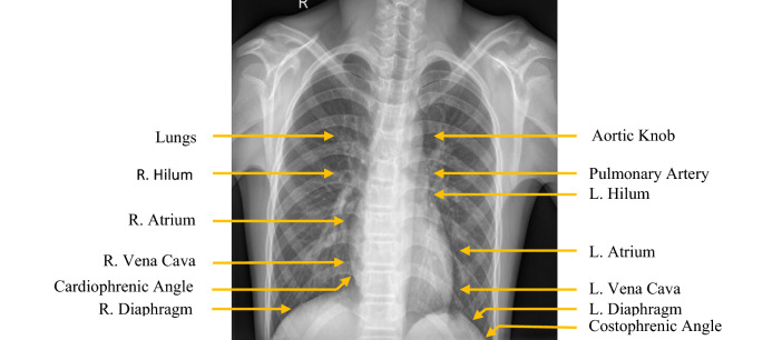
Chest X-ray imaging is a non-invasive, painless, and most commonly performed diagnostic examination for producing images of lungs, heart, airways, blood vessels, and the bones of the spine and chest. In Posterior-Anterior (PA) view, the air is black, bones are white, and the rest of the tissue material falls in between. The majority of the view is filled up by the lung region. As normal lungs are filled with air, the lung regions are relatively darker than the surrounding bones and tissue material. Chest X-ray of normal patients has some other common features, such as sharp costophrenic angles, clearly demarcated hemidiaphragms, sharp borders of heart and other organs, etc. [18]. Figure 1 shows the general anatomy of the chest region of humans from normal PA chest X-ray images.

Fig. 1.

Normal PA chest X-ray demonstrating normal anatomy

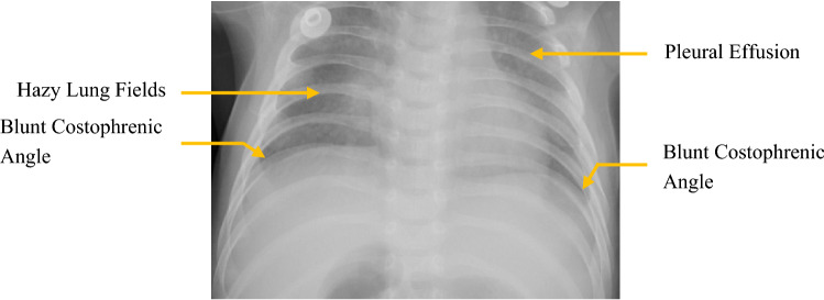
Chest X-rays from patients showing signs of Pneumonia exhibit some of the following features: blunt costophrenic angles showing signs of pleural effusion, white or hazy shadows in the lung fields, hazy border of the heart, and other organs, etc. [19]. Figure 2 shows some of the radiological signs of Pneumonia in PA chest X-ray images.

Fig. 2.

Some symptoms of pneumonia in PA chest X-ray

Many studies have been performed to diagnose pneumonia related to COVID-19 from chest X-ray images. In most of the studies, complex deep learning models were trained directly on X-ray images. This method has some drawbacks, such as relatively high training time based on the complexity of the training data, very high computational cost, the requirement of very powerful computational resources, very high environmental impact based on the complexity of the model, etc.

In this paper, we present a novel method for identifying three types of conditions: COVID-19 induced pneumonia, viral or bacterial pneumonia, and normal patients from chest CT X-ray images. We only extracted useful features from the chest X-ray images by a feature extractor named Histogram of Oriented Gradients (HOG) and trained a custom Convolutional Neural Network (CNN) model on the extracted features. HOG is a feature descriptor widely used in computer vision and image processing applications. While used with a machine learning algorithm, HOG can be used to perform very complex detection and recognition tasks. Thus, this process has several advantages over the traditional deep learning models:

1. The training time is faster than training deep neural networks on images, as images contain a lot of redundant non-important information.

2. The computational cost and the computational resources needed to train the systems are less.

3. The environmental footprint of training such models is also less.

The rest of this paper is organized as follows. “Related Works” outlines an analysis of recently published literature relevant to this study. In “System Overview” a brief description of the system is presented. The overall methodology with data set collection and all the components of the proposed HOG + CNN model is presented in “Methodology”. “Result Analysis” analyzes the performance of the model based on different matrices. Finally, “Conclusion” concludes the literature.

Related Works

AI researchers and data scientists all over the world are introducing various latest technologies to tackle the ongoing COVID-19 pandemic. Many studies propose techniques to diagnose COVID-19 and pneumonia patients using chest X-ray and CT images. These technologies are easy to implement in the medical system and show remarkable performance in diagnosing COVID-19 and pneumonia patients. These technologies can diagnose very fast compared to other conventional methods. Some of the promising works in this field are described as follows.

Razzak et al. [20] developed a system that identifies COVID-19 among healthy cases, bacterial pneumonia, viral pneumonia, where they used transfer learning and compared perfection among CNN architectures. In this study chest X-ray and CT images are used. The data set contains 200 images of COVID-19-affected persons, 200 images of viral pneumonia, 200 images of bacterial pneumonia, and 200 images of normal persons. tenfold cross-validation is used to evaluate the performance of the proposed model. The MobileNet architecture showed 80.95% accuracy for four class classification. Asif and Wenhui [21] focused on categorizing COVID-19 and pneumonia patients by investigating chest X-ray images. They applied the transfer learning approach using DeepCNN-based Inception V3 architecture. They used a chest X-ray data set containing 864 COVID-19-affected images, 1345 viral pneumonia images, and 1341 normal chest X-ray images. The proposed model showed 96% accuracy in the testing phase. Pathari and Rahul [22] proposed an automatic system for detecting COVID-19 and pneumonia, where they used MobileNet V3 neural network architecture. This study analyzes the data of viral pneumonia, Bacterial Pneumonia, COVID-19, and normal cases. The data set contains 24,096 chest X-ray images for training and 3615 chest X-ray images for the testing phase. The transfer learning technique used in this study showed 95.58% accuracy, 97.52% sensitivity, and 95.14% specificity. Makris et al. [23] evaluated fine-tuned convolutional neural networks with transfer learning for detection of COVID-19 from chest X-ray images, where the models are VGG19, VGG16, MobileNetV2, Xception, InceptionV3, ImceptionResNetV2, ResNet152V2, DenceNet201, and NASNetLarge. The data set contains only 426 images here 396 of them for training and 90 of them for testing. Among all the models VGG16 performed better than others with an accuracy of 95.88%, except VGG16 other networks obtains 100% precision for the COVID-19 class.

Gomes et al. [24] proposed a COVID-19 detection system using Bayesian network, Random forest, and Random Trees, and Support Vector Machine (SVM). Chest X-ray images from multiple data sets containing 1583 images of healthy patients, 2783 images of bacterial pneumonia, 1490 images of viral pneumonia, and 464 images of COVID-19 positive patients are used to develop the proposed system. Among all the machine learning techniques SVM performed best with 89.78% accuracy, 89.79% sensitivity, and 99.63% specificity. The study by Khuzani et al. [25] uses the dimension reduction method for getting optimal features and global features from the chest X-ray images. These features are further used to construct an effective machine learning classifier with two hidden layers that can find out COVID-19 positive patients by analyzing their chest X-ray images. The data set used in this study contains 420 chest X-ray images of size (512 × 512) among them 140 images are of COVID-19 positive patients, 140 images of pneumonia patients, and 140 images of Normal people. Since the model is developed using a relatively small data set it performed very well with 96% precision, 100% sensitivity, and 0.98 F-score for the COVID-19 class. Another machine learning-based approach for detecting COVID-19 is introduced by Elaziz et al. [26]. Fractional Multichannel Exponent Moments (FrMEMs) features are extracted from the chest X-ray images for binary classification. In this study, two separate data sets are used one contains 216 chest X-ray images of COVID-19-affected person and 1675 images of normal persons and another data set contains 219 chest X-ray images of COVID-19-affected person and 1341 images of normal persons. K Nearest Neighbor (KNN) algorithm was used for the classification task and 96.09% accuracy, 98.75% recall, 98.75% precision achieved for the first data set, and 98.08% accuracy, 98.91% recall, 98.81% precision achieved for the second data set.

Wang and Wong [27] proposed a neural architecture named COVID-Net using Deep Convolutional Neural Network for detecting COVID-19 positive patients by examining chest X-ray images. In this study, the authors introduced an open-source benchmark data set COVIDx, which contains 13,975 chest X-ray images collected from 13,870 patients. The performance of the proposed model was evaluated by comparing it with ResNet-50 and VGG-19. In their study, they found that COVID-Net performs better than both ResNet-50 and VGG-19 networks with 93.3% accuracy, 91% sensitivity, and 98.9% positive predictive value. Another computer-aided diagnosis system COVID-XNet by Duran-Lopez et al. [28] is proposed that uses a Convolution Neural Network with five convolutional layers. They used some preprocessing techniques on the input chest X-ray images for contrast enhancement and variability reduction. Then the processed images are fed into the proposed model for feature extraction and classification of COVID-19 positive and negative patients. The data set contains 2589 chest X-ray images from 1429 COVID-19 patients and 4337 chest X-ray images from 4337 normal patients. The performance of COVID-XNet was evaluated using fivefold cross-validation. The model showed 94.43% accuracy, 92.53% sensitivity, 96.33% specificity. Oh et al. [29] developed a patch-based convolution neural network for detecting COVID-19 which is inspired by a statistical analysis imaging biomarker of chest X-ray images. Segmentation is performed on the chest X-ray images using FC-DenceNet103 and in the classification network, ResNet-18 is adopted. Pre-trained weights from ImageNet are used for network weight initialization to compensate for the relatively small data set. The classifier is classified into four classes: normal, Tuberculosis (TB), bacterial pneumonia, and viral pneumonia which includes COVID-19 cases. The data set contains 191, 57, 54, and 200 chest X-ray images respective class. For classification, both global and local approach is applied and the performance of the model is compared in both approaches. The model showed 70.7% accuracy, and 59.3% F1-score in the global approach on the other hand it showed 88.9% accuracy and 84.4% F1-score in the local approach.

Many researchers are also coming with technologies for detecting COVID-19 patients using computerized tomography (CT) scan images. Shah et al. [30] introduced a deep CNN-based model named CTnet-10 containing four convolutional blocks for COVID-19 diagnosis by analyzing CT scan images. The data set used in this study contains 349 images of COVID-19-affected people and 738 images of normal people. The data set was split into training, validation, and testing with 80%, 10%, and 10% of the original data set, respectively. The proposed method was compared with some common neural networks, such as DenceNer-169, VGG-19, InceptiopnV3, VGG16, and ResNet50. The proposed model obtained 82.1% accuracy and VGG19 showed the highest accuracy of 94.52%. Another 2D deep learning framework FCONet was developed by Ko et al. [31] for detecting COVID-19 and pneumonia patients from their chest CT scan images. The FCONet was created using one of the four deep learning models which are Xception, Resnet50, VGG16, and InceptionV3 at its core. The used data set contains a total of 3993 chest CT images among them 1194 chest CT scan images of COVID-19 pneumonia-affected persons, 1357 images of pneumonia-affected persons and 1442 images of non-COVID-19 which are collected from different sources. 80% of the data was used for training the model and the rest of the data was for testing the model. The proposed model showed 99.12%, 99.00%, 99.87%, accuracy for non-pneumonia, other pneumonia, and COVID-19 pneumonia, respectively, using ResNet50 and on the other hand, it performed poorly with InceptionV3 with 97.62%, 95.24%, 94.87% accuracy for non-pneumonia, other pneumonia, and COVID-19 pneumonia, respectively.

System Overview

The working procedure of the system is presented in Fig. 3. At first, the images for the data set are collected and ensured that they are properly labeled. Then they are processed in batches to circumvent RAM overload issues. The preprocessing includes converting the RGB images of the original data set into grayscale images and reshaping the height and width of the images. Then the HOG feature extraction technique is applied to the preprocessed images. A new data set is generated from the HOG features of all the images in the original data set along with their corresponding labels. This data set is used for training and testing the proposed model. The data are shuffled and randomly sampled into two different samples: training and testing. The training samples are used for training the models. After completing the training on the training samples, the trained model is evaluated on the testing samples. We also generated some telemetric while training the model, such as the training accuracy curve, training loss curve, etc. While testing, we generated the testing accuracy curve, testing loss curve, etc. Evaluation metrics, such as accuracy, sensitivity, specificity, f1 score, etc., were also calculated.

Fig. 3.

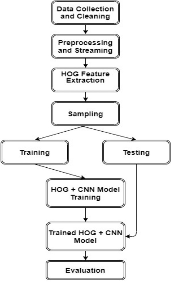
Working procedure of the proposed system

Methodology

Data Set

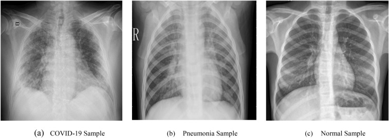
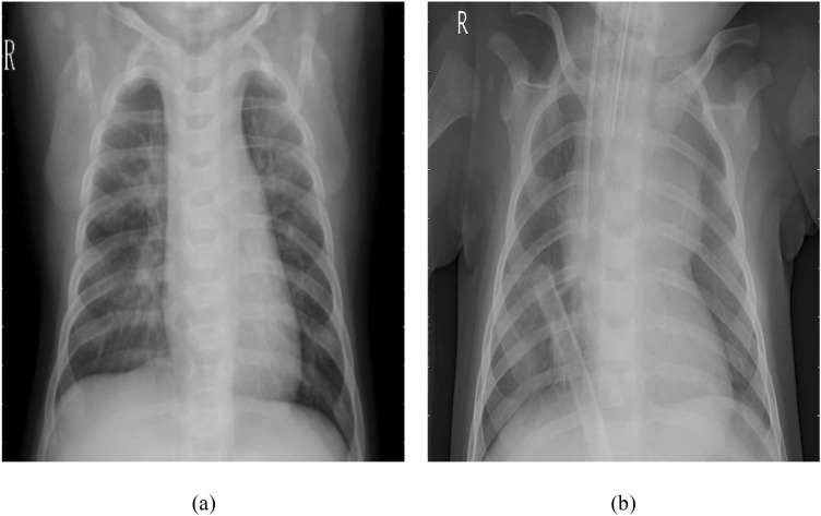
The data set is collected from Kaggle [32] that contains the posterior-anterior (PA) view of chest X-images from three categories: COVID-19, pneumonia, and normal. In Fig. 4, samples of three different categories from the data set are shown. The data set contains a total of 6432 chest X-ray images among them 576 images are from COVID-19-affected patients, 4273 images from pneumonia-affected patients, and 1583 images are from normal patients. In the preprocessing step at first, the images are converted into grayscale. Then the images are reshaped into ($64\times 128$) to match with the original HOG feature extraction algorithm. The HOG feature of each image is of the shape (1 × 3780. The generated data set contains the HOG feature of each sample X-ray image from the original data set associated with the corresponding label. The shape of the generated data set is ($6432\times 3781$). A 9:1 split was performed on the data set to generate the train and test data set. Data samples contained in the train and test data set are 5788 and 644, respectively.

Fig. 4.

PA view of the chest X-rays from the data set

HOG

A feature descriptor is an algorithm that takes an image as input and outputs a feature array or feature vector. Feature descriptors simplify an input image into numerical representation by encoding useful information in the feature vector and throwing away extraneous information. Feature descriptors can differentiate among various objects based on their various properties. Some examples of feature descriptors are: scale-invariant feature transform (SIFT), Binary Robust Independent Elementary Features (BRIEF), Features from Accelerated Segment Tree (FAST), Oriented FAST and Rotated BRIEF (ORB), Histogram of Oriented Gradients (HOG), etc.

The Histogram of Oriented Gradients (HOG) is a robust feature descriptor used widely in object detection and recognition. While the HOG features are primarily used for object detection, the extracted features can be passed to a classifier to perform object recognition as well. The main distinction between HOG and other feature descriptors, such as SIFT, shape contexts, and edge orientation histograms, is that dense uniformly spaced grids are used for the calculation of HOG and local contrast normalization is used for accuracy improvement. The HOG descriptor is geometric and photometric transformations invariant.

In HOG, the histograms of orientations of gradients are used as features. Gradients (x and y directions) are useful features that can represent complex shapes, such as edges and corners. The direction of the gradient represents the direction of change in pixel intensity in an image, whereas the magnitude represents the severity of the change. For an image $f(x,y)$, the gradient of the image can be represented as

$$\mathrm{\nabla }f=\left[\begin{array}{c}{g}_x\\ g_y\end{array}\right]=\left[\begin{array}{c}\frac{\partial f}{\partial x}\\ \frac{\partial f}{\partial y}\end{array}\right].$$

Here, $\frac{\partial f}{\partial x}$ is the derivative of the image with respect to $x$ and $\frac{\partial f}{\partial y}$ is the derivative of the image with respect to $y$. The derivatives can be further calculated as follows:

$$f_x\left(x\right)=\frac{\partial f}{\partial x}=f\left(x,+,1\right)-f\left(x,-,1\right),$$

$$f_y\left(y\right)=\frac{\partial f}{\partial y}=f\left(y,+,1\right)-f\left(y,-,1\right).$$

In practice, the derivatives are calculated by convoluting the images along the $x$- and $y$-axes using the kernels $\begin{array}{ccc}[-1& 0& 1\end{array}]$ and $\left[\begin{array}{c}-1\\ 0\\ 1\end{array}\right]$. After the gradients are calculated the magnitude and direction of the gradients can be calculated using the following formulas:

$$g=\sqrt{{g_x}^2+{g_y}^2},$$

$$\theta ={\tan }^{-1}\frac{g_y}{g_x}.$$

In cases of edges and corners (abrupt large changes in intensity), the gradient magnitude is very large. In smooth regions (no abrupt changes in intensity), the gradient magnitude is essentially zero. Thus, a lot of redundant information in the background of images is removed while calculating the gradients.

While calculating HOG, at first, patches from images are cropped and resized to ($64\times 128\times 1$). Then the resized patches are divided into ($8\times 8$) cells and the histogram of gradients along the x- and y-axes are calculated for each cell. Histograms represent the frequency of certain values. In this case, the histogram is calculated for nine angles: 0, 20, 40, 60, 80, 100, 120, 140, and 160. The gradient magnitude value is added with the value present in the corresponding gradient direction value in the histogram. The histogram is thus output as an array of size ($1\times 9$). As the histogram is calculated over a patch, the system becomes robust to noise. Since the brightness of the image is not evenly distributed some portions of the chest X-ray image are brighter compared to other portions. Therefore, after the histograms are calculated, they are normalized to reduce the system’s sensitivity to overall lighting. In general, the L2 normalization is done on ($16\times 16$) blocks. A ($16\times 16$) block with 0 overlaps contains four ($8\times 8$) histograms of gradients. The histograms are concatenated to generate an array of size ($1\times 36$). For a vector $H=\left[h,1,,,h,2,,,h,3,,,h,4,,,\cdots ,,,h_n\right]$, the L2 norm of the vector is calculated as follows:

$$H_{l2}=\left|H\right|=\sqrt{{h_1}^2+{h_1}^2+{h_1}^2+{h_1}^2},$$

$$H_{\mathrm{n}\mathrm{o}\mathrm{r}\mathrm{m}}=\frac{H}{\left|H\right|}.$$

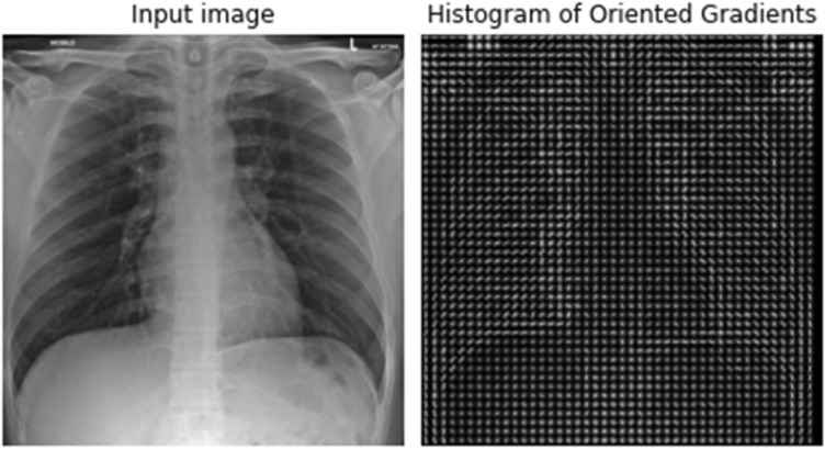
These normalized vectors are then used as features to perform various computer vision tasks. There are ($7\times 15$) or 105 blocks of ($16\times 16$) which are shown in Fig. 5. Each of these 105 blocks contains a vector of size (1 $\times 36$). Hence, the total features of the image would be $105\times 36=3780$ features. We then send these features to a convolutional neural network (CNN) for performing object recognition. Figure 6 shows a chest X-ray image from the data set and its calculated histogram of oriented gradients.

Fig. 5.

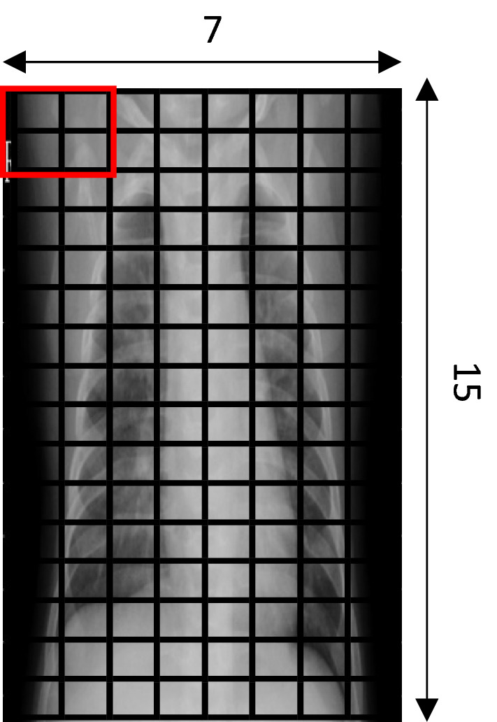
HOG feature calculation

Fig. 6.

Input image and its calculated histogram of oriented gradients

CNN

Convolutional Neural Networks (CNN or ConvNet) are deep neural networks used predominantly in computer vision tasks. CNN’s are the representation of biological processes as the connection patterns between neurons are comparable to biological visual systems. CNN’s require little to no pre-processing than traditional image classification algorithms as CNN’s learn to automatically extract features. In the field of image processing, convolution is a transformation operation, where a small matrix of numbers also known as filter or kernel is passed over an image and generally weighted average values are calculated. The mathematical formulation for convolution in 2D space is as follows:

$$y\left[i,,,j\right]=\sum _m\sum _{n}k\left[m,,,n\right]·x[i-m,j-n].$$

Here, $x$ and $k$ are the input image and the convolution kernel. The convolution operation between them results in the output image denoted by $y$. The indices $(m,n)$ and $(i,j)$ are concerned with the height and width of the kernel and the input image, respectively. As convolutions generally shrink the input image, various types of paddings are used to facilitate convolutions of the entire image. Stride is also another value that denotes the pixel amount the kernel moves after each convolution. In deep learning, images are generally resized to have equal weight and height. Kernels are also generally designed to have equal height and weight. For example, $3\times 3$, $5\times 5$, etc. are some commonly used kernel sizes.

If we consider the input image to be of the shape $\left(n_{\mathrm{i}\mathrm{n}},,,,n_{\mathrm{i}\mathrm{n}}\right)$, the shape of the kernel to be of $\left(k_{\mathrm{i}\mathrm{n}},,,,k_{\mathrm{i}\mathrm{n}}\right)$, padding $p$ and stride $s$, then the dimension of $y$ is ${(n}_{\mathrm{o}\mathrm{u}\mathrm{t}},n_{\mathrm{o}\mathrm{u}\mathrm{t}})$, where

$$n_{\mathrm{o}\mathrm{u}\mathrm{t}}=\left[\frac{n_{\mathit{in}}+2p-k_{\mathit{in}}}{s},+,1\right].$$

In color images, another dimension called the color channel is included. In 3D convolution, both the input image and the kernel have 3 channels. Thus, in that case, the output image has the shape ${(n}_{\mathrm{o}\mathrm{u}\mathrm{t}},n_{\mathrm{o}\mathrm{u}\mathrm{t}},n_c)$, where $n_c$ denotes the number of channels and $n_{\mathrm{o}\mathrm{u}\mathrm{t}}$ is calculated as above.

Figure 7 depicts a general block diagram of a CNN. The input images are first convoluted using the filters to get the feature vector. Pooling layers reduce the dimensionality of the feature vector. The fully connected layers contain the neurons that learn the features. Finally, an activation function generates the prediction. While training a CNN, the error is calculated from the output. The error is then used to fine-tune the trainable parameters, i.e., the filter values and the weights of the neurons.

Fig. 7.

General CNN block diagram

HOG + CNN Model

We used a combination of HOG feature extractor and a CNN to classify among the three classes in the data set: COVID-19, pneumonia, and normal. The model consists of two modules: the HOG feature extractor module and a CNN module. Images are input to the HOG feature extractor module and for each image, a feature vector of size ($1\times 3780$) is generated. The feature vector is then reshaped to a 2D matrix of size ($60\times 63$). This feature vector is then sent to the CNN, as illustrated in Fig. 8 for proper classification. Inputs are passed through two pairs of convolution and MaxPooling layers.

Fig. 8.

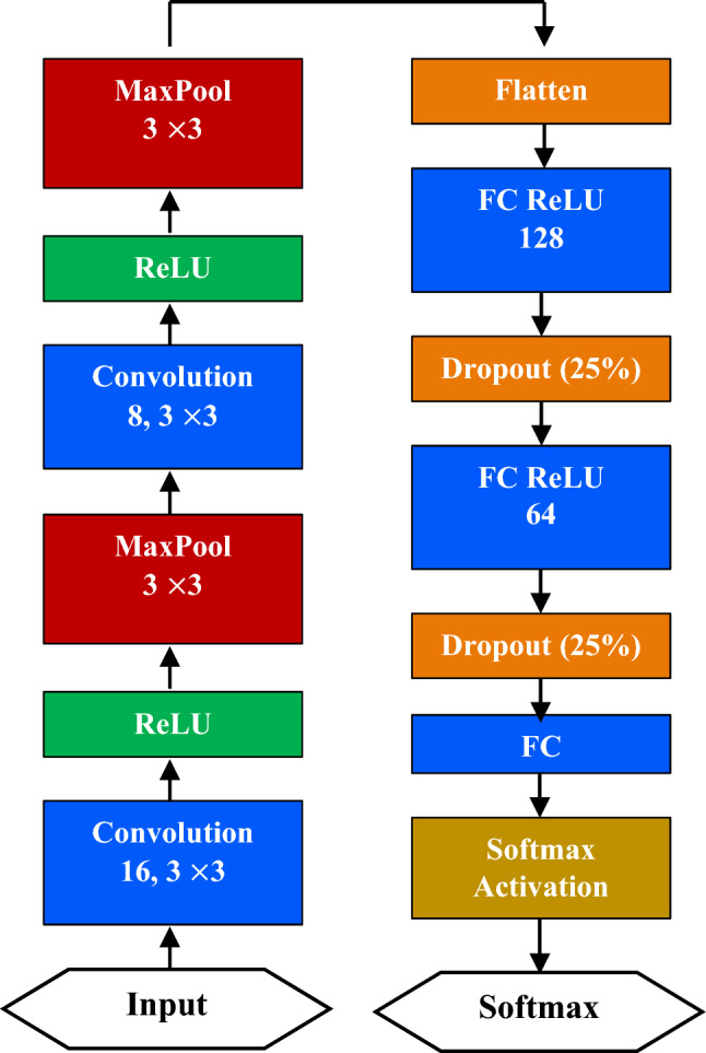
Proposed HOG + CNN model architecture

Then, a Flatten layer generates a one-dimensional weight vector from the multi-dimensional weights. Two hidden Fully Connected (FC) layers with Rectified Linear Unit (ReLU) activation each followed by a 25% Dropout layer learns the input features. Finally, an FC layer with Softmax activation classifies the input. While compiling the model, Adam is used as the optimizer and Categorical Crossentropy is used as the loss function. Several early stopping methods monitoring the validation loss and training loss are used as safeguards against model overfitting. CNN extract features from images using these convolutions. Pooling techniques, such as maximum pooling, global average pooling, etc., are used to reduce the dimensionality of the feature vector. The learning or training procedure consists of two stages:

1. Forward propagation and

2. Backward propagation.

Forward Propagation: In forward propagation, the outputs of the convolutions are first flattened to get the feature vector. Then, two transformations: A linear transformation and a non-linear transformation are performed on the data. The linear transformation can be represented as follows:

$$z=W^T.X+b.$$

Here, $W$ represents the weight matrix and $b$ represents the bias constant. $X$ is the feature vector. The shape of $W$ depends on the number of features in the feature vector and the number of neurons in the hidden label. If $l$ represents the length of the feature vector and $n$ represents the number of neurons in the layer, then $W$ has a shape of $\left(l,,,n\right).$ The output of the linear transformation is a singular integer value.

The non-linear transformation is performed by an activation function. For classification, the ReLU activation function is used. Given an input $x$, the output of the sigmoid function is as follows:

$$R\left(z\right)=\max \left(0,,,z\right).$$

Figure 9 depicts the output of the ReLU activation function. In general, any input value greater than the threshold value is output as 1, and 0 otherwise. In the forward propagation stage, the values of the filters, as well as the weights and bias are randomly initialized. Then the output of the model is calculated, as shown in Fig. 10. In the backward propagation stage proper values for filters, weights, and bias are learned.

Fig. 9.

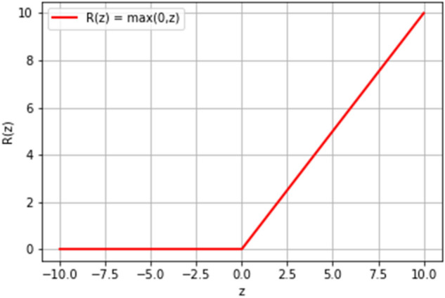
Rectified Linear Unit (ReLU) activation function for classification

Fig. 10.

Forward propagation process in a multi-class classifier

Backward Propagation: In the backward propagation stage, the error is calculated and loss is minimized using the gradient descent algorithm. The trainable values are generally updated using the following formula:

$$w^{\prime }=w\pm \eta .\mathrm{\nabla }w.$$

Here, $w$ is the learnable parameter. $w^{\prime }$ is the updated value, $w$ is the initial value, $\eta$ is the learning rate, and $\mathrm{\nabla }w$ is the gradient of the parameter.

To update the convolution kernel values, the gradient is calculated using the following formula:

$$\frac{\partial E}{\partial k}=\left(\frac{\partial E}{\partial O},·,\frac{\partial O}{\partial Z2},·,\frac{\partial Z2}{\partial A1},·,\frac{\partial A1}{\partial Z1}\right)\ast \frac{\partial Z1}{\partial k}.$$

Here, E stands for Error which is the difference between the output of the model and actual value and k is the convolution kernel. There are various ways to calculate this error. In general, the error is calculating by subtracting the prediction value from the original output value. Mean Squared Error (MSE), Mean Absolute Percentage Error (MAPE), etc. are also some of the used error calculation methods. Figure 11 represents a short overview of the computation graph of the backpropagation process in the case of a multi-class classifier. $\frac{\partial E}{\partial k}$ implies that how much the kernel values contribute to the error. Based on this value the kernel values are updated. This process is applied to all the layers to learn each layer’s learnable parameters.

Fig. 11.

Backward propagation process in a multi-class classifier

Result Analysis

The training process of the proposed model was continued for 100 epochs to escape overfitting. To optimize the loss function ADAM optimizer is used. ReLU is used as the activation function of all the layers except the output layer. The output layer uses an activation function. L2 regularizer with regularization factor 0.01 is used to develop the generalization capability of the model. Figures 12 and 13 show the accuracy and loss, respectively, in the training and testing phase.

Fig. 12.

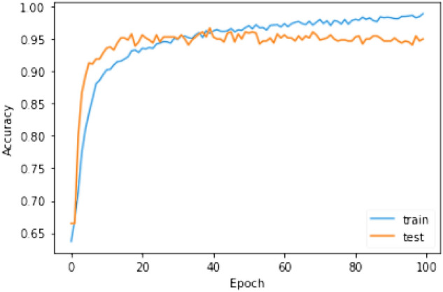
Accuracy of the model in the training and testing phase

Fig. 13.

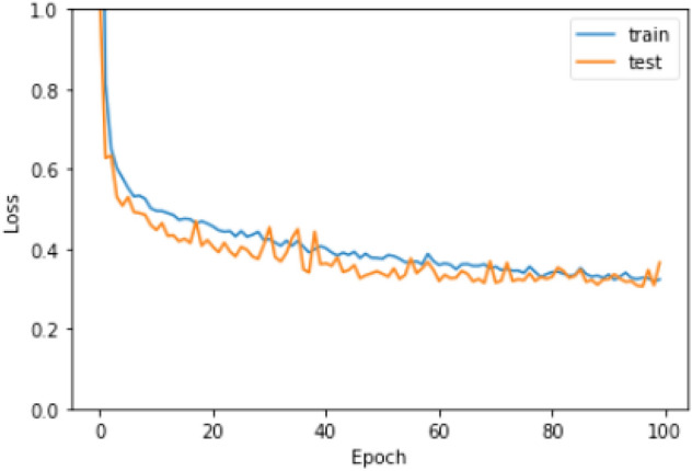
Loss of the model in the training and testing phase

Different matrices are used to evaluate the performance of a classification model. Accuracy, precision, recall, and F1-score are calculated for reporting the performance of the proposed model. Accuracy is the ratio of all the correctly predicted data points and all of the data points. The accuracy of a system denotes the total number of correctly predicted tests. The accuracy of a system helps us understand how often the system correctly classifies a data input. True Positive (TP) and True Negative (TN) are data points that the system has correctly predicted as true or false. On the other hand, False Positive (FP) and False Negative (FN) are data points that the system has incorrectly identified as true or false. For example, if the system incorrectly identified a negative data point as positive, it is calculated as FP. Similarly, if the system incorrectly identified a positive data point as negative, it is calculated as FN. Accuracy is calculated using the following formula:

$$\mathrm{A}\mathrm{c}\mathrm{c}\mathrm{u}\mathrm{r}\mathrm{a}\mathrm{c}\mathrm{y}=\frac{\mathrm{T}\mathrm{P}+\mathrm{T}\mathrm{N}}{\mathrm{T}\mathrm{P}+\mathrm{T}\mathrm{N}+\mathrm{F}\mathrm{P}+\mathrm{F}\mathrm{N}}.$$

Precision or positive predictive value represents the total number of correctly identified positive data points among all predicted positive data points. Precision can be interpreted as the calculation of accuracy for the minority class. The precision of a system is calculated using the following formula:

$$\mathrm{P}\mathrm{r}\mathrm{e}\mathrm{c}\mathrm{i}\mathrm{s}\mathrm{i}\mathrm{o}\mathrm{n}=\frac{\mathrm{T}\mathrm{P}}{\mathrm{T}\mathrm{P}+\mathrm{F}\mathrm{P}}.$$

Sensitivity is also known as true positive rate or recall is the fraction of correctly identified positive data points among all the positive data points in the data set. The recall is calculated using the following formula:

$$\mathrm{R}\mathrm{e}\mathrm{c}\mathrm{a}\mathrm{l}\mathrm{l}=\frac{\mathrm{T}\mathrm{P}}{\mathrm{T}\mathrm{P}+\mathrm{F}\mathrm{N}}.$$

F1-Score is represented as the harmonic mean of precision and recall. F1 score always resides in the range [0,1]. F1 score is calculated using the following formula:

$$F1=2\times \frac{\mathrm{P}\mathrm{r}\mathrm{e}\mathrm{c}\mathrm{i}\mathrm{s}\mathrm{i}\mathrm{o}\mathrm{n}\times \mathrm{R}\mathrm{e}\mathrm{c}\mathrm{a}\mathrm{l}\mathrm{l}}{\mathrm{P}\mathrm{r}\mathrm{e}\mathrm{c}\mathrm{i}\mathrm{s}\mathrm{i}\mathrm{o}\mathrm{n}+\mathrm{R}\mathrm{e}\mathrm{c}\mathrm{a}\mathrm{l}\mathrm{l}}.$$

As precision and recall are inversely related, meaning increasing precision results in decreasing recall and vice versa, the F1 score is a better representation of model performance.

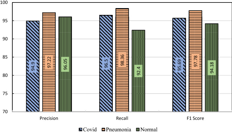
In Fig. 14, the confusion matrix of the proposed model is presented which is highly used for visualizing the performance of a classification model. The rows of the matrix represent actual classes and the columns represent the predicted classes. The precision, recall, and F1 score are presented in Fig. 15 on a per-class basis, meaning the multiclass confusion matrix was transformed into one-vs-all for every individual class and the appropriate performance matrices were calculated. The overall accuracy of the system is found 96.74%.

Fig. 14.

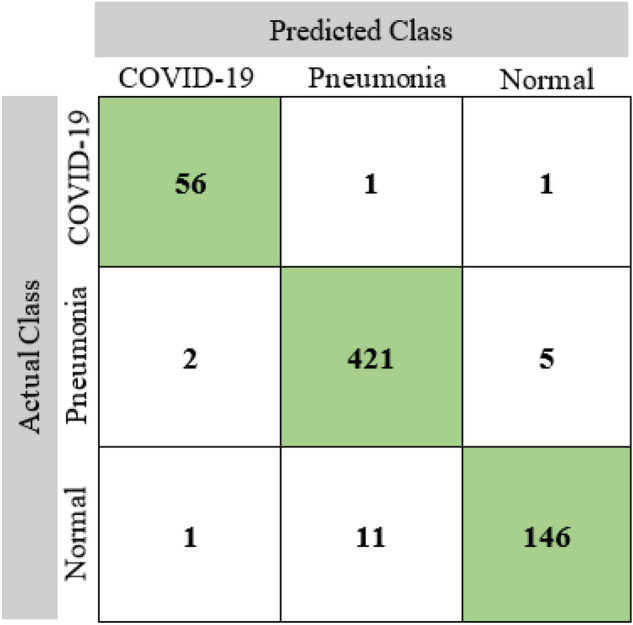
Confusion matrix of the proposed model

Fig. 15.

Graphical representation of the performance of the HOG + CNN model

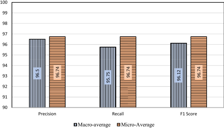
We also evaluated the performance of the proposed model using the Micro-average and Macro-average method to properly demonstrate the capability of the system. Precision and Recall in the Micro-average method in a 3-class scenario are calculated using the following formulas:

$${\mathrm{P}\mathrm{r}\mathrm{e}\mathrm{c}\mathrm{i}\mathrm{s}\mathrm{i}\mathrm{o}\mathrm{n}}_{\mathrm{m}\mathrm{i}\mathrm{c}\mathrm{r}\mathrm{o}}=\frac{{\mathrm{T}\mathrm{P}}_1+{\mathrm{T}\mathrm{P}}_2+{\mathrm{T}\mathrm{P}}_3}{{\mathrm{T}\mathrm{P}}_1+{\mathrm{T}\mathrm{P}}_2+{\mathrm{T}\mathrm{P}}_3+{\mathrm{F}\mathrm{P}}_1+{\mathrm{F}\mathrm{P}}_2+{\mathrm{F}\mathrm{P}}_3},$$

$${\mathrm{R}\mathrm{e}\mathrm{c}\mathrm{a}\mathrm{l}\mathrm{l}}_{\mathrm{m}\mathrm{i}\mathrm{c}\mathrm{r}\mathrm{o}}=\frac{{\mathrm{T}\mathrm{P}}_1+{\mathrm{T}\mathrm{P}}_2+{\mathrm{T}\mathrm{P}}_3}{{\mathrm{T}\mathrm{P}}_1+{\mathrm{T}\mathrm{P}}_2+{\mathrm{T}\mathrm{P}}_3+{\mathrm{F}\mathrm{N}}_1+{\mathrm{F}\mathrm{N}}_2+{\mathrm{F}\mathrm{N}}_3}.$$

Precision and Recall in Macro-average in a 3-class scenario method are calculated using the following formulas:

$${\mathrm{P}\mathrm{r}\mathrm{e}\mathrm{c}\mathrm{i}\mathrm{s}\mathrm{i}\mathrm{o}\mathrm{n}}_{\mathrm{m}\mathrm{a}\mathrm{c}\mathrm{r}\mathrm{o}}=\frac{{\mathrm{P}\mathrm{r}\mathrm{e}\mathrm{c}}_1+{\mathrm{P}\mathrm{r}\mathrm{e}\mathrm{c}}_2+{\mathrm{P}\mathrm{r}\mathrm{e}\mathrm{c}}_3}{3},$$

$${\mathrm{R}\mathrm{e}\mathrm{c}\mathrm{a}\mathrm{l}\mathrm{l}}_{\mathrm{m}\mathrm{a}\mathrm{c}\mathrm{r}\mathrm{o}}=\frac{{\mathrm{R}\mathrm{e}\mathrm{c}\mathrm{a}\mathrm{l}\mathrm{l}}_1+{\mathrm{R}\mathrm{e}\mathrm{c}\mathrm{a}\mathrm{l}\mathrm{l}}_2+{\mathrm{R}\mathrm{e}\mathrm{c}\mathrm{a}\mathrm{l}\mathrm{l}}_3}{3}.$$

In both cases, the F1 score is calculated based on precision and recall. Micro-average and Macro-average of the matrices precision, recall, and F1-score are calculated and graphically presented in Fig. 16.

Fig. 16.

Graphical representation of Micro-average and Macro-average of performance of the HOG + CNN model

Figure 17 shows the Receiver Operating Characteristic (ROC) curve and Area Under the Curve (AUC) of the proposed HOG + CNN model. ROC is a graphical plot that shows a binary classifier system's diagnostic potential as its threshold of discrimination is varied. The percentage of the region under this ROC curve is AUC, varying from 0 to 1. AUC is a single number that summarizes the output of a classifier by evaluating the ranking about the division of the classes. ROC curve is generated by plotting False Positive Rate (FPR) along the x-axis and True Positive Rate (TPR) along the y-axis. FPR and TPR are calculated using the following formulas:

$$\mathrm{T}\mathrm{r}\mathrm{u}\mathrm{e}\mathrm{P}\mathrm{o}\mathrm{s}\mathrm{i}\mathrm{t}\mathrm{i}\mathrm{v}\mathrm{e}\mathrm{R}\mathrm{a}\mathrm{t}\mathrm{e}=\frac{\mathrm{T}\mathrm{r}\mathrm{u}\mathrm{e}\mathrm{P}\mathrm{o}\mathrm{s}\mathrm{i}\mathrm{t}\mathrm{i}\mathrm{v}\mathrm{e}}{\mathrm{T}\mathrm{r}\mathrm{u}\mathrm{e}\mathrm{P}\mathrm{o}\mathrm{s}\mathrm{i}\mathrm{t}\mathrm{i}\mathrm{v}\mathrm{e}+\mathrm{F}\mathrm{a}\mathrm{l}\mathrm{s}\mathrm{e}\mathrm{N}\mathrm{e}\mathrm{g}\mathrm{a}\mathrm{t}\mathrm{i}\mathrm{v}\mathrm{e}},$$

$$\mathrm{F}\mathrm{a}\mathrm{l}\mathrm{s}\mathrm{e}\mathrm{P}\mathrm{o}\mathrm{s}\mathrm{i}\mathrm{t}\mathrm{i}\mathrm{v}\mathrm{e}\mathrm{R}\mathrm{a}\mathrm{t}\mathrm{e}=\frac{\mathrm{F}\mathrm{a}\mathrm{l}\mathrm{s}\mathrm{e}\mathrm{P}\mathrm{o}\mathrm{s}\mathrm{i}\mathrm{t}\mathrm{i}\mathrm{v}\mathrm{e}}{\mathrm{T}\mathrm{r}\mathrm{u}\mathrm{e}\mathrm{N}\mathrm{e}\mathrm{g}\mathrm{a}\mathrm{t}\mathrm{i}\mathrm{v}\mathrm{e}+\mathrm{F}\mathrm{a}\mathrm{l}\mathrm{s}\mathrm{e}\mathrm{P}\mathrm{o}\mathrm{s}\mathrm{i}\mathrm{t}\mathrm{i}\mathrm{v}\mathrm{e}}.$$

Fig. 17.

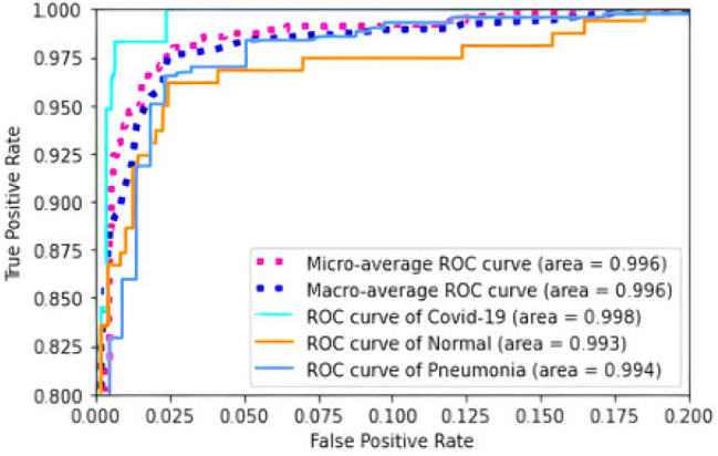
ROC curve and AUC for the HOG + CNN model

The proposed HOG + CNN model is a classifier with three different classes. To generate the ROC curve one-vs-all approach is used. For example, when plotting the ROC curve of class COVID-19, the other two classes fall into the NOT-COVID-19 class. In this way, the ROC curve for pneumonia and normal classes is generated. In Fig. 17, micro-average and macro-average of the ROC curves for three different classes are also shown. The area under the Micro-average and Macro-average ROC curves is 0.996 in both cases. AUC of ROC curves of COVID-19, pneumonia, and normal classes in the one-vs-all approach are, respectively, 0.998, 0.994, and 0.993.

In Table 1, the performance of some related classification techniques using chest X-ray (CXR) images is compared with our proposed model in terms of accuracy. The models compared hare all used CXR images of classification but the number of images in different classes in the data set varies. Here, the proposed method outstands among all the compared models by performance. From the table, it is found that [20, 24], and [29] have accuracy below 90% and [21], and [26] have accuracy very close to the proposed model.

Table 1.

Comparison of the proposed HOG + CNN model with related works using chest X-ray images

Author	Architecture	CXR Images/class	Accuracy %
Razzak et al. [20]	MobileNet	COVID-19 (200) Viral pneumonia (200) Bacterial pneumonia (200) Normal (200)	80.95
Asif and Wenhui [21]	Inception V3	COVID-19 (864) Pneumonia (1345) Normal (1341)	96
Pathari and Rahul [22]	MobileNet V3	COVID-19 (6000) Pneumonia (6000) Normal (6000)	95.58
Makris et al. [23]	VGG16	COVID-19 (112) Pneumonia (112) Normal (112)	95.88
Gomes et al. [24]	SVM	COVID-19 (464) Viral pneumonia (1490) Bacterial pneumonia (2783) Normal (1583)	89.78
Elaziz et al. [26]	K Nearest Neighbor (KNN)	COVID-19 (216) Normal (1675)	96.09
Wang and A. Wong [27]	Deep Convolutional Neural Network (COVID-Net)	COVID-19 (358) Pneumonia (5538) Normal (8066)	93.3
Duran-Lopez et al. [28]	Deep Convolutional Neural Network (COVID-XNet)	COVID-19 (2589) Normal (4337)	94.43
Oh et al. [29]	ResNet-18	Viral Pneumonia + COVID-19 (200) Bacterial pneumonia (54) Tuberculosis (57) Normal (191)	88.9
Proposed HOG + CNN Model	Deep Convolutional Neural Network (HOG + CNN)	COVID-19 (576) Pneumonia (4273) Normal (1583)	96.74

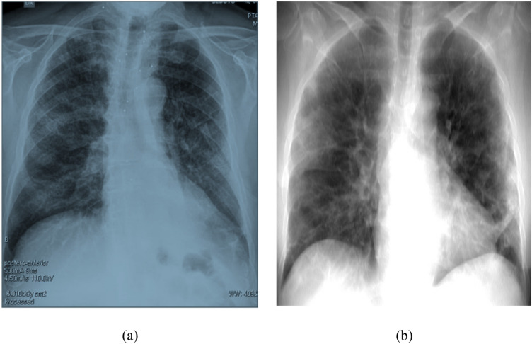
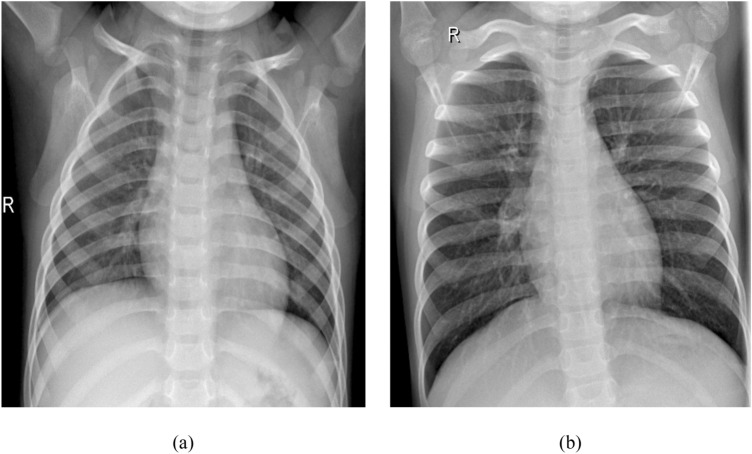
Although the proposed system has very good performance in detecting COVID-19-related pneumonia from chest X-ray images, some images are still misclassified in some cases. Figure 18 shows some misclassification samples, where actual COVID-19 positive pneumonia was misclassified. In Fig. 19, actual pneumonia cases were misclassified into healthy and COVID-19-related pneumonia. Figure 20 shows normal cases being misclassified as various forms of pneumonia.

Fig. 18.

Actual COVID positive but predicted; a normal, b pneumonia

Fig. 19.

Actual pneumonia positive but predicted; a normal, b COVID

Fig. 20.

Actual normal positive but predicted; a pneumonia, b COVID

Conclusion

The current coronavirus pandemic requires effective collaboration from all walks of life for proper containment and cure. Recognizing COVID-19 infected patients is the first step towards curbing the exponential infection rate of the coronavirus. In this paper, we have presented a novel HOG + CNN-based model for identifying COVID-19 infected patients using chest X-ray images. The model is highly capable of diagnosing COVID-19 infections in chest X-ray images. In the future, the effects of using other feature extraction methods combined with CNNs can be observed. The performance of these models can still be improved using larger data sets. Thus, the amount of COVID-19 infected chest X-ray data is a severe limitation. Although chest X-ray-based methods show very promising performance in recognizing COVID-19 infected patients from chest X-ray images, they are still not as accurate as the time-consuming PCR-based methods. However, these methods can be used as initial screening methods to select patients for the PCR test.

Declarations

Conflict of Interest

The authors declare no conflicts of interest.

References

- 1.WHO | World Health Organization. https://www.who.int/. Accessed Aug 18, 2020.
- 2.What Is Coronavirus? | Johns Hopkins Medicine. https://www.hopkinsmedicine.org/health/conditions-and-diseases/coronavirus. Accessed Aug 18, 2020.
- 3.Coronavirus Map: Tracking the Global Outbreak - The New York Times. https://www.nytimes.com/interactive/2020/world/coronavirus-maps.html. Accessed Aug 18, 2020.
- 4.WHO Director-General’s opening remarks at the media briefing on COVID-19—11 March 2020. https://www.who.int/dg/speeches/detail/who-director-general-s-opening-remarks-at-the-media-briefing-on-covid-19---11-march-2020. Accessed Aug 18, 2020.
- 5.Symptoms of Coronavirus | CDC. https://www.cdc.gov/coronavirus/2019-ncov/symptoms-testing/symptoms.html. Accessed Aug 18, 2020.
- 6.Haleem A, Javaid M, Vaishya R. Effects of COVID-19 pandemic in daily life. Curr Med Res Pract. 2020;10(2):78–79. doi: 10.1016/j.cmrp.2020.03.011. [DOI] [PMC free article] [PubMed] [Google Scholar]
- 7.Testing for COVID-19 | CDC. https://www.cdc.gov/coronavirus/2019-ncov/symptoms-testing/testing.html. Accessed Aug 18, 2020.
- 8.Loeffelholz MJ, Tang YW. Laboratory diagnosis of emerging human coronavirus infections–the state of the art. Emerg Microbes Infect. 2020;9(1):747–756. doi: 10.1080/22221751.2020.1745095. [DOI] [PMC free article] [PubMed] [Google Scholar]
- 9.Long C, et al. Diagnosis of the Coronavirus disease (COVID-19): rRT-PCR or CT? Eur J Radiol. 2020;126:108961. doi: 10.1016/j.ejrad.2020.108961. [DOI] [PMC free article] [PubMed] [Google Scholar]
- 10.Rubin GD, et al. The role of chest imaging in patient management during the COVID-19 pandemic: a multinational consensus statement from the Fleischner society. Radiology. 2020;296(1):172–180. doi: 10.1148/radiol.2020201365. [DOI] [PMC free article] [PubMed] [Google Scholar]
- 11.Ai T, et al. Correlation of chest CT and RT-PCR testing for coronavirus disease 2019 (COVID-19) in China: a report of 1014 cases. Radiology. 2020;296(2):E32–E40. doi: 10.1148/radiol.2020200642. [DOI] [PMC free article] [PubMed] [Google Scholar]
- 12.Li Y, et al. Stability issues of RT-PCR testing of SARS-CoV-2 for hospitalized patients clinically diagnosed with COVID-19. J Med Virol. 2020;92(7):903–908. doi: 10.1002/jmv.25786. [DOI] [PMC free article] [PubMed] [Google Scholar]
- 13.Test for Current Infection | CDC. https://www.cdc.gov/coronavirus/2019-ncov/testing/diagnostic-testing.html. Accessed Aug 18, 2020.
- 14.Pesapane F, Codari M, Sardanelli F. Artificial intelligence in medical imaging: threat or opportunity? Radiologists again at the forefront of innovation in medicine. Eur Radiol Exp. 2018 doi: 10.1186/s41747-018-0061-6. [DOI] [PMC free article] [PubMed] [Google Scholar]
- 15.Wang W, et al. Medical image classification using deep learning. In: Intelligent systems reference library. Berlin: Springer; 2020. pp. 33–51. [Google Scholar]
- 16.Li X, Zhang R, Wang Q, Zhang H. Autoencoder constrained clustering with adaptive neighbors. IEEE Trans Neural Networks Learn Syst. 2021;32(1):443–449. doi: 10.1109/TNNLS.2020.2978389. [DOI] [PubMed] [Google Scholar]
- 17.Salehi S, Abedi A, Balakrishnan S, Gholamrezanezhad A. Coronavirus disease 2019 (COVID-19): a systematic review of imaging findings in 919 patients. Am J Roentgenol. 2020;215(1):87–93. doi: 10.2214/AJR.20.23034. [DOI] [PubMed] [Google Scholar]
- 18.Tapé C, Byrd KM, Aung S, Lonks JR, Flanigan TP, and Rybak NR. COVID-19 in a patient presenting with syncope and a normal chest x-ray. R I Med J 2013. 2020;103(3):50–51. Available: http://www.ncbi.nlm.nih.gov/pubmed/32226962. Accessed: Mar 23, 2021. [PMC free article] [PubMed]
- 19.Zhao D, et al. A comparative study on the clinical features of coronavirus 2019 (COVID-19) pneumonia with other pneumonias. Clin Infect Dis. 2020;71(15):756–761. doi: 10.1093/cid/ciaa247. [DOI] [PMC free article] [PubMed] [Google Scholar]
- 20.Razzak I, Naz S, Rehman A, Khan A, Zaib A. Improving coronavirus (COVID-19) diagnosis using deep transfer learning. medRxiv. 2020 doi: 10.1101/2020.04.11.20054643. [DOI] [Google Scholar]
- 21.Asif S, Wenhui Y. Automatic detection of COVID-19 using x-ray images with deep convolutional neural networks and machine learning. Cold Spring Harbor Lab Press. 2020 doi: 10.1101/2020.05.01.20088211. [DOI] [Google Scholar]
- 22.Pathari S, Rahul U. Automatic detection of COVID-19 and pneumonia from chest x-ray using transfer learning. medRxiv. 2020 doi: 10.1101/2020.05.27.20100297. [DOI] [Google Scholar]
- 23.Makris A, Kontopoulos I, Tserpes K. COVID-19 detection from chest x-ray images using Deep Learning and Convolutional Neural Networks. medRxiv. 2020 doi: 10.1101/2020.05.22.20110817. [DOI] [Google Scholar]
- 24.Gomes JC, et al. IKONOS: an intelligent tool to support diagnosis of COVID-19 by texture analysis of x-ray images. medRxiv. 2020 doi: 10.1101/2020.05.05.20092346. [DOI] [Google Scholar]
- 25.Khuzani AZ, Heidari M, Shariati SA. COVID-Classifier: an automated machine learning model to assist in the diagnosis of COVID-19 infection in chest x-ray images. medRxiv Prepr Serv Health Sci. 2020 doi: 10.1101/2020.05.09.20096560. [DOI] [PMC free article] [PubMed] [Google Scholar]
- 26.Elaziz MA, et al. New machine learning method for imagebased diagnosis of COVID-19. PLoS ONE. 2020 doi: 10.1371/journal.pone.0235187. [DOI] [PMC free article] [PubMed] [Google Scholar]
- 27.Wang L, Wong A. COVID-Net: a tailored deep convolutional neural network design for detection of COVID-19 cases from chest x-ray images. 2020. http://arxiv.org/abs/2003.09871. Accessed: Aug 23, 2020. [DOI] [PMC free article] [PubMed]
- 28.Duran-Lopez L, Dominguez-Morales JP, Corral-Jaime J, Vicente-Diaz S, Linares-Barranco A. COVID-XNet: a custom deep learning system to diagnose and locate COVID-19 in chest x-ray images. Appl Sci. 2020;10(16):5683. doi: 10.3390/app10165683. [DOI] [Google Scholar]
- 29.Oh Y, Park S, Ye JC. Deep learning COVID-19 features on CXR using limited training data sets. IEEE Trans Med Imaging. 2020;39(8):2688–2700. doi: 10.1109/TMI.2020.2993291. [DOI] [PubMed] [Google Scholar]
- 30.Shah V, Keniya R, Shridharani A, Punjabi M, Shah J, Mehendale N. Diagnosis of COVID-19 using CT scan images and deep learning techniques. medRxiv. 2020 doi: 10.1101/2020.07.11.20151332. [DOI] [PMC free article] [PubMed] [Google Scholar]
- 31.Ko H, et al. COVID-19 pneumonia diagnosis using a simple 2d deep learning framework with a single chest CT image: model development and validation. J Med Internet Res. 2020;22(6):e19569. doi: 10.2196/19569. [DOI] [PMC free article] [PubMed] [Google Scholar]
- 32.Chest X-ray (COVID-19 & Pneumonia) | Kaggle. https://www.kaggle.com/prashant268/chest-xray-covid19-pneumonia. Accessed Oct 02, 2020.