

Abstract

Blending hydrogen into the natural gas pipeline is considered as a feasible way for large-scale and long-distance delivery of hydrogen. However, the blended hydrogen can exert major impacts on the Joule–Thomson (J–T) coefficient of natural gas, which is a significant parameter for liquefaction of natural gas and formation of natural gas hydrate in engineering. In this study, the J–T coefficient of natural gas at different hydrogen blending ratios is numerically investigated. First, the theoretical formulas for calculating the J–T coefficient of the natural gas–hydrogen mixture using the Soave–Redlich–Kwong (SRK) equation of state (EOS), Peng–Robinson EOS (PR-EOS), and Benedict–Webb–Rubin–Starling EOS (BWRS-EOS) are, respectively, derived, and the calculation accuracy is verified by experimental data. Then, the J–T coefficients of natural gas at six different hydrogen blending ratios and thermodynamic conditions are calculated and analyzed using the derived theoretical formulas and a widely used empirical formula. Results indicate that the J–T coefficient of the natural gas–hydrogen mixture decreases approximately linearly with the increase of the hydrogen blending ratio. When the hydrogen blending ratio reaches 30% (mole fraction), the J–T coefficient of the natural gas–hydrogen mixture decreases by 40–50% compared with that of natural gas. This work also provides a J–T coefficient database of a methane–hydrogen mixture with a hydrogen blending ratio of 5–30% at a pressure of 0.5–20 MPa and temperatures of 275, 300, and 350 K as a reference and a benchmark for interested readers.
1. Introduction
With the increasingly serious global warming and the depletion of traditional fossil fuels, clean renewable energy has attracted considerable attention in recent years.1 However, due to the uneven distribution of renewable resources, system-wide oversupply, and other reasons, renewable energy has not been fully utilized and consumed. The waste of surplus renewable energy generation is commonly seen in many countries. As a kind of clean energy carrier, hydrogen has the advantages of wide sources and zero-carbon emission. It can be produced from renewable energies such as wind energy, nuclear energy, electric energy, etc. Through the power-to-gas (P2G) technology, surplus renewable energy generation can be converted to gaseous hydrogen; thus, it is viewed as an effective way to solve the wastage of renewable energy generation.2−5 The research of P2G technology can date back to earlier years in countries such as Germany and the United States. For example, in Europe alone there are more than 45 P2G projects in operation and under construction. Between hydrogen generation by P2G projects and hydrogen consumption by users, hydrogen delivery is a key link. For larger economic benefits and shorter transportation periods, blending hydrogen into natural gas is considered as one of the best feasible ways to achieve large-scale, long-distance transport of hydrogen using existing natural gas pipelines or pipe networks.6
For gas transportation, consideration must be given to the Joule–Thomson (J–T) effect (also known as the throttling effect). The J–T effect was first observed in an experiment conducted by James Prescott Joule and William Thomson in 1852 and is a thermodynamic process that occurs when a fluid expands from high pressure to low pressure at constant enthalpy.7 If the J–T coefficient is positive, then the fluid cools upon expansion, and if it is negative, the fluid warms upon expansion. The cooling produced in J–T expansion has been a double-edged sword in natural gas engineering. For example, the temperature drop caused by the J–T effect during natural gas transportation can cause gas hydrate blockage at the pipeline valves;8,9 in the production of natural gas hydrate, the temperature change induced by the J–T effect has significant impacts on the production efficiency;10 in natural gas liquefaction, the cooling produced in the J–T expansion can be used to liquefy natural gas,11 etc. Therefore, it is of great engineering significance to study the J–T effect of natural gas. Compared with traditional natural gas without hydrogen, the composition and relative content of natural gas are changed upon hydrogen blending, resulting in variations in its physical and thermodynamic properties. Thus, for the natural gas–hydrogen mixture, hydrogen blending can exert great influences on the J–T effect. Accurately calculating the J–T coefficient of the natural gas–hydrogen mixture and revealing the influences of hydrogen blending on the J–T effect are of great importance. At present, the widely used methods for predicting the J–T coefficient include experimental measurement,12−16 pressure–enthalpy chart,7 empirical formula,7 molecular simulation,17−19 theoretical calculation using equation of state (EOS),20−24 etc.
In the aspect of experimental measurements, many scholars measured the J–T coefficient of different gases via experiments. The basic experimental principle of J–T expansion can be summarized as follows: a gas with volume V1, pressure p1, and temperature T1 flows through a porous membrane, pushed by a piston at pressure p1; the gas expands against a piston at a lower pressure p2 until all of the gas has been transferred to the other side of the membrane with a final volume V2 and temperature T2, and then the J–T coefficient can be calculated by the pressure and temperature changes before and after expansion. From the 1970s to the 1990s, Francis et al.12−14 designed flow calorimeters to measure the specific heat capacity and the J–T coefficient. The J–T coefficients of ethanol, benzene, and cyclohexane vapors at different temperatures and pressures were measured in their study. Cuscó et al.15 applied an improved flow calorimeter to measure the J–T coefficients of N2 and CO2 at high temperature and high pressure. Ernst et al.16 measured the J–T coefficients of CH4, CH4–C2H6 mixture, and natural gas at different conditions, and the experimental results provide an important reference and contribute to the experimental basis for the formulation of an EOS.
In terms of numerical calculation, current calculation methods for the J–T coefficient mainly include the pressure–enthalpy chart,7 empirical formula,7 molecular simulation,17−19 and theoretical calculation using EOS.20−24 When the temperature and pressure before expansion and the pressure after expansion are known, the temperature after expansion can be obtained by reading the pressure–enthalpy chart, and the J–T coefficient can be calculated.7 This pressure–enthalpy chart is simple to read and is commonly used in engineering practice. However, it is worth noting that this method is not a general approach because the pressure–enthalpy chart is usually plotted for a specific natural gas mixture. Compared with the pressure–enthalpy chart, the empirical formula for calculating the J–T coefficient of natural gas is a general method with wide application scopes.7 When the specific heat capacity, the reduced temperature and pressure, and the critical temperature and pressure of natural gas are known, the J–T coefficient can be calculated using the empirical formula. However, the calculation accuracy of the empirical formula is relatively low. For the mechanism study, molecular simulation is a valuable tool for investigating the J–T effect from a microscopic point of view. For example, Vrabec et al.17 applied molecular simulation and four equations of state to calculate the J–T coefficients of six different natural gas mixtures. It was found that the molecular simulation is competitive with state-of-the-art EOS in predicting J–T inversion curves. Figueroa-Gerstenmaier et al.18 carried out molecular simulations on the J–T coefficient of various refrigerants over a wide range of thermodynamic conditions, and the simulation results were compared with pseudo-experimental-results obtained from the REFPROP software package. Zhang et al.19 analyzed the throttling mechanism of CO2 at different states from a molecular perspective, and a method for predicting the J–T coefficient of pipeline CO2 was put forward using the multivariate nonlinear regression method. It is worth pointing out that although molecular simulation can reveal the mechanism of the J–T effect and calculate the J–T coefficient from a microcosmic perspective, the application of this method is always limited by the high computational costs. In addition, the molecular simulation system is usually simplified and it cannot fully reproduce the real physical system of natural gas.
For theoretical calculation of the J–T coefficient using the EOS, the accuracy depends on the selected EOS, and there have been extensive related studies. Tay et al.20 applied the population balance model to simulate the condensation process of nonequilibrium water, and the influence of the J–T effect on the dehydration process of natural gas was analyzed using SRK-EOS. Haghighi et al.21 compared the performance of five EOSs to predict the J–T inversion curve. Results illustrated that the selected EOSs can well predict the low-temperature branch of the J–T inversion curve, except for the Mohsennia–Modarres–Mansoori EOS. In addition, the high-temperature branch and peak value of the inversion curve turned out to be sensitive to the adopted EOS. Abbas et al.22 calculated the J–T coefficients of CO2, Ar, CO2–Ar mixture, and CH4–C2H6 mixture by the group contribution equation of state VTPR, and the computed J–T coefficients were in good agreement with the experimental data. Ghanbari and Check23 applied the J–T inversion curve data of CH4 and CO2 to adjust the supercritical cohesion parameters for SRK-EOS. The modified SRK-EOS was verified to present good predictions of J–T inversion curve data. Regueira et al.24 compared the performance of SRK, PR, perturbed chain statistical associating fluid theory (PC-SAFT), and Soave–Benedict–Webb–Rubin (SBWR) EOSs in modeling the specific heat capacity and the J–T coefficient. Results demonstrated that the PC-SAFT-EOS is most accurate in predicting the specific heat capacity, and the SBWR-EOS has the best performance in calculating the J–T coefficient. Generally speaking, the theoretical calculation of the J–T coefficient using the EOS can be well applied to practical engineering as it is based on a real gas model, and the calculated J–T coefficient is more accurate than that obtained from pressure–enthalpy chart, empirical formula, or the molecular simulation method.
For hydrogen transportation using existing natural gas pipelines, blending hydrogen into natural gas may produce different J–T effects, which unfortunately has rarely been reported. As the physical and thermodynamic properties of hydrogen and natural gas are quite different, the influence of hydrogen blending on the J–T coefficient of the natural gas–hydrogen mixture is still unclear. In this research, the effect of hydrogen blending on the J–T coefficient of natural gas is numerically investigated, and the mechanism of J–T coefficient variation with the hydrogen blending ratio is revealed. This work is expected to provide a beneficial reference for natural gas engineering, such as for prevention and control of gas hydrate in pipeline transport of the natural gas–hydrogen mixture, liquefaction of hydrogen-enriched natural gas, etc.
The remainder of this paper is organized as follows: in Section 2, the theoretical formulas for calculating the J–T coefficient of natural gas using SRK-EOS, PR-EOS, and BWRS-EOS are mathematically derived; in Section 3, the predicted J–T coefficients by EOSs and empirical formula are validated by experimentally measured J–T coefficients of pure methane, methane–ethane mixture, and natural gas at different pressures and temperatures; in Section 4, the J–T coefficient of natural gas at six different hydrogen blending ratios and thermodynamic conditions is calculated, and the effect of hydrogen blending on the J–T coefficient is analyzed in detail. To provide a valuable reference and a benchmark for future research on the natural gas–hydrogen mixture, the J–T coefficient database of the methane–hydrogen mixture at different hydrogen blending ratios, pressures, and temperatures is presented; and in Section 5, concluding remarks of this study are summarized and the future study is discussed.
2. Joule–Thomson Coefficient of the Natural Gas Mixture
2.1. Derivation of the Joule–Thomson Coefficient
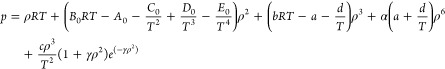
The J–T effect can be described by means of the J–T coefficient, which is the partial derivative of temperature with respect to pressure at constant enthalpy. For a pure component i, the isenthalpic J–T coefficient can be expressed as follows
| 1 |
where μi is the J–T coefficient of pure component i; T is the temperature; p is the pressure; and the subscript H denotes an isenthalpic process. The thermodynamic parameters use SI units unless otherwise specified.
Based on the relation of thermodynamic parameters, eq 1 can be reformulated as
| 2 |
where cp is the molar specific heat capacity of component i at constant pressure.
Equation 2 can be further rearranged as7 follows (see the Supporting Information)
| 3 |
where υ is the molar volume. The term  in eq 3 can be written as
 |
4 |
Substituting eq 4 and the relation between molar volume and molar density υ = 1/ρ into eq 3, the following J–T coefficient of component i can be obtained
| 5 |
It should be noted that eq 5 represents the J–T coefficient of the natural gas mixture provided that the parameters ρ and cp in eq 5 adopt the values of the natural gas mixture. For calculation convenience, accuracy, and efficiency in engineering practice, the J–T coefficient can also be predicted by the pressure–enthalpy chart, empirical formulas, and molecular simulation. To comprehensively explore the influences of hydrogen blending on the J–T coefficient of the natural gas–hydrogen mixture, in this study, one widely used empirical formula and three commonly used EOSs in engineering practice, i.e., SRK-EOS, PR-EOS, and BWRS-EOS, are chosen as representatives to calculate the J–T coefficient of the natural gas–hydrogen mixture.
2.2. Joule–Thomson Coefficient by the Empirical Formula
In an empirical formula, the J–T coefficient of the natural gas–hydrogen mixture is closely related to critical parameters, reduced parameters, and the molar specific heat capacity at constant pressure. The following presents a widely used empirical formula for calculating the J–T coefficient7
| 6 |
where f(pr,Tr) = 2.343Tr–2.04 – 0.071pr + 0.0568; Tr and pr are the reduced temperature and pressure, respectively; Tc and pc denote the critical temperature and pressure, respectively; and cp is the molar specific heat capacity of a gas at constant pressure. For the mixture of natural gas and hydrogen, the parameters in eq 6 are those of the natural gas–hydrogen mixture.
2.3. Joule–Thomson Coefficient by SRK-EOS
SRK-EOS25 is a cubic-type equation of state that has been widely used in natural gas engineering in the past. It is a modification of RK-EOS26 by correcting the a/√T term of RK-EOS using a function α involving the temperature and the acentric factor
| 7 |
where p is the system pressure,
kPa; T is the system temperature, K; υ is the
molar volume, m3/kmol; R is the universal
gas constant, R = 8.3145 kJ/(kmol·K); the attraction
parameter a = a(Tc)α, where  and
and  ;
;  ; Tc and pc are the
critical temperature and critical pressure, respectively; Tr is the reduced temperature,
; Tc and pc are the
critical temperature and critical pressure, respectively; Tr is the reduced temperature,  ; and κ = 0.48508 + 0.55171ω
– 0.15613ω2, where ω is the acentric
factor.
; and κ = 0.48508 + 0.55171ω
– 0.15613ω2, where ω is the acentric
factor.
For the natural gas–hydrogen mixture, the above coefficients a and b in eq 7 are obtained by mixing the corresponding coefficients of included components. The commonly used mixing rules are defined as follows
| 8 |
where C is the total number of components; yi is the mole fraction of component i; and kij is the binary interaction coefficient between components i and j, kij =kji and kii = 0. The value of kij for different components can be obtained in refs (7, 27).
For the convenience of calculation, the molar volume υ in eq 7 can be expressed by molar density. Substituting υ = 1/ρ into eq 7 yields
| 9 |
According to eq 5, the partial derivative of SKR-EOS (eq 9) to temperature T and density ρ should be derived to calculate the J–T coefficient of the natural gas mixture. However, it should be pointed out that the attraction parameter a of SRK-EOS is a function of system temperature T; thus, special attention should be paid to the partial derivative of SRK-EOS, eq 9, to T
| 10 |
| 11 |
where  .
.
Substituting eqs 10 and 11 into eq 5 yields the J–T coefficient μSRK of the natural gas–hydrogen mixture by SRK-EOS.
2.4. Joule–Thomson Coefficient by PR-EOS
Similar to SRK-EOS, PR-EOS is a kind of cubic equation of state developed in 1976 at the University of Alberta by Peng and Robinson.28 It is commonly used to describe the state of natural gas and can be written as follows
| 12 |
where p is the
system pressure,
kPa; T is the system temperature, K; υ is the
molar volume, m3/kmol; the attraction parameter  , where
  ;
;  ; Tc and pc are the
critical temperature and critical pressure, respectively; κ
= 0.37464 + 1.54226ω – 0.26992ω2, where
ω is the acentric factor defined as
; Tc and pc are the
critical temperature and critical pressure, respectively; κ
= 0.37464 + 1.54226ω – 0.26992ω2, where
ω is the acentric factor defined as  ; Tb is the boiling temperature; and patm denotes the atmospheric pressure.
For the natural gas–hydrogen mixture, the mixing rules of PR-EOS for calculating parameters a and b are the same as those of SRK-EOS. However, it should be noted that the binary interaction coefficient kij for PR-EOS is different from that of SRK-EOS.7,27 For the convenience of calculation, the molar volume can be expressed by molar density, and eq 12 can be reformulated as
| 13 |
Similarly, the partial derivative of PR-EOS (eq 13) to temperature T and density ρ can be derived as follows
| 14 |
| 15 |
where  .
.
Finally, substituting eqs 14 and 15 into eq 5 yields the J–T coefficient μPR of the natural gas–hydrogen mixture by PR-EOS.
2.5. Joule–Thomson Coefficient by BWRS-EOS
BWRS-EOS29 is currently the most widely used real gas model for describing the state of natural gas in engineering practice. It is a multiparameter equation of state, which is commonly written as
 |
16 |
where p is the system pressure, kPa; T is the system temperature, K; ρ is the molar density of natural gas, kmol/m3; R is the universal gas constant, R = 8.3145 kJ/(kmol·K); and A0, B0, C0, D0, E0, a, b, c, d, α, and γ are coefficients of BWRS-EOS, which can be calculated based on the critical temperature, critical density, and the acentric factor for a pure component i
 |
17 |
where Ai and Bi are the universal gas constants of component i; ρci is the critical density of component i; and ωi is the acentric factor of component i. The value of the above parameters for different components can be obtained in refs (7, 27).
For the natural gas–hydrogen mixture, the above 11 coefficients of BWRS-EOS are obtained by mixing the corresponding coefficients of included components. The mixing rules are defined by
 |
18 |
where C, yi, and kij have similar meanings as in SRK-EOS and PR-EOS.
Different from SRK-EOS and PR-EOS, the coefficients of BWRS-EOS depend only on the critical parameters and acentric factors, and they have nothing to do with the system temperature and density. Therefore, the partial derivative of BWRS-EOS (eq 16) for natural gas to temperature T and density ρ is the same as that for the pure component. The only distinction is that the coefficients of the partial derivative of BWRS-EOS are obtained according to the mixing rules. The partial derivative of BWRS-EOS for the natural gas–hydrogen mixture to T and ρ can be, respectively, derived as
 |
19 |
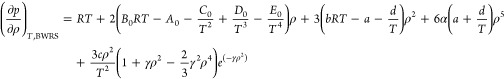 |
20 |
Based on the above analysis, substituting eqs 19 and 20 into eq 5 yields the J–T coefficient μBWRS of the natural gas–hydrogen mixture by BWRS-EOS.
3. Validation
3.1. Experimental Conditions
In this study, the empirical formula, SRK-EOS, PR-EOS, and BWRS-EOS are applied to investigate the influences of hydrogen blending on the J–T coefficient of the natural gas–hydrogen mixture. However, due to the distinctions in model assumption and basic theory, the J–T coefficients calculated by these methods possess different accuracies. Here, the calculation accuracy of the J–T coefficient is validated and analyzed. First, J–T coefficients of three different samples experimentally measured by Ernst et al.16 are used to validate the calculation results of empirical formula, SRK-EOS, PR-EOS, and BWRS-EOS. Table 1 presents the experimental conditions, compositions of sample gases, purity, and mole fraction of each substance in the experiments by Ernst et al.16 In this experiment, the J–T coefficients of pure methane, methane–ethane mixture, and natural gas were measured at various pressures and temperatures. Due to the limitation of the measuring accuracy, the uncertainty of the mole fraction of different substances is also provided in Table 1.
Table 1. Compositions of Investigated Samples16.
| sample | substance | purity | mole fraction |
|---|---|---|---|
| CH4 | CH4 | 0.999995 | 1 |
| CH4 + C2H6 | CH4 | 0.999995 | 0.84874 ± 0.0001 |
| C2H6 | 0.9995 | 0.15126 ± 0.001 | |
| natural gas | CH4 | 0.99995 | 0.79942 ± 0.00004 |
| C2H6 | 0.9995 | 0.05029 ± 0.00001 | |
| C3H8 | 0.9995 | 0.03000 ± 0.00001 | |
| CO2 | 0.999993 | 0.02090 ± 0.00001 | |
| N2 | 0.999999 | 0.09939 ± 0.00001 |
3.2. Analysis of Validation Results
The
J–T coefficients of three investigated samples in Table 1 are calculated using
empirical formula (EF), SRK-EOS, PR-EOS, and BWRS-EOS at different
experimental temperatures and pressures. The calculation results are
compared with the experimental measurement data (EX) from Ernst et
al.,16 and the relative error e between calculation results and the experimental data is also obtained
(e is defined as  ), as shown
in Figures 1–3 and Tables 2–4.
), as shown
in Figures 1–3 and Tables 2–4.
Figure 1.

Relative error of the J–T coefficient of CH4 using the empirical formula, SRK-EOS, PR-EOS, and BWRS-EOS compared with the experimental data.16
Figure 3.

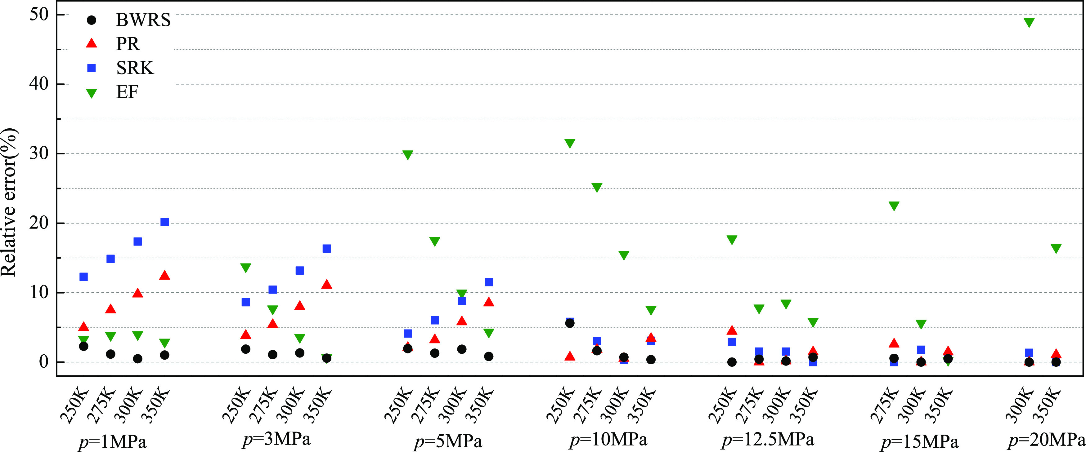
Relative error of the J–T coefficient of the natural gas mixture using the empirical formula, SRK-EOS, PR-EOS, and BWRS-EOS compared with the experimental data.16
Table 2. Comparison of J–T Coefficients of CH4.
| experiment | empirical formula |
SRK-EOS |
PR-EOS |
BWRS-EOS |
||||||
|---|---|---|---|---|---|---|---|---|---|---|
| p (MPa) | T (K) | μEX (K/MPa) | μEF (K/MPa) | eEF (%) | μSRK (K/MPa) | eSRK (%) | μPR (K/MPa) | ePR (%) | μBWRS (K/MPa) | eBWRS (%) |
| 1.0 | 250 | 6.139 | 6.621 | 7.85 | 7.205 | 17.36 | 6.819 | 11.08 | 6.276 | 2.23 |
| 275 | 5.155 | 5.443 | 5.59 | 6.067 | 17.69 | 5.744 | 11.43 | 5.150 | 0.10 | |
| 300 | 4.354 | 4.518 | 3.77 | 5.147 | 18.21 | 4.874 | 11.94 | 4.285 | 1.58 | |
| 350 | 3.085 | 3.200 | 3.73 | 3.763 | 21.98 | 3.565 | 15.56 | 3.058 | 0.88 | |
| 3.0 | 250 | 6.013 | 5.777 | 3.92 | 6.796 | 13.02 | 6.580 | 9.43 | 6.193 | 2.99 |
| 275 | 5.012 | 4.896 | 2.31 | 5.657 | 12.87 | 5.474 | 9.22 | 5.048 | 0.72 | |
| 300 | 4.193 | 4.131 | 1.48 | 4.765 | 13.64 | 4.613 | 10.02 | 4.178 | 0.36 | |
| 350 | 2.958 | 2.962 | 0.14 | 3.455 | 16.80 | 3.351 | 13.29 | 2.954 | 0.14 | |
| 5.0 | 250 | 5.710 | 4.898 | 14.22 | 6.204 | 8.65 | 6.138 | 7.50 | 5.942 | 4.06 |
| 275 | 4.781 | 4.349 | 9.04 | 5.168 | 8.09 | 5.098 | 6.63 | 4.840 | 1.23 | |
| 300 | 3.994 | 3.752 | 6.06 | 4.351 | 8.94 | 4.293 | 7.49 | 4.000 | 0.15 | |
| 350 | 2.811 | 2.733 | 2.77 | 3.153 | 12.17 | 3.119 | 10.96 | 2.817 | 0.21 | |
| 10.0 | 250 | 4.048 | 3.097 | 23.49 | 3.959 | 2.20 | 4.051 | 0.07 | 4.066 | 0.44 |
| 275 | 3.713 | 3.192 | 14.03 | 3.686 | 0.73 | 3.748 | 0.94 | 3.736 | 0.62 | |
| 300 | 3.244 | 2.920 | 9.99 | 3.249 | 0.15 | 3.306 | 1.91 | 3.236 | 0.25 | |
| 350 | 2.353 | 2.214 | 5.91 | 2.443 | 3.82 | 2.504 | 6.42 | 2.384 | 1.32 | |
| 15.0 | 250 | 2.043 ± 0.01 | 2.649 | 29.03 | 2.036 | 0.00 | 2.095 | 2.05 | 2.083 | 1.46 |
| 275 | 2.389 | 2.553 | 6.86 | 2.299 | 3.77 | 2.361 | 1.17 | 2.360 | 1.21 | |
| 300 | 2.327 | 2.358 | 1.33 | 2.239 | 3.78 | 2.307 | 0.86 | 2.285 | 1.80 | |
| 350 | 1.854 | 1.789 | 3.51 | 1.833 | 1.13 | 1.915 | 3.29 | 1.822 | 1.73 | |
| 17.5 | 275 | 1.82 ± 0.03 | 2.397 | 29.57 | 1.788 | 0.61 | 1.837 | 0.00 | 1.846 | 0.00 |
| 300 | 1.91 ± 0.03 | 2.166 | 11.65 | 1.828 | 2.77 | 1.889 | 0.00 | 1.874 | 0.32 | |
| 20.0 | 300 | 1.544 ± 0.023 | 2.011 | 28.33 | 1.489 | 2.10 | 1.538 | 0.00 | 1.536 | 0.00 |
| 350 | 1.398 ± 0.021 | 1.445 | 1.83 | 1.346 | 2.25 | 1.418 | 0.00 | 1.350 | 1.96 | |
| eave | 9.43 | 8.03 | 5.89 | 1.07 | ||||||
Table 4. Comparison of J–T Coefficients of Natural Gas.
| experiment | empirical formula |
SRK-EOS |
PR-EOS |
BWRS-EOS |
||||||
|---|---|---|---|---|---|---|---|---|---|---|
| p (MPa) | T (K) | μEX (K/MPa) | μEF (K/MPa) | eEF (%) | μSRK (K/MPa) | eSRK (%) | μPR (K/MPa) | ePR (%) | μBWRS (K/MPa) | eBWRS (%) |
| 1.0 | 250 | 6.922 | 7.704 | 11.30 | 7.767 | 12.25 | 7.372 | 6.50 | 7.017 | 1.37 |
| 275 | 5.671 | 6.328 | 11.59 | 6.524 | 14.97 | 6.174 | 8.87 | 5.688 | 0.30 | |
| 300 | 4.743 | 5.245 | 10.58 | 5.512 | 16.17 | 5.216 | 9.97 | 4.685 | 1.22 | |
| 350 | 3.333 | 3.703 | 11.10 | 4.013 | 20.31 | 3.791 | 13.74 | 3.293 | 1.20 | |
| 3.0 | 250 | 6.841 | 6.564 | 4.05 | 7.356 | 7.59 | 7.146 | 4.46 | 6.883 | 0.61 |
| 275 | 5.511 | 5.610 | 1.80 | 6.078 | 10.32 | 5.898 | 7.02 | 5.553 | 0.76 | |
| 300 | 4.585 | 4.750 | 3.60 | 5.102 | 11.23 | 4.941 | 7.76 | 4.555 | 0.65 | |
| 350 | 3.205 | 3.411 | 6.43 | 3.656 | 14.20 | 3.562 | 11.14 | 3.178 | 0.84 | |
| 5.0 | 250 | 6.431 | 5.381 | 16.33 | 6.691 | 4.03 | 6.653 | 3.45 | 6.524 | 1.45 |
| 275 | 5.241 | 4.898 | 6.54 | 5.533 | 5.51 | 5.484 | 4.64 | 5.284 | 0.82 | |
| 300 | 4.339 | 4.269 | 1.61 | 4.633 | 6.71 | 4.591 | 5.81 | 4.340 | 0.02 | |
| 350 | 3.032 | 3.130 | 3.23 | 3.321 | 9.50 | 3.310 | 9.17 | 3.024 | 0.26 | |
| 10.0 | 250 | 4.082 | 3.238 | 20.68 | 3.903 | 4.46 | 4.050 | 0.78 | 3.948 | 3.28 |
| 275 | 3.851 | 3.443 | 10.59 | 3.769 | 1.58 | 3.898 | 1.22 | 3.862 | 0.29 | |
| 300 | 3.436 | 3.244 | 5.59 | 3.367 | 1.92 | 3.468 | 0.93 | 3.406 | 0.87 | |
| 350 | 2.504 | 2.504 | 0.00 | 2.533 | 1.04 | 2.629 | 4.99 | 2.495 | 0.36 | |
| 15.0 | 250 | 1.774 ± 0.012 | 2.980 | 66.85 | 1.813 | 1.34 | 1.916 | 7.28 | 1.864 | 4.37 |
| 275 | 2.283 ± 0.011 | 2.817 | 22.80 | 2.214 | 2.73 | 2.318 | 1.05 | 2.270 | 0.09 | |
| 300 | 2.358 ± 0.012 | 2.612 | 10.21 | 2.235 | 4.94 | 2.337 | 0.38 | 2.293 | 2.26 | |
| 350 | 1.926 ± 0.010 | 2.007 | 3.67 | 1.846 | 2.92 | 1.978 | 2.17 | 1.892 | 1.25 | |
| 20.0 | 300 | 1.520 ± 0.015 | 2.249 | 46.51 | 1.423 | 5.65 | 1.509 | 0.00 | 1.492 | 0.86 |
| 350 | 1.417 ± 0.014 | 1.614 | 12.79 | 1.334 | 5.69 | 1.439 | 0.56 | 1.372 | 2.21 | |
| eave | 13.08 | 7.50 | 5.09 | 1.15 | ||||||
Figure 2.
Relative error of the J–T coefficient of the CH4–C2H6 mixture using the empirical formula, SRK-EOS, R-EOS, and BWRS-EOS compared with the experimental data.16
Table 3. Comparison of J–T Coefficients of the CH4 + C2H6 Mixture.
| experiment | empirical formula |
SRK-EOS |
PR-EOS |
BWRS-EOS |
||||||
|---|---|---|---|---|---|---|---|---|---|---|
| p (MPa) | T (K) | μEX (K/MPa) | μEF (K/MPa) | eEF (%) | μSRK (K/MPa) | eSRK (%) | μPR (K/MPa) | ePR (%) | μBWRS (K/MPa) | eBWRS (%) |
| 1.0 | 250 | 7.66 | 7.912 | 3.29 | 8.602 | 12.27 | 8.040 | 4.96 | 7.835 | 2.28 |
| 275 | 6.251 | 6.492 | 3.86 | 7.178 | 14.86 | 6.720 | 7.50 | 6.323 | 1.15 | |
| 300 | 5.164 | 5.369 | 3.97 | 6.061 | 17.35 | 5.669 | 9.78 | 5.189 | 0.48 | |
| 350 | 3.662 | 3.768 | 2.89 | 4.399 | 20.15 | 4.114 | 12.34 | 3.625 | 1.01 | |
| 3.0 | 250 | 7.651 | 6.599 | 13.75 | 8.313 | 8.61 | 7.943 | 3.82 | 7.794 | 1.87 |
| 275 | 6.176 | 5.702 | 7.67 | 6.812 | 10.43 | 6.509 | 5.39 | 6.242 | 1.07 | |
| 300 | 5.028 | 4.848 | 3.58 | 5.691 | 13.17 | 5.429 | 7.98 | 5.094 | 1.31 | |
| 350 | 3.507 | 3.484 | 0.66 | 4.082 | 16.34 | 3.894 | 11.04 | 3.527 | 0.57 | |
| 5.0 | 250 | 7.338 | 5.137 | 29.99 | 7.644 | 4.12 | 7.492 | 2.10 | 7.480 | 1.94 |
| 275 | 5.924 | 4.885 | 17.54 | 6.278 | 6.01 | 6.113 | 3.19 | 6.000 | 1.28 | |
| 300 | 4.806 | 4.327 | 9.97 | 5.234 | 8.82 | 5.084 | 5.78 | 4.895 | 1.85 | |
| 350 | 3.354 | 3.208 | 4.35 | 3.742 | 11.51 | 3.639 | 8.50 | 3.381 | 0.81 | |
| 10.0 | 250 | 3.992 ± 0.02 | 2.715 | 31.65 | 3.740 | 5.79 | 3.944 | 0.70 | 3.750 | 5.59 |
| 275 | 4.280 | 3.197 | 25.30 | 4.145 | 3.04 | 4.202 | 1.82 | 4.210 | 1.64 | |
| 300 | 3.789 | 3.200 | 15.54 | 3.804 | 0.29 | 3.809 | 0.53 | 3.816 | 0.71 | |
| 350 | 2.804 | 2.590 | 7.63 | 2.879 | 3.07 | 2.899 | 3.39 | 2.814 | 0.36 | |
| 12.5 | 250 | 2.34 ± 0.012 | 2.770 | 17.77 | 2.423 | 2.89 | 2.456 | 4.42 | 2.346 | 0.00 |
| 275 | 3.103 ± 0.016 | 2.846 | 7.81 | 3.041 | 1.52 | 3.118 | 0.00 | 3.074 | 0.42 | |
| 300 | 3.113 ± 0.016 | 2.833 | 8.52 | 3.045 | 1.52 | 3.092 | 0.16 | 3.092 | 0.16 | |
| 350 | 2.481 | 2.335 | 5.88 | 2.478 | 0.00 | 2.517 | 1.45 | 2.464 | 0.69 | |
| 15.0 | 275 | 2.198 ± 0.015 | 2.714 | 22.64 | 2.202 | 0.00 | 2.270 | 2.58 | 2.225 | 0.54 |
| 300 | 2.445 ± 0.012 | 2.595 | 5.62 | 2.389 | 1.77 | 2.447 | 0.00 | 2.434 | 0.00 | |
| 350 | 2.123 | 2.117 | 0.28 | 2.113 | 0.61 | 2.154 | 1.46 | 2.113 | 0.47 | |
| 20.0 | 300 | 1.52 ± 0.04 | 2.325 | 49.04 | 1.463 | 1.35 | 1.505 | 0.00 | 1.522 | 0.00 |
| 350 | 1.48 ± 0.04 | 1.771 | 16.51 | 1.491 | 0.00 | 1.536 | 1.05 | 1.506 | 0.00 | |
| eave | 12.63 | 6.62 | 4.00 | 1.05 | ||||||
In Figures 1–3, the different colors denote the different methods adopted to calculate the J–T coefficient, and the symbol height stands for the relative error. It can be clearly seen from Figures 1–3 that for all samples, i.e., pure CH4, CH4 + C2H6, and natural gas, the height of BWRS-EOS is the smallest in almost all of the conditions, indicating that the relative error of BWRS-EOS is the smallest, and the J–T coefficient calculated using BWRS-EOS agrees best with the experimental data under the same condition. From Tables 2–4, it is seen that the average relative error eave of the J–T coefficient between BWRS-EOS and the experimental data is only 1.07, 1.05, and 1.15% for the three investigated samples, respectively. It is inferred that BWRS-EOS is the most accurate among these methods in predicting the J–T coefficient. Figures 1–3 and Tables 2–4 also imply that the calculation accuracy of PR-EOS is slightly lower than that of BWRS-EOS, and the average relative error for the three investigated samples is 5.89, 4.0, and 5.09%, respectively. Compared with BWRS-EOS and PR-EOS, SRK-EOS and empirical formula have relatively low calculation accuracies; especially, the average relative error of the empirical formula for the three investigated samples is around 10% on the whole. Furthermore, as the carbon number of the sample increases, the calculation accuracy of the empirical formula decreases obviously.
As with the influences of temperature and pressure on the calculation accuracy, Tables 2–4 demonstrate that for SRK-EOS and PR-EOS, under the same pressure, a higher temperature provides a larger relative error of the J–T coefficient, while at the same temperature, the relative error of the J–T coefficient is much larger at low pressure than that at high pressure. This indicates that SRK-EOS and PR-EOS can provide a much better prediction of the J–T coefficient at high pressure and low temperature. By contrast, the calculated J–T coefficient is more accurate at low-pressure and high-temperature conditions for BWRS-EOS and the empirical formula. Thus, BWRS-EOS and the empirical formula are favorable for predicting the J–T coefficient at low-pressure and high-temperature conditions. But, overall, BWRS-EOS still delivers results of better accuracy compared to the other two EOSs and the empirical formula at the same given pressure and temperature.
Based on the above comparison, it can be concluded that BWRS-EOS is most accurate in predicting the J–T coefficient within a wide range of thermodynamic conditions (a temperature range of 250–350 K and a pressure range of 1–30 MPa), while PR-EOS, SRK-EOS, and the empirical formula can only deliver good results in a limited range of temperature and pressure. Overall, the calculation accuracy of PR-EOS is still acceptable in most practical engineering problems. Although the performance of the empirical formula is not so good, it is much simpler for engineering applications and can save appreciable computation resources. To ensure the completeness of our investigation and reveal the influences of hydrogen blending on the J–T coefficient of the natural gas mixture by different EOSs, all of the above four methods are adopted in the following study.
3.3. Further Validation by the Methane–Hydrogen Mixture at Low Temperature
In Section 3.2, the calculation accuracy of the empirical formula, SRK-EOS, PR-EOS, and BWRS-EOS is validated by the experimentally measured J–T coefficients of three different samples in the work of Ernst et al.16 It should be noted that in the above comparisons, there is no hydrogen in the three samples. To further verify the applied methods for a hydrogen-enriched system, the experimental data of the J–T coefficient of the CH4 + H2 mixture from Randelman and Wenzel30 are used for comparison with our numerical results. In the experiment of ref (30), the purity of hydrogen is 99.97%, with the impurity being predominantly nitrogen. The mole fraction of hydrogen and methane in the mixture is 56.57 and 43.43%, respectively. Interested readers can refer to ref (30) for more experimental details. However, it is worth mentioning that the experimental temperature in ref (30) is very low (around 200 K), and BWRS-EOS is inapplicable at this condition. Thus, in Table 5, only the calculated J–T coefficients of the CH4 + H2 mixture by the empirical formula, SRK-EOS, and PR-EOS are compared with the experimentally measured J–T coefficients in ref (30).
Table 5. Comparison of the J–T Coefficients of the CH4 + H2 Mixture.
| experiment | empirical formula |
SRK-EOS |
PR-EOS |
|||||
|---|---|---|---|---|---|---|---|---|
| p (atm) | T (K) | μEX (K/atm) | μEF (K/atm) | eEF (%) | μSRK (K/atm) | eSRK (%) | μPR (K/atm) | ePR (%) |
| 68.03 | 199.54 | 0.2617 | 0.1979 | 24.38 | 0.2367 | 9.57 | 0.2551 | 2.52 |
| 61.57 | 198.68 | 0.2715 | 0.2100 | 22.65 | 0.2491 | 8.26 | 0.2678 | 1.36 |
| 57.47 | 196.09 | 0.2807 | 0.2330 | 16.99 | 0.2606 | 7.17 | 0.2802 | 0.18 |
| 50.15 | 194.96 | 0.3023 | 0.2379 | 21.30 | 0.2699 | 10.7 | 0.2955 | 2.25 |
| 43.89 | 192.59 | 0.3264 | 0.2553 | 21.78 | 0.2815 | 13.7 | 0.3119 | 4.44 |
| 38.82 | 191.21 | 0.3496 | 0.2690 | 23.05 | 0.3122 | 10.7 | 0.3241 | 7.29 |
| 71.43 | 181.63 | 0.2846 | 0.2283 | 19.78 | 0.2633 | 7.49 | 0.2827 | 0.67 |
| 63.27 | 178.71 | 0.3094 | 0.2491 | 19.49 | 0.2887 | 6.69 | 0.3076 | 0.58 |
| 55.45 | 176.62 | 0.3383 | 0.2694 | 20.37 | 0.2978 | 11.9 | 0.3309 | 2.19 |
| 47.62 | 173.86 | 0.3723 | 0.2934 | 21.19 | 0.3423 | 8.07 | 0.3566 | 4.22 |
| 40.15 | 170.96 | 0.4095 | 0.3200 | 21.86 | 0.3723 | 9.09 | 0.3823 | 6.64 |
| 51.02 | 204.00 | 0.2735 | 0.2169 | 20.69 | 0.2584 | 5.53 | 0.2743 | 0.29 |
| 43.21 | 202.00 | 0.3001 | 0.2349 | 21.73 | 0.2706 | 9.83 | 0.2908 | 3.10 |
| 35.38 | 199.12 | 0.3268 | 0.2564 | 21.54 | 0.2891 | 11.5 | 0.3096 | 5.26 |
| 30.28 | 197.61 | 0.3442 | 0.2703 | 21.47 | 0.3006 | –12.6 | 0.3211 | 6.71 |
| 24.15 | 195.72 | 0.3652 | 0.2883 | 21.06 | 0.3150 | 13.7 | 0.3350 | 8.27 |
| 18.37 | 193.17 | 0.3850 | 0.3326 | 13.61 | 0.3309 | 14.0 | 0.3501 | 9.06 |
| eave | 20.76 | 10.03 | 3.79 | |||||
It can be clearly seen from Table 5 that at the same experimental pressure and temperature, PR-EOS can give a much better prediction of the J–T coefficient than the empirical formula and SRK-EOS. The average relative error of PR-EOS is only −3.79%, which is much smaller than −10.03% of SRK-EOS and −20.76% of the empirical formula. Compared with Tables 2–4, it can also be found in Table 5 that the relative errors of the empirical formula, SRK-EOS, and PR-EOS are all larger than those at a relatively high-temperature range of 250–350 K. Thus, the thermodynamic condition has a significant influence on the calculation accuracy of the applied EOSs and the empirical formula. Overall, the comparisons of the experimental measurement data with the calculated results as shown in Tables 2–5 indicate that PR-EOS and BWRS-EOS are capable of accurately predicting the J–T coefficient, and BWRS-EOS can perform much better if the temperature is not very low (≥250 K in this study).
4. Results and Discussion
In this section, the effects of hydrogen blending on the Joule–Thomson coefficient of the natural gas–hydrogen mixture are discussed in detail.
4.1. Natural Gas–Hydrogen Mixture
Table 6 depicts the components of the natural gas for the study below.7 The J–T coefficients of the natural gas at six different thermodynamic conditions and six different hydrogen blending ratios are calculated and analyzed. According to the transportation condition using natural gas pipelines or pipe networks, the six thermodynamic conditions are, respectively, set as (1) p = 0.1 MPa and T = 283.15 K; (2) p = 1.0 MPa and T = 283.15 K; (3) p = 1.0 MPa and T = 293.15 K; (4) p = 5.0 MPa and T = 293.15 K; (5) p = 5.0 MPa and T = 308.15 K; and (6) p = 10.0 MPa and T = 323.15 K. The six hydrogen blending ratios (mole fraction) are, respectively, set as 5, 10, 15, 20, 25, and 30%.
Table 6. Composition of the Investigated Natural Gas.
| substance | CH4 | C2H6 | C3H8 | i-C4 | n-C4 | i-C5 | n-C5 | n-C6 | n-C7 | n-C8 | N2 | CO2 |
|---|---|---|---|---|---|---|---|---|---|---|---|---|
| mole fraction (%) | 92.45 | 3.64 | 1.37 | 0.16 | 0.13 | 0.20 | 0.05 | 0.05 | 0.09 | 0.02 | 1.30 | 0.54 |
It should be mentioned that the reason why the maximum hydrogen blending ratio is set as 30% is that the present reports in the literature show that when the hydrogen blending ratio is not higher than 30%, the mixed hydrogen does not significantly affect the combustion characteristics of natural gas, and there is no need to reform the domestic gas appliances of end users.31 The hydraulic and thermal characteristics of natural gas pipelines will not be influenced appreciably as well.32,33 Therefore, the upper limit of the hydrogen blending ratio is set as 30% in this study.
4.1.1. Analysis of the Calculated Joule–Thomson Coefficient
Figures 4–7 display the variation of the J–T coefficient of the natural gas–hydrogen mixture at different hydrogen blending ratios and thermodynamic conditions by the empirical formula, SRK-EOS, PR-EOS, and BWRS-EOS, respectively. It can be obviously seen that under the same thermodynamic conditions, the J–T coefficient of the natural gas–hydrogen mixture approximately linearly decreases with the increase of the hydrogen blending ratio. For instance, Figures 4–7 show that the slope of the μJT–H2% curve (the J–T coefficient versus the hydrogen blending ratio) obtained by the empirical formula, SRK-EOS, PR-EOS, and BWRS-EOS is, respectively, −0.066, −0.085, −0.073, and −0.077 (K/MPa)/% at 0.1 MPa and 283.15 K. Moreover, for the same EOS at the thermodynamic conditions of 0.1–5.0 MPa and 283.15–308.15 K, the decrease range of the J–T coefficient against the increase of the hydrogen blending ratio is approximately the same. That is, the slope of the J–T coefficient curve changing with the hydrogen blending ratio is nearly the same, and the curves under different thermodynamic conditions (except for 10 MPa and 323.15 K) are approximately parallel to each other. For example, the slope of the μJT–H2% curve obtained by PR-EOS at 0.1 MPa/283.15 K and 1.0 MPa/283.15 K is −0.073 and −0.074 (K/MPa)/%, respectively. It indicates that the impact of the hydrogen blending ratio on the J–T coefficient is almost the same under different thermodynamic conditions, except for the high-pressure and -temperature conditions, such as 10 MPa and 323.15 K.
Figure 4.

J–T coefficient of the natural gas–hydrogen mixture at different hydrogen blending ratios and thermodynamic conditions calculated using the empirical formula.
Figure 7.

J–T coefficient of the natural gas–hydrogen mixture at different hydrogen blending ratios and thermodynamic conditions calculated using BWRS-EOS.
Figure 5.

J–T coefficient of the natural gas–hydrogen mixture at different hydrogen blending ratios and thermodynamic conditions calculated using SRK-EOS.
Figure 6.

J–T coefficient of the natural gas–hydrogen mixture at different hydrogen blending ratios and thermodynamic conditions calculated using PR-EOS.
In addition, Figures 4–7 also demonstrate that at the same temperature and hydrogen blending ratio, the J–T coefficient of the natural gas–hydrogen mixture decreases with increasing pressure, such as the two curves corresponding to 1.0 and 5.0 MPa at 293.15 K. Similarly, at the same pressure and hydrogen blending ratio, the J–T coefficient of the natural gas–hydrogen mixture decreases with the increase of temperature, such as the two curves corresponding to 293.15 and 308.15 K at 5.0 MPa. Thus, either higher pressure or temperature leads to a smaller J–T coefficient of the natural gas–hydrogen mixture. The hydrogen-mixed natural gas and natural gas without hydrogen (the hydrogen blending ratio is 0% in Figures 4–7) show the same variation trend, implying that hydrogen blending does not affect the variation trend of the J–T coefficient with pressure and temperature. The underlying reason for this phenomenon can be attributed to the influences of temperature and pressure on the physical and thermal properties of the natural gas–hydrogen mixture, such as the density and the specific heat capacity.
To sum up, hydrogen blending has great influences on the J–T coefficient of the natural gas–hydrogen mixture. With the increase of the hydrogen blending ratio, the J–T coefficient of the natural gas–hydrogen mixture decreases approximately linearly. In addition, the decreasing trend of the J–T coefficient with the increasing hydrogen blending ratio is similar under different thermodynamic conditions. In engineering practice, the effect of hydrogen blending on the J–T coefficient is actually a double-edged sword. For example, in pipeline transportation of the natural gas–hydrogen mixture, the influence of hydrogen blending on the J–T coefficient is favorable. Due to this, the J–T coefficient of the natural gas–hydrogen mixture becomes smaller than that of natural gas, the cooling effect is weakened, and thus the risk of gas hydrate blockage at the pipeline valve can be reduced. However, in the liquefaction of hydrogen-enriched natural gas, it is disadvantageous that the J–T cooling of the natural gas–hydrogen mixture is weakened compared with that without hydrogen. Under the same pressure drop, the temperature drop of the natural gas–hydrogen mixture produced by the J–T cooling is lower than that of natural gas without hydrogen. To obtain the same cooling effect, it is necessary to increase the pressure drop, which consumes much more energy. For the convenience of quantitative comparison, Tables 7–10 present detailed data of the J–T coefficient of the natural gas–hydrogen mixture calculated using the empirical formula, SRK-EOS, PR-EOS, and BWRS-EOS at six thermodynamic conditions and six hydrogen blending ratios for reference.
Table 7. J–T Coefficient of the Natural Gas–Hydrogen Mixture Using the Empirical Formula; Unit, K/MPa.
| p/T | 0% | 5% | 10% | 15% | 20% | 25% | 30% |
|---|---|---|---|---|---|---|---|
| 0.1 MPa/283.15 K | 5.85 | 5.60 | 5.17 | 4.84 | 4.51 | 4.18 | 3.87 |
| 1.0 MPa/283.15 K | 5.59 | 5.34 | 4.94 | 4.62 | 4.30 | 3.98 | 3.66 |
| 1.0 MPa/293.15 K | 5.18 | 4.95 | 4.59 | 4.29 | 3.99 | 3.69 | 3.40 |
| 5.0 MPa/293.15 K | 4.19 | 4.01 | 3.74 | 3.48 | 3.21 | 2.93 | 2.63 |
| 5.0 MPa/308.15 K | 3.84 | 3.66 | 3.39 | 3.15 | 2.89 | 2.63 | 2.34 |
| 10 MPa/323.15 K | 2.77 | 2.63 | 2.40 | 2.18 | 1.94 | 1.66 | 1.36 |
Table 10. J–T Coefficient of the Natural Gas–Hydrogen Mixture Using BWRS-EOS; Unit, K/MPa.
| p/T | 0% | 5% | 10% | 15% | 20% | 25% | 30% |
|---|---|---|---|---|---|---|---|
| 0.1 MPa/283.15 K | 5.41 | 5.01 | 4.62 | 4.23 | 3.85 | 3.47 | 3.10 |
| 1.0 MPa/283.15 K | 5.38 | 4.97 | 4.57 | 4.18 | 3.79 | 3.41 | 3.04 |
| 1.0 MPa/293.15 K | 4.98 | 4.60 | 4.23 | 3.86 | 3.50 | 3.15 | 2.80 |
| 5.0 MPa/293.15 K | 4.66 | 4.27 | 3.89 | 3.53 | 3.19 | 2.86 | 2.54 |
| 5.0 MPa/308.15 K | 4.16 | 3.81 | 3.48 | 3.16 | 2.85 | 2.55 | 2.26 |
| 10 MPa/323.15 K | 3.03 | 2.82 | 2.61 | 2.39 | 2.17 | 1.96 | 1.74 |
Table 8. J–T Coefficient of the Natural Gas–Hydrogen Mixture Using SRK-EOS; Unit, K/MPa.
| p/T | 0% | 5% | 10% | 15% | 20% | 25% | 30% |
|---|---|---|---|---|---|---|---|
| 0.1 MPa/283.15 K | 6.43 | 5.99 | 5.56 | 5.13 | 4.71 | 4.29 | 3.87 |
| 1.0 MPa/283.15 K | 6.28 | 5.84 | 5.41 | 4.99 | 4.57 | 4.16 | 3.76 |
| 1.0 MPa/293.15 K | 5.87 | 5.46 | 5.06 | 4.67 | 4.28 | 3.89 | 3.51 |
| 5.0 MPa/293.15 K | 5.01 | 4.67 | 4.33 | 3.99 | 3.67 | 3.35 | 3.03 |
| 5.0 MPa/308.15 K | 4.52 | 4.21 | 3.91 | 3.61 | 3.32 | 3.03 | 2.74 |
| 10 MPa/323.15 K | 3.09 | 2.93 | 2.76 | 2.58 | 2.40 | 2.22 | 2.03 |
Table 9. J–T Coefficient of the Natural Gas–Hydrogen Mixture Using PR-EOS; Unit, K/MPa.
| p/T | 0% | 5% | 10% | 15% | 20% | 25% | 30% |
|---|---|---|---|---|---|---|---|
| 0.1 MPa/283.15 K | 5.99 | 5.60 | 5.22 | 4.85 | 4.48 | 4.13 | 3.79 |
| 1.0 MPa/283.15 K | 5.91 | 5.51 | 5.13 | 4.75 | 4.39 | 4.03 | 3.69 |
| 1.0 MPa/293.15 K | 5.53 | 5.16 | 4.80 | 4.45 | 4.11 | 3.78 | 3.46 |
| 5.0 MPa/293.15 K | 4.92 | 4.56 | 4.22 | 3.89 | 3.58 | 3.28 | 2.98 |
| 5.0 MPa/308.15 K | 4.43 | 4.12 | 3.82 | 3.53 | 3.25 | 2.97 | 2.71 |
| 10 MPa/323.15 K | 3.13 | 2.93 | 2.73 | 2.53 | 2.34 | 2.15 | 1.96 |
4.1.2. Relative Deviation of the Calculated Joule–Thomson Coefficient
To quantitatively reveal the influences of hydrogen blending on the J–T effect of natural gas, the relative deviation between the J–T coefficient of hydrogen-enriched natural gas and that of natural gas without hydrogen is displayed and analyzed in this section. Figures 8–11 show the relative deviation of the J–T coefficient at six thermodynamic conditions and six hydrogen blending ratios calculated using the empirical formula (eEF), SRK-EOS (eSRK), PR-EOS (ePR), and BWRS-EOS (eBWRS), respectively.
Figure 8.

Relative deviation of the J–T coefficient between the hydrogen-blended natural gas and natural gas without hydrogen under different conditions using the empirical formula.
Figure 11.

Relative deviation of the J–T coefficient between the hydrogen-enriched natural gas and natural gas without hydrogen under different conditions using BWRS-EOS.
Figure 9.

Relative deviation of the J–T coefficient between the hydrogen-enriched natural gas and natural gas without hydrogen under different conditions using SRK-EOS.
Figure 10.

Relative deviation of the J–T coefficient between the hydrogen-enriched natural gas and natural gas without hydrogen under different conditions using PR-EOS.
It can be clearly observed from Figures 8–11 that with the increase of the hydrogen blending ratio, the relative deviation of the J–T coefficient between the natural gas–hydrogen mixture and natural gas without hydrogen increases gradually. When the hydrogen blending ratio is up to 30%, the relative deviations of the J–T coefficient calculated using the empirical formula, SRK-EOS, PR-EOS, and BWRS-EOS are as high as 50.9, 40.2, 39.4, and 45.7%, respectively, compared with those of natural gas without hydrogen. This indicates that the hydrogen blending ratio has important impacts on the J–T effect of natural gas. That is to say, when the hydrogen blending ratio reaches 30%, the temperature drop caused by the J–T effect is decreased by 40–50% under the same pressure drop. This phenomenon exerts negative effects on the process of liquefaction of natural gas; the same pressure drop of the hydrogen-blended natural gas can only yield a 50–60% cooling effect compared with that of natural gas without hydrogen. It is suggested that if the end user of the hydrogen-enriched natural gas is a natural gas liquefaction plant, the throttling process that induces the cooling effect should be improved accordingly. For pipeline transportation of the natural gas–hydrogen mixture, it is also essential to carefully consider the impact of hydrogen blending on downstream end users.
4.2. Methane–Hydrogen Mixture
It is worth pointing out that due to the difference in the composition of natural gas produced from different natural gas fields, the J–T coefficient of different natural gas components at different hydrogen blending ratios varies substantially, which is inconvenient for readers to compare and benchmark. Therefore, the J–T coefficient of the methane–hydrogen mixture at different hydrogen blending ratios is presented in this study for readers’ reference and benchmark. Since the prediction result of BWRS-EOS is most accurate, only the J–T coefficient calculated using BWRS-EOS is presented here. Table 11 shows the J–T coefficient of the methane–hydrogen mixture at the hydrogen blending ratios (mole fraction) of 5, 10, 15, 20, 25, and 30%; pressure of 0.5–20 MPa; and a temperature of 275 K. Similarly, the J–T coefficients of the methane–hydrogen mixture at the same hydrogen blending ratios and pressure and temperatures of 300 and 350 K are presented in Tables 12 and 13, respectively.
Table 11. J–T Coefficient of the Methane–Hydrogen Mixture at 275 K; Unit, K/MPa.
| p (MPa) | 5% | 10% | 15% | 20% | 25% | 30% |
|---|---|---|---|---|---|---|
| 0.5 | 4.76 | 4.38 | 4.00 | 3.64 | 3.28 | 2.95 |
| 1.0 | 4.74 | 4.35 | 3.97 | 3.60 | 3.25 | 2.91 |
| 2.0 | 4.69 | 4.28 | 3.89 | 3.52 | 3.16 | 2.82 |
| 3.0 | 4.61 | 4.20 | 3.80 | 3.42 | 3.06 | 2.72 |
| 5.0 | 4.39 | 3.96 | 3.57 | 3.19 | 2.84 | 2.50 |
| 7.5 | 3.96 | 3.56 | 3.19 | 2.84 | 2.51 | 2.20 |
| 10.0 | 3.39 | 3.06 | 2.75 | 2.45 | 2.16 | 1.89 |
| 12.5 | 2.78 | 2.54 | 2.30 | 2.06 | 1.82 | 1.59 |
| 15.0 | 2.23 | 2.07 | 1.89 | 1.71 | 1.52 | 1.33 |
| 17.5 | 1.78 | 1.68 | 1.55 | 1.41 | 1.25 | 1.10 |
| 20.0 | 1.43 | 1.36 | 1.27 | 1.16 | 1.03 | 0.91 |
Table 12. J–T Coefficient of the Methane–Hydrogen Mixture at 300 K; Unit, K/MPa.
| p (MPa) | 5% | 10% | 15% | 20% | 25% | 30% |
|---|---|---|---|---|---|---|
| 0.5 | 3.97 | 3.64 | 3.33 | 3.02 | 2.73 | 2.44 |
| 1.0 | 3.95 | 3.62 | 3.30 | 2.99 | 2.69 | 2.40 |
| 2.0 | 3.89 | 3.55 | 3.23 | 2.91 | 2.61 | 2.33 |
| 3.0 | 3.82 | 3.48 | 3.15 | 2.83 | 2.53 | 2.24 |
| 5.0 | 3.63 | 3.28 | 2.95 | 2.64 | 2.34 | 2.06 |
| 7.5 | 3.31 | 2.98 | 2.66 | 2.37 | 2.09 | 1.82 |
| 10.0 | 2.92 | 2.62 | 2.34 | 2.07 | 1.82 | 1.58 |
| 12.5 | 2.50 | 2.25 | 2.01 | 1.78 | 1.56 | 1.34 |
| 15.0 | 2.09 | 1.90 | 1.70 | 1.51 | 1.32 | 1.13 |
| 17.5 | 1.74 | 1.59 | 1.43 | 1.27 | 1.11 | 0.95 |
| 20.0 | 1.44 | 1.32 | 1.19 | 1.06 | 0.93 | 0.80 |
Table 13. J–T Coefficient of the Methane–Hydrogen Mixture at 350 K; Unit, K/MPa.
| p (MPa) | 5% | 10% | 15% | 20% | 25% | 30% |
|---|---|---|---|---|---|---|
| 0.5 | 2.84 | 2.60 | 2.37 | 2.14 | 1.92 | 1.71 |
| 1.0 | 2.81 | 2.57 | 2.34 | 2.11 | 1.89 | 1.68 |
| 2.0 | 2.76 | 2.52 | 2.28 | 2.05 | 1.83 | 1.62 |
| 3.0 | 2.70 | 2.45 | 2.22 | 1.99 | 1.77 | 1.55 |
| 5.0 | 2.56 | 2.31 | 2.07 | 1.85 | 1.63 | 1.42 |
| 7.5 | 2.35 | 2.11 | 1.88 | 1.66 | 1.50 | 1.25 |
| 10.0 | 2.11 | 1.89 | 1.67 | 1.46 | 1.27 | 1.08 |
| 12.5 | 1.87 | 1.66 | 1.47 | 1.28 | 1.10 | 0.93 |
| 15.0 | 1.63 | 1.45 | 1.27 | 1.10 | 0.94 | 0.78 |
| 17.5 | 1.41 | 1.25 | 1.09 | 0.95 | 0.80 | 0.66 |
| 20.0 | 1.21 | 1.07 | 0.94 | 0.81 | 0.68 | 0.55 |
5. Conclusions
Hydrogen blending has significant influences on the J–T effect of natural gas. In this study, the equation of state of real gas and a widely used empirical formula are applied to numerically investigate the effects of hydrogen blending on the J–T coefficient of a natural gas–hydrogen mixture in detail. The main work and findings of this study can be summarized as follows.
-
(1)
Theoretical formulas for calculating the J–T coefficient of the natural gas–hydrogen mixture using the empirical formula, SRK-EOS, PR-EOS, and BWRS-EOS are mathematically derived. The experimental measurement data of the J–T coefficient of CH4, CH4 + C2H6, natural gas, and CH4 + H2 are used to validate the calculated J–T coefficient using the empirical formula, SRK-EOS, PR-EOS, and BWRS-EOS. Relative errors of the J–T coefficient between the experimentally measured data and these four methods indicate that both PR-EOS and BWRS-EOS are accurate in predicting the J–T coefficient, and BWRS-EOS can perform much better if the temperature is not very low (≥250 K).
-
(2)
The J–T coefficient of natural gas at six different thermodynamic conditions and hydrogen blending ratios is calculated using the empirical formula, SRK-EOS, PR-EOS, and BWRS-EOS, respectively. Results indicate that under different thermodynamic conditions and hydrogen mixing ratios, the J–T coefficient of the natural gas–hydrogen mixture decreases approximately linearly with the increasing hydrogen blending ratio. When the hydrogen blending ratio reaches 30%, the J–T coefficient of the natural gas–hydrogen mixture is 40–50% lower than that of natural gas without hydrogen. In addition, the influence of the hydrogen blending ratio on the J–T coefficient is nearly the same under different thermodynamic conditions.
-
(3)
The database for the J–T coefficient of the methane–hydrogen mixture at 275, 300, and 350 K is presented in this work to provide a reference and a benchmark for interested readers, where the pressure is set as 0.5–20 MPa and the hydrogen blending ratio of 5–30% is taken into account.
This study also demonstrates that the impact of hydrogen blending on the J–T coefficient of natural gas is a double-edged sword. For long-distance pipeline transportation of the natural gas–hydrogen mixture, hydrogen blending can reduce the risk of gas hydrate blockage at the pipeline valves. For natural gas liquefaction, however, the temperature drop of the hydrogen-mixed natural gas is smaller than that of natural gas without hydrogen under the same pressure drop. To produce the same cooling effect, a larger pressure drop is required for the natural gas–hydrogen mixture.
Acknowledgments
This study is supported by the National Natural Science Foundation of China (Nos. 51904031 and 51936001) and the Beijing Municipal Natural Science Foundation (No. 3204038).
Supporting Information Available
The Supporting Information is available free of charge at https://pubs.acs.org/doi/10.1021/acsomega.1c00248.
The authors declare no competing financial interest.
Supplementary Material
References
- Dincer I.; Midilli A.; Hepbasli A.; Karakoc T. H.. Global Warming: Engineering Solutions; Academic Press: Springer, 2010; pp 71–80. [Google Scholar]
- Zhou S. Y.; Sun K. Y.; Wu Z.; Gu W.; Wu G. X.; Li Z.; Li J. J. Optimized operation method of small and medium-sized integrated energy system for P2G equipment under strong uncertainty. Energy 2020, 199, 117269 10.1016/j.energy.2020.117269. [DOI] [Google Scholar]
- Belderbos A.; Valkaert T.; Bruninx K.; Delarue E.; D’haeseleer W. Facilitating renewables and power-to-gas via integrated electrical power-gas system scheduling. Appl. Energy 2020, 275, 115082 10.1016/j.apenergy.2020.115082. [DOI] [Google Scholar]
- Guandalini G.; Campanari S.; Romano M. C. Power-to-gas plants and gas turbines for improved wind energy dispatchability: Energy and economic assessment. Appl. Energy 2015, 147, 117–130. 10.1016/j.apenergy.2015.02.055. [DOI] [Google Scholar]
- Schnuelle C.; Wassermann T.; Fuhrlaender D.; Zondervan E. Dynamic hydrogen production from PV & wind direct electricity supply – Modeling and techno-economic assessment. Int. J. Hydrogen Energy 2020, 45, 29938–29952. 10.1016/j.ijhydene.2020.08.044. [DOI] [Google Scholar]
- Messaoudani Z. L.; Rigas F.; Hamid M. D. B.; Hassan C. R. C. Hazards, Safety and knowledge gaps on hydrogen transmission via natural gas grid: A critical review. Int. J. Hydrogen Energy 2016, 41, 17511–17525. 10.1016/j.ijhydene.2016.07.171. [DOI] [Google Scholar]
- Li Y. X.; Yao G. Z.. Design and Management of Natural Gas Pipeline, 2nd ed.; Academic Press: Dongying, China, 2009; pp 22–42. [Google Scholar]
- Liu W.; Hu J.; Li X.; Sun Z.; Sun F.; Chu H. Assessment of hydrate blockage risk in long-distance natural gas transmission pipelines. J. Nat. Gas Sci. Eng. 2018, 60, 256–270. 10.1016/j.jngse.2018.10.022. [DOI] [Google Scholar]
- Li X.; Liu Y.; Liu Z.; Chu J.; Song Y.; Yu T.; Zhao J. A hydrate blockage detection apparatus for gas pipeline using ultrasonic focused transducer and its application on a flow loop. Energy Sci. Eng. 2020, 8, 1770–1780. 10.1002/ese3.631. [DOI] [Google Scholar]
- Liu Z.; Yang M.; Liu Y.; Song Y.; Li Q. Analyzing the Joule-Thomson effect on wellbore in methane hydrate depressurization with different back pressure. Energy Procedia 2019, 158, 5390–5395. 10.1016/j.egypro.2019.01.625. [DOI] [Google Scholar]
- Qing D. S.; Xu J.; Chi S. G.; Zhou B.; Jian Z. Y.; Yang F.; Gao T. Optimization of the high-pressure ejection process in small-scale natural gas liquefaction plants. Nat. Gas Ind. 2020, 40, 118–125. [Google Scholar]
- Francis P. G.; Mcglashan M. L.; Wormaldsa C. J. A vapour-flow calorimeter fitted with an adjustable throttle. The isothermal Joule-Thomson coefficient of benzene. The temperature-dependence of the second virial coefficient of benzene. J. Chem. Thermodyn 1969, 1, 441–458. 10.1016/0021-9614(69)90003-2. [DOI] [Google Scholar]
- Clarke P. H.; Francis P. G.; George M.; Phutela R. C.; Roberts G. K. S. C. Flow calorimeters for the measurement of the isothermal Joule-Thomson coefficient of benzene and of cyclohexane vapour. J. Chem. Thermodyn. 1979, 11, 125–139. 10.1016/0021-9614(79)90161-7. [DOI] [Google Scholar]
- Francis P. G. A flow calorimeter for the measurement of the heat capacities and Joule-Thomson coefficients of condensable vapours. J. Chem. Thermodyn. 1990, 22, 545–556. 10.1016/0021-9614(90)90146-H. [DOI] [Google Scholar]
- Cuscó L.; McBain S. E.; Saville G. A flow calorimeter for the measurement of the isothermal Joule-Thomson coefficient of gases at elevated temperatures and pressures. Results for nitrogen at temperatures up to 473 K and pressures up to 10 MPa and for carbon dioxide at temperatures up to 500 K and pressures up to 5 MPa. J. Chem. Thermodyn. 1995, 27, 721–733. 10.1006/jcht.1995.0073. [DOI] [Google Scholar]
- Ernst G.; Keil B.; Wirbser H.; et al. Flow-calorimetric results for the massic heat capacity cp and the Joule–Thomson coefficient of CH4, of (0.85 CH4 + 0.15 C2H6), and of a mixture similar to natural gas. J. Chem. Thermodyn. 2001, 33, 601–613. 10.1006/jcht.2000.0740. [DOI] [Google Scholar]
- Vrabec J.; Kumar A.; Hasse H. Joule–Thomson inversion curves of mixtures by molecular simulation in comparison to advanced equations of state: Natural gas as an example. Fluid Phase Equilib. 2007, 258, 34–40. 10.1016/j.fluid.2007.05.024. [DOI] [Google Scholar]
- Figueroa-Gerstenmaier S.; Lísal M.; Nezbeda I.; Smith W. R.; Trejos V. M. Prediction of isoenthalps, Joule–Thomson coefficients and Joule–Thomson inversion curves of refrigerants by molecular simulation. Fluid Phase Equilib. 2014, 375, 143–151. 10.1016/j.fluid.2014.05.011. [DOI] [Google Scholar]
- Zhang D. T.; Teng L.; Li Y. X. A calculation method for Joule-Thomson coefficient of pipeline CO2. Oil Gas Storage Transp. 2018, 37, 35–39. [Google Scholar]
- Tay W. H.; Lau K. K.; Shariff A. M. Numerical simulation for dehydration of natural gas using Joule Thompson cooling effect. Procedia Eng. 2016, 148, 1096–1103. 10.1016/j.proeng.2016.06.600. [DOI] [Google Scholar]
- Haghighi B.; Hussaindokht M. R.; Reza B. M.; Matin N. S. Joule–Thomson inversion curve prediction by using equation of state. Chin. Chem. Lett. 2007, 18, 1154–1158. 10.1016/j.cclet.2007.07.002. [DOI] [Google Scholar]
- Abbas R.; Ihmels C.; Enders S.; Gmehling J. Joule–Thomson coefficients and Joule–Thomson inversion curves for pure compounds and binary systems predicted with the group contribution equation of state VTPR. Fluid Phase Equilib. 2011, 306, 181–189. 10.1016/j.fluid.2011.03.028. [DOI] [Google Scholar]
- Ghanbari M.; Check G. R. New super-critical cohesion parameters for Soave–Redlich–Kwong equation of state by fitting to the Joule–Thomson Inversion Curve. J. Supercrit. Fluids 2012, 62, 65–72. 10.1016/j.supflu.2011.10.010. [DOI] [Google Scholar]
- Regueira T.; Varzandeh F.; Stenby E. H.; Yan W. Heat capacity and Joule-Thomson coefficient of selected n-alkanes at 0.1 and 10 MPa in broad temperature ranges. J. Chem. Thermodyn. 2017, 111, 250–264. 10.1016/j.jct.2017.03.034. [DOI] [Google Scholar]
- Soave G. Equilibrium constants from a modified Redkh-Kwong equation of state. Chem. Eng. Sci. 1972, 27, 1197–1203. 10.1016/0009-2509(72)80096-4. [DOI] [Google Scholar]
- Redlich O.; Kwong J. N. S. On the thermodynamics of solutions. V. An equation of state. Fugacities of gaseous solutions. Chem. Rev. 1949, 44, 233–244. 10.1021/cr60137a013. [DOI] [PubMed] [Google Scholar]
- Li C.; Huang Z.. Pipeline Transport of Natural Gas, 3rd ed.; Academic Press: Beijing, 2016; pp 30–45. [Google Scholar]
- Peng D. Y.; Robinson D. B. A new two-constant equation of state. Ind. Eng. Chem. Fundam. 1976, 15, 59–64. 10.1021/i160057a011. [DOI] [Google Scholar]
- Starling K. E.; Powers J. E. Enthalpy of mixtures by modified BWR equation. Ind. Eng. Chem. Fundam. 1970, 9, 531–537. 10.1021/i160036a002. [DOI] [Google Scholar]
- Randelman R. E.; Wenzel L. A. Joule-Thomson coefficients of hydrogen and methane mixtures. J. Chem. Eng. Data 1988, 33, 293–299. 10.1021/je00053a021. [DOI] [Google Scholar]
- Wang W.; Wang Q.; Deng H.; Cheng G.; Li Y. Feasibility analysis on the transportation of hydrogen–natural gas mixtures in natural gas pipelines. Nat. Gas Ind. 2020, 40, 130–136. [Google Scholar]
- Tabkhi F.; Azzaro-Pantel C.; Pibouleau L.; Domenech S. A mathematical framework for modelling and evaluating natural gas pipeline networks under hydrogen injection. Int. J. Hydrogen Energy 2008, 33, 6222–6231. 10.1016/j.ijhydene.2008.07.103. [DOI] [Google Scholar]
- Huang M.; Wu Y.; Wen X.; Liu W.; Guan Y. Feasibility analysis of hydrogen transport in natural gas pipeline. Gas Heat Ind. 2013, 033, 39–42. [Google Scholar]
Associated Data
This section collects any data citations, data availability statements, or supplementary materials included in this article.