Agriculture and forest land use change in the continental United States: Are there tipping points?

Summary

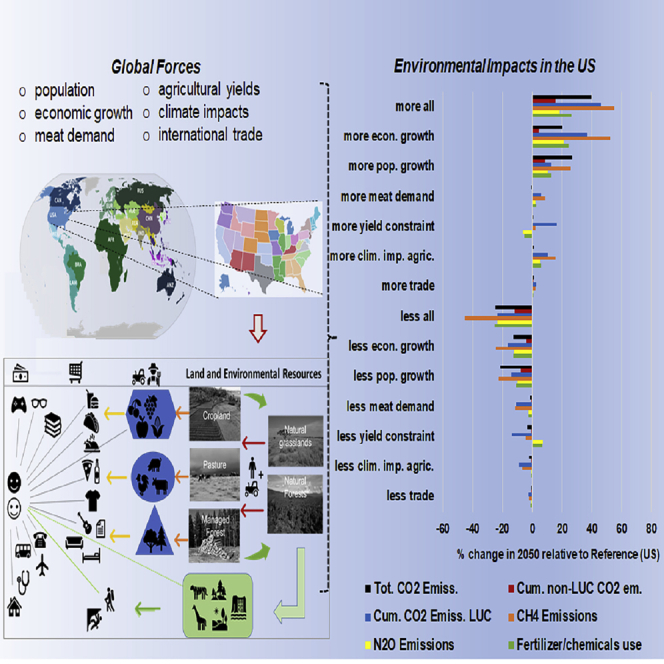
Land use in the United States (US) is driven by multiple forces operating at the global level, such as income and population growth, yield and productivity improvement, trade policy, climate change, and changing diets. Future land use has implications for biodiversity, run-off, carbon storage, ecosystem values, agriculture, and the broader economy. We investigate those forces and their implications from a multisector, multisystem dynamics (MSD) perspective focused on understanding dynamics and resilience in complex interdependent systems. Historical trends show slight increases in grassland and natural forest areas and decreases in cropland. We project these trends to intensify under higher pressures for agriculture land and reduce under lower pressures, with no evidence of tipping points toward larger agricultural land abandonment or deforestation. However, US sectoral output and trade, fertilizer use, N₂O and CH₄ emissions from agriculture activities, and CO₂ emissions from land use changes are substantially impacted under land use forcing scenarios.

Graphical abstract

Highlights

• •Land use changes in the US depend on global economic and environmental pressures
• •Pasture and grassland expand under higher economic and population growth
• •Increase in livestock and fertilizer use brings challenging environmental outcomes
• •Complex systems interactions where resilience in one system shifts forces to others

Earth sciences; Agricultural science; Agricultural economics; Land use.

Introduction

Land use is changed in response to a variety of pressures, with implications for biodiversity, run-off, carbon storage, ecosystem values, agriculture, and the broader economy. Drivers of land use changes include several demand and supply forces, such as increasing population and consumption together with economic and income growth (Alexandratos and Bruinsma, 2012; Bruinsma, 2009; Hertel, 2011; Krausmann et al., 2013; Nelson et al., 2014; Springmann et al., 2018; Van Ittersum et al., 2013), changing diets (Alexandratos and Bruinsma, 2012; Bruinsma, 2009; Springmann et al., 2018; Tilman and Clark, 2014; Weindl et al., 2017), bioenergy demand (Alexandratos and Bruinsma, 2012; Hertel, 2011; Humpenöder et al., 2018; Krausmann et al., 2013), increase in yields (Alexandratos and Bruinsma, 2012; Bruinsma, 2009; Hertel, 2011; Humpenöder et al., 2018; Krausmann et al., 2013; Nelson et al., 2014; Springmann et al., 2018; Stehfest et al., 2019; Van Ittersum et al., 2013; Villoria, 2019a), livestock intensification (Havlík et al., 2014; Weindl et al., 2017), changing international trade patterns (Alexandratos and Bruinsma, 2012; Bruinsma, 2009; Stehfest et al., 2019; Villoria, 2019a; Weindl et al., 2017), climate change (Hertel, 2011; Nelson et al., 2014), land use regulation and land ownership (Humpenöder et al., 2018; Stehfest et al., 2019), and environmental and climate policy (Havlík et al., 2014; Hertel, 2011; Humpenöder et al., 2018). Consequences from land use changes are diverse and affect the overall productive capacity of land to sustain future supplies of both environmental services and primary products to the economies (Foley et al., 2005; Krausmann et al., 2013; Tilman and Clark, 2014).

By far the largest type of land use in the world is agriculture. In the United States (US), agriculture covered 52% of total land areas as of 2012 (Bigelow, 2017). By most accounts, the amount of land used for agriculture in general, and more specifically crops, rose rapidly in the US until about 1930, although data series from the early 1900s and before need careful interpretation because definitions for land types changed (Ramankutty et al., 2010). More recent data are more consistent, especially in the post-World War II period. Since then, land use has been relatively stable over the US as a whole. Rapid yield increases have allowed food production to expand while cropland areas have declined slightly. This has allowed significant areas of forest and natural lands to be maintained or expanded. However, total area in a land use type over a large area can hide significant changes in sub-regions. In the Northeast US, which was heavily farmed and logged in the 1700s and 1800s, with consequently large carbon emissions, much land has returned to forest, whereas more land was converted to agriculture in the center of the country, and along with large irrigation projects in the West. Over the last 50 to 75 years, even those transitions have been limited and land use patterns have been fairly static over much of the country. Cropland area has declined from a high of 155 million hectares (Mha) in the early 1930s to 131Mha (including harvested, failed, summer fallow, and double-cropped areas). Grazing land had also declined from 267Mha in 1945 to 235Mha in the late 1990s, but has rebounded to 265Mha as of 2012 (Bigelow and Borchers, 2017). However, with a ∼370% increase in urban area between 1949 and 2012 (Bigelow and Borchers, 2017), there is a widespread perception of rapid land use change in the US. But with urban land covering only about 3% of the total US land area as of 2012 (Bigelow, 2017), do these perceived changes come from the fact that most people live in cities and witness rapid expansion of urban and built-up areas? Or do these rapid land use changes have the ability to challenge the status quo? Are we at, or near, a tipping point in land use in the US? Is it headed toward land abandonment with reforestation and reintroduction of wildlife in close proximity to urban areas, as happened in the Northeast US, or toward agricultural land expansion? And given the importance of land use in terms of carbon storage, could the position of the US as a net sink for carbon for the past decades (thanks to the reforestation of the East) (Birdsey et al., 2006; Lu et al., 2015) change?

Export-led agricultural growth in the US (and associated land use change) is subject to multiple forces operating at the global level, including income and population growth, trends in yield and productivity improvement, trade policy, climate change, and changing diets. There are debates and uncertainty about the general direction of these forces as it could affect land use globally and in the US (Hertel, 2011). Conventional studies suggest relatively little change in cropland use in the near term to 2050 (Schmitz et al., 2014; Villoria, 2019b). But others have asked whether these various forces operating globally are a perfect storm in the making (Hertel, 2011).

The term “tipping point” has been used in various research fields from climate change to business to describe a situation where a change in a forcer results is a greater than linear response in an outcome (Kiron, 2012; Lenton, 2011). We test this concept with land use change by evaluating whether multiple stressors lead to a greater than additive effect on land use change.

In this study, we approach land use change questions from a multisector MSD perspective focused on understanding dynamics and resilience in complex interdependent systems (Moss et al., 2016). We apply a widely used 18-region, global economic model expanded to include links to natural resources, including energy and land resources. It tracks changes in these resources, maintaining consistent accounts in both value and physical terms, and includes estimates of emissions of pollutants and greenhouse gases from industrial, energy, and land use sources (Chen et al., 2015; Gurgel et al., 2021; Lucena et al., 2016)^, The scenarios are designed to capture the possible divergence in the strength of these global forces from the “BAU” projection based on a review of the literature. For a more complete discussion of the scenario design see Method Details. We also consider the combined set of forces that together would apply the greatest pressure on the US land use (“more” scenarios) or apply the least pressure on the US land use (“less” scenarios) as described in Table 1. The modeling approach is described in Method Details and the model code is available as Data S1.

Table 1.

Scenarios (shocks applied to all regions of the model)

Name	Brief explanation
BAU	Baseline scenario
Less trade	Less trade due to higher import tariffs globally (tariffs 50% higher)
Less clim. imp. Crops	Positive climate impacts on crop yields from GGCMs
Less clim. imp crops&livest.	Positive climate impacts on crop and pasture yields from GGCMs
Less yield constraint	Higher annual increase in crop yields (1.5% per year)
Less meat demand	Changing diets toward lower income elasticity on meat demand
Less pop. growth	Lower population growth (1% lower than “BAU”)
Less econ. growth	Lower GDP growth (20% lower than “BAU”))
Less all	All "less" impacts together
More trade	More trade due to lower import tariffs globally (tariffs 50% lower)
More clim. imp. Crops	Negative climate impacts on crop yields from IPCC local crop models
More clim. imp crops&livest.	Negative climate impacts on crop yields and livestock from IPCC local crop models
More yield constraint	Lower annual increase in crop yields (0.5% per year)
More meat demand	Changing diets toward higher income elasticity on meat demand
More pop. growth	Higher population growth (1% higher than “BAU”))
More econ. growth	Higher GDP growth (20% higher than “BAU”))
More all	All "more" impacts together

Results

We focus on implications for demand of land in the US, considering all complex interdependencies and dynamic relationships among domestic and global demographics, climate, agriculture markets, and economic systems. Figure 1 shows the changes in the major land use categories in the model for all scenarios in 2050 relative to the “BAU” scenario in the US.

Figure 1.

Land use changes in 2050 compared to “BAU” (Mha) in the US

Scenarios with “more” pressures on land use tend to increase the area of pastures and reduce the area of cropland or managed forests in 2050 relative to “BAU”. The “more all” scenario shows the most significant change in land use away from cropland and to pasture and grazing. Including negative climate effects on livestock productivity, more rapid economic and population growth, and a greater bias toward meat consumption as income grows, has the strongest effects on land use transition from crops to pasture. Notably, the total effect of compounding forces in “more all” and “less all” is far less than additive. If the individual forces were purely additive, then summing these reductions in cropland and managed forest across the seven separate “more” scenarios, we would expect a total net change of 77Mha compounding all of the forces. Instead, the total net change in the “more all” scenario is only 43Mha. Compounding the multiple stressors dampens the individual effects because of growing resistance to further reductions in these land use categories, as demand for these commodities and opportunities for intensification on the remaining land are exhausted.

The various “less” scenarios show a consistent reduction in land use change trends from climate change, international trade, meat demand, constraints on yield, population, and gross domestic product (GDP) growth. Compounding all these forces (scenario “less all”), land use changes are restricted to a 22Mha shift from pasture areas to cropland and managed forests by 2050. Surprisingly, this increase in forest areas does not differ much from the forest increase in other scenarios, suggesting that returns to agricultural use and pasture areas are still more attractive in this scenario than the land abandonment to environmental and recreational uses. The overall results show broad resilience in patterns of land use, and no evidence of “tipping points” toward larger reforestation and afforestation in the US in the future, even under lower pressures on global food supply and demand. Similar to the “more” scenarios, the compounding of “less” forces for change (22Mha) is less than additive (67Mha).

Projected land use change from 2012 to 2050 under most scenarios is on the same order as land use change during recent historical periods (Figure 2 and Table S1 in the supplemental information). In recent history, and in projections through 2050, we observe a decline in managed forest and declining or stable levels of cropland, with increasing grazing and pasture, and some increase in natural forest. The “less” scenarios show total net changes in land use of ∼5 to 25Mha. The “more” scenarios have total net changes of ∼30 to 65Mha, closer to the ∼39 to 49Mha in the historical period. In the historical period, newly designated park and wildlife areas contributed to the increase in natural forest area. The projections do not include any new designations of such protected areas.

Figure 2.

Share of land use in the historical period ¹ and in the scenarios “BAU”, “Less All” and “More All” for the continental US

“Forestland grazed” category in ¹ was mapped to Managed Forest in EPPA, “Forestland not grazed” was mapped to Natural Forest in EPPA, and “Grassland” was mapped as Pasture. Rural Parks and Wilderness areas were mapped to Natural Forest in EPPA. Natural Grass in EPPA was added to Pasture.

The land use change pattern in the US since the late 1970s shows a continuous decrease in cropland and forestland grazed areas (which we labeled as “managed forest” in Figure 2 for simplicity) and increase in pasture areas (grassland and pastures in the historical data) and total forestland, as well as other non-agricultural land uses. Other land use change, including rural transportation areas, urban, and defense/industrial lands, increased in the historical period but remains a very small share of land use. We do not attempt to model changes in these uses and include them in the broader “Other” category, along with desert, tundra, and bare rock areas. Relative to total land area in various uses in the continental US, the historical and projected changes are relatively small suggesting a fairly resilient pattern of land use even in the face of significant pressure.

The baseline scenario projects a fairly smooth continuation of historical trends with a net increase in natural forests from 2015 to 2050 of 3.55Mha, which may have relevant implications for biodiversity and soil protection, water regulation, and carbon storage. The cropland contraction under the “BAU” scenario is consistent with other recent projections from the OECD and FAO, which projects a 2.87Mha decrease in cropland in North America by 2028 (OECD-FAO, 2019). Projections generally see reductions in cropland use in developed countries through to 2050 (Bruinsma, 2009; Gurgel et al., 2021).

One explanation for reforestation at the expense of cropland in particular is the “forest transition theory” positing that with economic development a country transitions from a period of forest clearing under low income levels to a reverse movement of agriculture land being abandoned with higher incomes (Rudel, 1998; Rudel et al., 2005). Such changes do not follow a given or deterministic pattern and are a consequence of several forces, such as negative social and ecological impacts, fossil fuel substitution displacing woodfuel, agricultural intensification, land displacement through international trade, and institutional and technological innovations, among others (Gingrich et al., 2019; Lambin and Meyfroidt, 2010). However, some observers see the changing US land use patterns mostly as a geographic shift from cropping in the Eastern US to the West rather than a significant trend toward abandonment nationwide (Ramankutty et al., 2010). There is surprisingly little literature projecting grazing and pasture land or providing a theory for it. However, the change in diet toward more meat consumption with income growth in our “BAU” scenario reflecting historical trends is a likely source. Greater intensity of production on cropland through improved yields has facilitated the reductions in cropland growth that we see according to several authors (Alexandratos and Bruinsma, 2012; Hertel, 2011)^. There has also been a historical trend toward more intensity in livestock production with grain-fed feedlot production replacing grazing and pasture. As noted earlier, that appeared to be a dominant force in the US through the late 1990s with reductions in grazing and pasture areas. Since then, the pattern has reversed, and our projections are consistent with this recent trend reversal. Even a significant shift in diets away from meat does not fully stop the shift from cropland to grazing land. The “less all” scenario eliminates the upward trend in grazing and pastureland but does not reverse it.

Prices are an important indicator of the effects of competing market forces (see Figure 3). The “BAU” projections suggest very stable long run price trajectories for crops, which means no significant change in the relative scarcity of these products in the long run. The trend is for slightly increasing prices for livestock and forestry products. As discussed in the literature, this reflects the faster income growth in emerging economies, together with the changes in diets, toward more consumption of protein from animal origins as income grows. Under the “less” scenarios, particularly with lower population and economic growth, prices of crops decrease in the future while livestock prices increase less or are stable. However, in the “more” scenarios, crop prices increase by up to 50% with more economic growth (less increase for other forces) and livestock prices increasing two-to three-fold, again with economic growth having the biggest effect. Compounding the “more” stressors including negative climate impacts, constraints on improving crop yields, and higher preference for meat (scenario “more all”), leads to steep increases in commodity prices, especially for livestock commodities.

Figure 3.

Global agricultural and food price indexes under alternative scenarios

Table 2 presents percent changes in the US sectoral output, imports and exports by 2050 in all scenarios, relative to those in the “BAU” scenario. Such changes capture the importance of the system dynamics approach, which considers the connections and feedbacks among interdependent and complex human and natural systems. Although our focus here is on future scenarios of land use changes, alternative assumptions about trade, climate impacts on yields, agriculture productivity, changing diets, and population and economic growth, will all affect the sectoral structure and composition of output throughout the economy, and shape relative competitiveness. Some of these forces and stressors (economic, population growth, and trade) affect all sectors. However, as implemented in this study, forces such as climate effects on crop and livestock productivity, yield growth, and meat demand have a direct effect on the agricultural sector and land use, while only indirectly affecting other parts of the economy through the agricultural sector’s demand for other inputs, or through shifting patterns of consumption due to changes in prices. Because the direct effect of some of these forces is mostly on agriculture, we see the strongest effects across all the scenarios in that sector. The US livestock sector experiences the most dramatic changes under the alternative scenarios, followed by the food sector. It means that the comparative advantage of these sectors may change completely depending on the scenario in place. Under the most pressing scenarios (“more all”), livestock production in the US increases by 55% compared to the “BAU” case and exports increase by 520%. Food production and exports are also 69% and 279% higher respectively than in the “BAU” case. Crop production, however, does not increase, so its imports are 77% higher. The effects on exports and imports in percentage terms may seem quite large, but modest changes in output or foreign net demand can lead to large swings in exports and imports, especially when exports are a relatively small share of output. That is the case with baseline exports from the livestock sector, which are very small and mainly in the form of meat and meat products through the food sector. While crop and food exports are six to seven times larger than livestock in the baseline, these results, however, highlight the comparative advantage of the US in the livestock sector.

Table 2.

Changes in the US output, exports and imports in 2050 relative to “BAU” (%)

	Crop			Livestock			Food			Fors&Lum			Energy intensive Ind.			Other Industries
	Output	Export	Import	Output	Export	Import	Output	Export	Import	Output	Export	Import	Output	Export	Import	Output	Export	Import
Less trade	0	−2	−6	−2	−7	−8	−1	−12	−8	1	0	−3	−1	−8	−2	1	0	−5
Less clim. imp. Crops	0	−4	−1	1	0	3	0	−2	0	0	0	0	0	0	0	0	0	0
Less clim. imp crops&livest.	2	−3	−10	−7	−27	−13	−1	−9	−2	0	−3	0	0	2	1	0	1	2
Less yield constraint	13	5	−24	−5	−34	−26	−1	−11	−4	1	−11	3	0	1	2	0	1	2
Less meat demand	2	2	−5	−12	−29	−19	−2	−9	−4	0	−1	0	0	1	1	0	1	1
Less pop. growth	−4	−8	−29	−23	−44	−37	−23	−26	−22	−28	−30	−23	−27	−23	−21	−29	−26	−21
Less econ. growth	−6	−23	−32	−25	−64	−56	−14	−27	−21	−13	−34	−15	−14	−16	−19	−14	−15	−21
Less all	−13	−41	−52	−46	−92	−85	−34	−57	−43	−37	−57	−34	−38	−39	−36	−38	−35	−40
Sum of independent effects	7	−30	−107	−74	−204	−158	−42	−96	−61	−40	−79	−38	−41	−43	−38	−42	−38	−42
More trade	0	2	8	2	7	10	1	14	12	−1	−2	4	4	20	3	−2	−2	6
More clim. imp. Crops	3	13	8	−2	−1	0	0	2	1	0	1	−1	0	−1	−1	0	0	−1
More clim. imp crops&livest.	1	8	16	15	63	27	3	21	5	0	2	−1	−1	−4	−3	−1	−2	−3
More yield constraint	−10	−3	32	3	39	23	1	14	6	−3	6	−3	0	−2	−2	0	−1	−3
More meat demand	−1	−1	5	9	28	20	2	9	4	0	−1	1	0	−1	−1	0	−1	−1
More pop. growth	4	7	44	26	65	48	29	35	28	37	47	28	36	30	25	37	32	23
More econ. growth	7	36	78	54	222	143	21	58	38	15	61	22	16	18	27	16	16	30
More all	1	81	215	55	520	341	69	279	131	47	97	85	57	59	49	57	43	46
Sum of independent effects	0	50	183	109	423	270	57	151	93	48	115	51	55	62	49	51	42	52

	Energy			Refined Oil			Electricity			Services			Construction			Transportation
	Output	Export	Import	Output	Export	Import	Output	Export	Import	Output	Export	Import	Output	Export	Import	Output	Export	Import
Less trade	0	1	−1	−1	−2	−2	0	0	0	0	1	−2	1	3	0	0	1	0
Less clim. imp. Crops	0	0	0	0	0	0	0	1	0	0	0	0	0	0	0	0	0	1
Less clim. imp crops&livest.	1	2	3	−1	1	1	0	1	0	0	2	−1	0	2	0	0	3	1
Less yield constraint	1	3	4	−1	2	2	0	1	0	0	2	−1	0	3	0	0	4	1
Less meat demand	0	1	2	0	1	1	0	1	0	0	1	0	0	2	0	0	2	1
Less pop. growth	−16	−31	−26	−15	−24	−25	−11	−38	−38	−24	−19	−16	−31	−30	−10	−25	−22	−21
Less econ. growth	−13	−26	−22	−6	−18	−18	−7	−24	−20	−14	−9	−21	−13	−11	−8	−13	−10	−20
Less all	−25	−46	−42	−16	−39	−37	−17	−50	−48	−35	−24	−33	−40	−34	−15	−34	−27	−36
Sum of independent effects	−27	−50	−40	−23	−40	−40	−18	−58	−57	−38	−22	−41	−44	−31	−18	−37	−22	−38
More trade	0	−2	0	1	1	1	0	0	1	0	−4	1	−1	−5	−1	0	−4	2
More clim. imp. Crops	0	−1	−1	0	−1	−1	0	0	0	0	−1	0	0	−1	0	0	−1	1
More clim. imp crops&livest.	−1	−4	−4	1	−3	−3	0	−1	−1	0	−3	−1	0	−5	−1	−1	−6	0
More yield constraint	−1	−4	−5	1	−3	−3	0	−2	−1	0	−2	0	0	−4	−1	0	−4	1
More meat demand	0	−1	−2	0	−1	−1	0	0	0	0	−1	−1	0	−2	0	0	−2	1
More pop. growth	20	40	35	17	35	33	27	36	36	32	23	20	43	38	11	32	25	31
More econ. growth	16	36	32	6	28	26	14	20	18	16	3	38	15	5	10	13	0	44
More all	31	54	43	31	52	46	47	51	53	53	14	60	64	12	25	43	−7	95
Sum of independent effects	33	65	57	26	57	52	41	53	54	48	15	57	57	27	19	43	9	79

In terms of compounding stresses, we can, as was done earlier for land use change, compare the sum of changes for the “more” and “less” scenarios simulated independently to the “more all” and “less all” respectively to determine if the effects of multiple forces are more or less than additive. In this regard, we determined whether a scenario was labeled “more” or “less” depending on its impact on land use, our primary research question. That sorting does not necessarily hold when looking at other indicators. For example, less negative climate impact, yield constraint, and meat demand, each lead to increases in crop output in the US, while less population and economic growth lead to lower output of crops. While all of these contribute to less pressure on land, when we compound these forces, we might expect them to be partly offsetting. However, for crops output in the US, the “less all” has a bigger negative impact (−13%) than the sum of the two negative individual impacts. Moreover, the sum of the individual impacts suggests a positive impact on output of 7%. This suggests fairly complex dynamics and interactions among these sectors, moderated through international trade. Outside of the various agriculture sectors, the output effect tends to be close to additive. The compounding effects on exports and imports are often more than additive, indicating that the bulk of the adjustment to changes is through trade. This is not a particularly surprising finding: If output falls, it is more likely that supply of domestic demand will come first and exports will fall more. Or vice versa, if domestic production rises, there is a limit to how much of that can be absorbed by domestic consumption, and so it is more likely that exports will rise disproportionately to the increase in output.

Are there important agriculture-industry interactions? One of the strongest connections, with an important industry-agriculture-environment link, is nitrogen fertilizer use. Various studies have identified this as an important strategy for increasing agricultural output per hectare under land scarcity (Ramankutty et al., 2010), and have attributed as much as 77% of the growth in global crop production that occurred between 1961 and 2005 to increased fertilizer use (Bruinsma, 2009). Although this strategy is well known since the “green revolution”, most of the world’s cropland is not heavily fertilized (Potter et al., 2010) leaving further room for yields improvement. However, such intensification strategy brings environmental concerns including nitrous oxide (N₂O) emissions and eutrophication of water bodies (Vitousek et al., 2009). Among other environmental concerns important to the US agriculture are methane emissions from livestock and CO₂ emissions from land use change. In our analysis, the use of chemicals in agriculture increases by 92% from 2015 to 2050 in the “BAU” scenario. By comparison, crop output grows by 68% in the same period, which means an intensification in the use of these inputs per unit of output in the “BAU”. Figure 4 presents the simulated changes in demand for inputs from “Other Energy-intensive Industries”, which includes the chemicals and fertilizer production, by all agricultural and livestock sectors and its consequential changes in greenhouse gases (GHG) emissions, by the year 2050 (see also Table S6 at supplemental information). The use of fertilizers and chemicals is 10%–20% lower under the “less” scenarios than in the “BAU”, with nitrogen emissions falling equally in both scenarios. However, under the “more” scenarios, fertilizers and chemicals use in agricultural sectors and N₂O emissions increase by 20% or more. Methane emissions follow the same direction, but are more responsive both to lower and higher stressors on land use changes. They increase by more than 50% under the “more all” scenario. The effects of the various forces on cumulative CO₂ emissions from land use change between 2020 and 2050 are intermediate, increasing as much as 40% in the “more all” scenario, and decreasing by nearly 20% in the “less all” scenarios. For comparison purposes, we plot changes in non-land use change CO₂ emissions (from fossil energy combustion and cement production). Those are less responsive than land use and agricultural-related emissions of N₂O and CH_4, which is not surprising given that the “more all” and “less all” scenarios include forces directly affecting the agriculture sector. But even with population and economic growth, which affects the energy and cement sectors directly, the effect on agriculture related emissions is greater. We can conclude that agricultural-related emissions appear more sensitive to these forces than emissions from these other sources.

Figure 4.

Changes (%) in agricultural use of fertilizers and chemical inputs, agricultural sources of N₂O, CH₄, cumulative (2020-2050) CO₂ from land use change (LUC) and total CO₂ from all sources in the US

Discussion

There is a wide range of forces likely to affect land use change in agriculture in the US over the next few decades. These include population and economic growth, changing climate, changing diets, the openness of international trade, and the outlook for yield improvements. Land use in the US has been quite stable over the past several decades, and if anything, cropland area has decreased and more land areas turned into natural areas with additional protections as designated parks and wildlife reserves. Some see the looming multiple forces as the “perfect storm” that could put tremendous new pressure on land use worldwide and in the US, while others have noted slowing population and economic growth rates, and thus project a reduction in pressure on land resources if yield improvements remain at historical rates. The available evidence and opinion on each of these forces varies widely. Some see evidence of plateauing yields, significant yield and productivity loss from climate change, and continued transformation globally toward meat-heavy diets as poorer countries become wealthier. Others see biotechnology as opening up nearly unlimited opportunity for productivity enhancement in agriculture, the rise of non-animal protein options and a move to more plant-based diets, and some studies of climate change see general yield improvements, with the CO₂ fertilization effect on crops and longer growing seasons outweighing any negative effects of drought or extreme heat.

The newly developing research area now referred to as MSD focuses on compounding forces and stressors, the interaction among sectors of the economy and various natural resource systems, and the vulnerability or resilience of systems to these compounding stressors. We developed a set of scenarios as deviations from a business-as-usual scenario that capture the range of results and views on these stressors. The “BAU” scenario is in line with conventional views on agriculture development through 2050, similar in broad trends to projections by the OECD and FAO. We divided these deviations from “BAU” into two groups: One group that includes deviations from the baseline that would increase stress on US land use, and a second group where deviations would reduce it. We evaluated each of these deviations separately, and then all deviations together within each group.

The somewhat surprising conclusion is that we did not find evidence of a strong tipping point toward large deforestation or toward land abandonment even in the scenarios that combined all the forces that would increase stress on land use in the US, or all the forces that would reduce stress. In the “BAU” scenario, we saw a continuation of recent trends in the US—slightly increasing areas in natural forest and a shift to somewhat less cropland and somewhat more pasture and grassland. The “more” and “less” pressure scenarios affected the strength of this shift, but did not reverse it or magnify it dramatically. The scenarios considered in this study allowed us to construct a useful metric for assessing the effect of compounding forces in an MSD setting. We added together the change in a system (e.g., land use) from each of the separate scenarios, and compared that sum to the result when we included all forces together to see how the compounded effect compared to the additive effects. Compounded effects greater than the additive effects would indicate that the system is particularly sensitive to compound stressors, while compounded effects lower than the additive effects would indicate that the interactive forces in the system tend to mute the effects of individual forces when they occur together. For land use, we found that the compounding additional stressor forces were less than 30% of the additive effects, reflecting the basic resilience in land use trends to these forces. However, we observed other results with compounding effects greater than the additive effects: The effect on commodity prices and often on exports. We can trace these effects through all sectors of the economy and can similarly compare the compounding effects to the additive individual effects. However, one should note that: (1) some of the simulated forces primarily affected the agriculture sector directly, and there was limited transmission of the effects outside of the agriculture/land use sectors; (2) Other forces, such as population and economic growth and openness of trade affected the entire economy, creating a very different agriculture sector; (3) Grouping deviations as either more or less pressure on land use did not necessarily mean more pressure on other variables, so the multiple forces tended to work in opposite directions (although when compounded we saw a surprising effects in some cases). An example is crop output under the “less” stress group of effects. Adding the separate effects together would suggest an increase of crop output of 7%, but the compounded effect with all stresses together resulted in crop output decline of 13%. This represents a bigger decline in crop output than if we added together only those forces that separately had a negative effect on crop yield (10%). This result highlights the dynamics and interactions in a complex system. Aside from this study, these simple metrics to determine if compounding forces are additive, less than additive, or perhaps multiplicative, could be useful across the MSD field.

We were also able to track the effect of these forces on emissions of key greenhouse gases. While the relative resilience of land use patterns helped to limit the effect on CO₂ emissions from land use change, the shifts from cropland to pasture and grazing land increased land use CO₂ emissions, more than offsetting the uptake from return to natural land, which was minimal. At the same time, the intensification of crop production to make up for less land in deviations from “BAU” that put more stress on land led to more fertilizer and chemical use and more nitrous oxide emissions. In general, the more stress on land deviations, the more pasture and grassland expansion, reflecting comparative advantage in the US in livestock production, which results in greater methane emissions from livestock. An important conclusion from the MSD perspective is that in complex systems, apparent resilience in one system can shift the forces to other sectors and systems, with consequences for environmental and resource outcomes.

The relative resilience of land use in the US to various stressors may seem somewhat surprising given the wide range of estimates for global and regional future land use in the literature (Nelson et al., 2014; Schmitz et al., 2014; Stehfest et al., 2019). Although results across studies are not easily comparable given the modeling set up, regional coverage, definition of land use categories, and scenario design approach, some broad numbers indicate differences or similarities. For example, a recent model comparison exercise evaluated global land use projections across six models under alternative socio-economic pathways (SSPs) (Stehfest et al., 2019). Comparing alternative SSPs, each individual model estimated between −10% and +10% cropland changes in 2050 going from SSP2 to SSP1 and SSP3, respectively. Only one model achieves −20% and another +18% changes. Detangling the several drivers behind the SSPs, each individual driver (as GDP, population, productivity, and consumption preferences) impacts cropland result in a particular model by less than +5% or −5% in most cases, and in very few cases and models the range of results varies close to −10% or +10%. In our study, cropland area in 2050 varies from −21% to +9% in the US under multiple drivers (or stressors), and from 7% to +9% for individual drivers. At the global level, the range is much smaller, ranging from 4% to +5%. Our range of global land use estimates through 2050 is similar to this recent comparison project, if somewhat narrower.

For the US, similar projections of decreasing cropland areas are found in studies using econometric estimates with fine spatial resolution under alternative policy scenarios (Radeloff et al., 2012), varying assumptions of future crop demand aligned with historical trends (Lawler et al., 2014), and with climate impacts on agricultural prices (Haim et al., 2011). However, these studies projected decreasing pasture and rangeland areas, while most of our scenarios suggest larger pasture areas in the future, consistent with recent trends. A factor that may explain this difference is that those studies did not consider future changes in prices of forage, livestock, and meat products (Haim et al., 2011). The data used to estimate the econometric models covered a relatively short period, 1992 to 1997, when pasture areas were decreasing in the US (Haim et al., 2011; Lawler et al., 2014; Radeloff et al., 2012). However, pasture areas increased after 1997, as they have over the historical period from 1978 to 2012 (Bigelow and Borchers, 2017). Their approach also does not account for general equilibrium effects, as endogenous intensification responses, changes in trade due to growing meat demand outside the US with consequential changes in prices and income, and the US competitive advantage in meat production. These limitations are related to the modeling approach, as they need to sacrifice overall economic balances and consistency in order to represent land use changes at a finer spatial scale.

A further source of uncertainty in the projections is the value of fundamental behavioral parameters in the model. We tested the sensitivity of results to a range of values for the most important behavioral parameters governing land use change. These included: (1) the ability to substitute non-land and land inputs, with greater substitution possibility leading to greater intensification of production on existing land and less need to convert more land (named “intensification elasticity” here); (2) the income elasticity for crops; (3) the land supply elasticity; and (4) the elasticity of substitution between environmental services from natural areas and other goods and services in the welfare function. These parameters are extensively discussed in the literature as key features in determining land use projections (Hertel, 2011).

We change the aforementioned elasticities in the direction of potential higher cropland expansion. The intensification elasticity is reduced by 2/3, from 0.3 to 0.1, which is consistent with observed range of values for corn yield response to prices in the US (Keeney and Hertel, 2009). The income elasticity for crops is kept at the same level as the income elasticity for livestock products, reversing the decreasing trend documented in the literature (Fukase and Martin, 2020; Gouel and Guimbard, 2019). As a result, income elasticity for crops in the US is 0.66 by 2050 in this sensitivity test, instead of 0.24 in the baseline set up of the model. In the case of the land supply elasticity, we increase it five- to six-fold, following estimates for the US of 0.05 for a five-year period and 0.28 for 50 years (Ahmed et al., 2008). The elasticity of substitution between environmental services from natural areas and other goods and services in the welfare function was calibrated too so that historical simulations matched recent trends in land use change, lacking direct estimation of such elasticity in the literature. The baseline calibrated value (0.25) was doubled to 0.5 in the sensitivity test.

The sensitivity results led to changes in land use in the US of less than 5% for many of the parameters (Figure 5). Some exceptions are: (1) under low intensification elasticities, changes in crop and pasture change substantially. In the “BAU” scenario, cropland decrease by 19% and pasture increase by 31% if there is limited room for substituting other inputs for land. These large changes are inconsistent with historical trends, giving more credibility to higher values for the intensification elasticity; (2) For the rest of the world (ROW), the land use results are more sensitive to the assumptions on crop income elasticity. Higher income elasticities increased cropland area by as much as 29% in 2050 in the “more econ. Growth” scenario and reduce pastureland by 17%. In the case of other elasticities, most of them impact land use changes in ROW by less than 10%. An interesting observation from these tests has to do with natural forest and natural grass areas: The only parameter able to affect their results is the land supply elasticity, but only at the rest of the world. Higher land supply elasticities could decrease natural forest areas by 7%–8% in 2050, and natural grass areas by 3%–4%.

Figure 5.

Changes in land use by 2050 in selected scenarios under alternative assumptions on key parameters

In summary, our sensitivity tests for the US and the ROW show some relevant aspects of the agricultural economic modeling framework, which is the representation of farmers’ and consumers’ behavioral responses under land constraints and food scarcity. Crop and livestock intensification practices are common strategies which have increased output per unit area over time, notably when food prices trends show persistent rise. These responses are often ignored in agricultural models dealing primarily with bio-chemical-physical aspects. Under limited possibilities to increase yields by adding more inputs, higher economic growth would require larger areas to raise livestock and grow crops, as shown in our sensitivity tests under low intensification elasticity. As income rises, higher demand for crop and vegetables relate to more sustainable diets in developed countries and among richer households can also impact the projections of future land use trajectories. Otherwise, changes in land use have similar patterns in the US and ROW in all scenarios under alternative modeling assumptions. The most important parameter, which has been a debated response for many decades in the agricultural economics literature, is the intensity elasticity. Annual data often shows little or no significant yield response to commodity price changes, yet within a few years after large price spikes there has typically been a large supply response, suggesting very different short-run and long-run dynamics. As our focus is on the longer-term response, we lean toward a larger intensification elasticity. Our main conclusions regarding the lack of clear tipping points on land use changes in the US in the next decades appears fairly robust, with the chance that changes could be greater if the intensification elasticity is, in fact, very low.

Limitations of the study

From previous discussion, we recognize some caveats and paths for future improvements. Our modeling framework considers environmental and economic interactions through consumption, production, and international markets at global and national levels. It means our results can be considered as “boundary” conditions to the US economy. However, we do not capture local and spatial forces and interplays, which can drive local responses to particular outcomes which are distinct from the national ones. In this way, sub-national impacts on land use changes, greenhouse gas emissions and fertilizer use are not projected in the paper. We aim to improve our analysis in the future by combining an economic model of the US at multi-regional and state levels with several environmental spatialized modeling tools. Other desirable future advancements include the estimation of the intensity elasticity, discussed in previous paragraphs, the modeling of urban land expansion, and the inclusion of climate change impacts on forests.

STAR★Methods

Key resources table

REAGENT or RESOURCE	SOURCE	IDENTIFIER
Deposited Data
Model Code	Gurgel et al. (2021)	Data S1
GTAP8 Database	Narayanan et al. (2012)	https://www.gtap.agecon.purdue.edu/databases/archives.asp
GTAP8 Land Use and Land Cover Database	Baldos and Hertel (2012)	https://www.gtap.agecon.purdue.edu/databases/archives.asp
Energy Sector data	Chen et al. (2015)	https://globalchange.mit.edu/publication/16262
Greenhouse gas emissions and air pollution data	Boden and Andres (2010)	https://www.osti.gov/biblio/1389324
Greenhouse gas emissions and air pollution data	Bond et al. (2007)	https://doi.org/10.1029/2006GB002840
Greenhouse gas emissions and air pollution data	European Commission (2011)	http://edgar.jrc.ec.europa.eu
Greenhouse gas emissions and air pollution data	International Energy Agency (2012)	https://www.iea.org/reports/world-energy-outlook-2012
Short term GDP projections	International Monetary Fund (2019)	https://www.imf.org/external/pubs/ft/weo/2019/02/weodata/index.aspx
Long run GDP projections	Paltsev et al. (2005)	https://globalchange.mit.edu/publication/14578
Cropland and Pasture data	Ramankutty (2011)	http://www.geog.mcgill.ca/∼nramankutty/Datasets/Datasets.html
Natural Land Cover	Felzer et al. (2004)	https://doi.org/10.3402/tellusb.v56i3.16415
Land Supply parameters	Hertel (2011)	https://doi.org/10.1093/ajae/aaq189
Timber value in natural areas	Sohngen (2007)	http://aede.osu.edu/research/forests-and-land-use/global-timber-market-and-forestry-data-project
Parameters of Agricultural CES Functions	Chen et al. (2015)	https://globalchange.mit.edu/publication/16262
Crop yield projections	Gitiaux et al. (2011)	https://globalchange.mit.edu/publication/14009
Crop yield projections	Ray et al. (2013)	https://doi.org/10.1371/journal.pone.0066428
Crop yield projections	Reilly and Fuglie (1998)	https://pubag.nal.usda.gov/download/47776/PDF
Income elasticities for agricultural and food products	Reimer and Hertel (2004)	https://doi.org/10.1080/0953531042000304245
Climate shocks on yields	Gurgel et al. (2021)	https://doi.org/10.1007/s10584-021-03119-8
Software and Algorithms
General Algebraic Modeling System - GAMS	https://www.gams.com/	https://www.gams.com/
Mathematical Programming System for General Equilibrium Analysis - MPSGE	Rutherford (1999)	http://mpsge.org/mainpage/mpsge.htm
Economic Projection and Policy Analysis Model - EPPA	Chen et al. (2015)	https://globalchange.mit.edu/research/research-tools/human-system-model/download
Other
All relevant data and assumptions for modeling	This paper	Properly cited wherever applicable, available in main reference list of the manuscript

Resource availability

Lead contact

Further information and requests for resources should be directed to and will be fulfilled by the Lead Contact, Angelo Gurgel (gurgel@mit.edu).

Materials availability

This study did not generate new unique materials.

Data and code availability

The authors declare that all assumed input data and assumptions are detailed within the article and supplemental information, and were adopted from public resources (literature, public databases, reports etc.) that have been appropriately cited. The model code is included as Data S1. Any extra data and information can be made available by the Lead Contact upon reasonable request.

Method details

Multi-system dynamics modeling approach

Since an initial workshop held in 2016, a new research community focusing on MSD is emerging (Moss et al., 2016). An agreed definition and scope for the field is yet to be developed, but the focus is on environment-human interactions. Traditional modeling approaches aimed at understanding environmental problems and their potential solutions have typically focused on economics, separately from modeling the environment and physical resources. MSD recognizes that environment-human interactions are inevitably complex and interconnected and, therefore, to understand the behavior of these systems, the different modeling approaches need to be merged. The geographic scale and scope of these complex systems can be difficult to define because of global teleconnections in both earth and human systems via, for example, the atmosphere, rivers, and oceans for earth systems, and via trade, communications, travel and population migration for human systems. No man (or woman) is an island, and even an island is not isolated from the effects of changes across the globe.

The dynamics of these complex systems is increasingly important. Standard approaches for addressing risks of extreme events consisted of looking at historical statistics to determine the 100-year flood risk or the frequency of droughts. Even though such events have always been part of a complex interconnected earth system, if the system is variable but within unchanging bounds, then one need not understand the complex system—historical observation could tell you what you needed to know about the magnitude and frequency of extreme events. But with human activity growing and overwhelming natural systems at local, regional, and global levels, historical statistics are no longer a guide to the future. Human activity affecting environmental systems that in turn have feedbacks on human systems means that these various systems are co-evolving.

Why be concerned with trying to understand the coevolution of these complex systems? Ultimately, it is to understand stabilities and instabilities in the systems: Are there tipping points? What forces most affect patterns of development, recognizing interactions of human activity, the built environment, and natural systems? By answering these questions, one can evaluate the resilience of these systems, and provide understanding of how to increase resilience.

While there are a variety of diagrams that have been developed to bring together the concepts of multi-sector or multi-system dynamics, one example is provided in Figure 6. The focus of MSD research includes decision-making frameworks, risks, stressors and influencers such as environmental, demographic and economic change, and other items in the outside ring. It includes consideration of various physical systems such as built infrastructure, natural resources, and material flows listed in the second ring as they interact with various socioeconomic sectors from energy, agriculture, and transportation to manufacturing and services. Finally, the goal of studying these complex linkages is to gain insights into vulnerabilities, tipping points, resilience, and responses to challenges we face in environment-human activity interactions.

Figure 6.

Conceptualizing Multi System Dynamic

The US Global Change Research Program from the outset recognized that systems were complex, multiple forcing and stressors were at play, multi-disciplinary approaches were needed, and local and regional issues were connected to global processes. In that light, MSD is not a completely new idea, but a pulling together of critical concepts that have been found to be important, describing the unique community of multidisciplinary research that has evolved, and laying out the need to further develop these concepts. In the end, MSD questions risk requiring a model of everything. Clearly, boundaries are needed where some forces are exogenous. But a minimum requirement is some representation of both the dynamics of physical systems and human systems and their interaction.

Our exploratory effort aims to investigate the complex interdependent dynamics among multiple systems affecting land use prospects in the US in the next 30 years. We want to test if and under which conditions land use in the US may reach a “tipping point”, or whether land use in a mature economy such as the US is fairly stable. Significant land use change can affect biodiversity, carbon storage, run-off, agricultural production and trade. To examine the potential for tipping points we use a multi-region, multi-sector model of the global economy with a detailed representation of agriculture sectors. The economic model and data are integrated with physical land, energy, and emissions data. The model is able to capture multiple socio-economic and environmental drivers of agricultural and land markets and its interlinkages with the overall economy and land physical resources. It then can simulate the effect of different forces and stressors able to change current uses and trends of land, operating independently or jointly.

Integrated multi-sector, multi system model of forces shaping the US land use

The 18-region global economic model is an extension of the MIT Economic Projection and Policy Analysis model (EPPA), version 6, a recursive-dynamic computable general equilibrium (CGE) model of the world economy (Gurgel et al., 2016, 2021).^2, The economic data is sourced from the Global Trade Analysis Project Version 8 (GTAP 8) database (Narayanan et al., 2012). It provides the base information on social accounting matrices and the structure for regional economies, including bilateral trade flows and energy markets in physical units, and is regularly updated from its original version (Hertel, 1997; Narayanan et al., 2012). The extended version of the model represents 18 regions and 28 sectors. It includes 11 crop and livestock sectors plus a forestry industry, and a number of primary factor inputs (see Table 3). Among them are both depletable and renewable natural capital inputs, as well as produced capital and labor. Among produced capital, EPPA treats cropland, pastures, and managed forest land as “produced” from natural capital of forest areas and grasslands.

Table 3.

Regions, sectors and primary factor inputs

Regions		Sectors		Primary factor inputs
United States	Africa	Rice	Coal	Depletable Natural Capital	Conventional Oil Resources
Canada	Middle East	Maize	Crude Oil		Shale Oil
Mexico	Latin America	Soybean	Refined Oil		Conventional Gas Resources
JAPAN	Rest of Asia	Wheat	Gas		Unconventional Gas Resources
Australia & New Zealand		Sugar Crops	Electricity		Coal Resources
Europe		Vegetables & Fruits	Non-Metallic Minerals	Renewable Natural Capital	Natural Forest
Eastern Europe		Fiber plants	Iron & Steel		Natural Grasslands
Russia		Other crops	Non-Ferrous Metals		Solar and Wind Resources
East Asia		Bovine Cattle	Other Energy-intensive Industries		Hydro Resources
South Korea		Poultry and Pork	Other Industries	Produced Capital	Conventional Capital (Bldgs & Mach.)
Indonesia		Other Livestock	Construction		Cropland
China		Forestry	Other Services		Pasture and Grazing Land
India		Wood Products	Transport		Managed Forest Land
Brazil		Food Products	Ownership of dwellings		Labor

Besides the conventional economic accounts and sectoral data from GTAP, the model includes several alternative energy sectors and detailed transportation choices for households (Chen et al., 2015). Further disaggregation and parameterization of transport and electric power generation go beyond the GTAP base data, taking into account bottom-up engineering analysis of costs, fuel use, and conversion efficiency. The model associates GHG emissions (CO2, CH4, N2O, HFCs, PFCs, and SF6) and conventional air pollutant emissions (SO2, NOx, black carbon, organic carbon, NH3, CO, VOC) with various activities from the combustion of fuels, production cement, waste disposal, and agricultural activities (Boden and Andres, 2010; Bond et al., 2007; European Commission, 2011; International Energy Agency, 2012).^.

The model explicitly treats all inter-industry interactions and bilateral trade in goods. It considers domestic production, exports, imports, government expenditures, investment, and household demand for final goods, and the ownership and supply of labor, capital and natural resources, assuring microeconomic and macroeconomic balances and consistencies. Supplemental accounts link physical quantities of energy (exajoules), emissions (tons), land use (hectares), population (billions of people), natural resource endowments (exajoules, hectares), and efficiencies (energy produced/energy used) of advanced technology with the economic transactions. This treatment captures the physical depletion and use of natural resources, technical efficiencies, and availability of renewable resources. Thus, for example, an increase in population increases the demand for food and other goods and. at the same time, the labor supply. These will cause a cascade of economic and environmental effects, from higher agricultural output and more demand for agricultural land to changes in economic growth and international trade, which are fully accounted for and will lead to a new equilibrium in all markets and economies with a consequent impact on land use and natural resources. Similarly, changing population, trade openness, and crop yields will have cascading effects on food demand, economic growth, and other sectors of the economy.

The model simulates historical economic trajectories recursively to the year 2010 and 2015, and then projects future economic pathways at 5-year intervals from 2015 to 2100. Historical and near-term economic development is benchmarked to IMF’s historical data and short-term GDP projections (International Monetary Fund, 2019) which run through 2018. For later years, we use GDP growth rates (Paltsev et al., 2005), adjusted to reflect long term regional GDP from international institutions as the World Bank and the United Nations (See Table S2 at the supplemental information). The model is formulated using the mixed complementary problems (MCP) approach (Rutherford, 1995), and solved using the MPSGE subsystem in GAMS programming language (Rutherford, 1999).

Future projections are driven by economic growth resulting from savings and investment, and exogenously specified productivity improvement in labor, capital, land, and energy. GDP and income growth through time increase demand for goods and services, including fuels and food. Sectors compete for the available flow of services from renewable resources generating rents. Backstop and advanced technologies may become cost-competitive as regular energy sources become more expensive. These various economic drivers, combined with imposed policies, such as constraints on GHG emissions, determine the economic trajectories over time and across scenarios (the model code is available as Data S1).

Modeling assumptions on land use and land use changes

The economic accounting of land use in the model retains consistency with the supplemental physical accounts on land so that simulated changes in economic use of land translate into hectares of land, preserving total land area constraints in each region. The physical consistency mentioned above is achieved by assuming that one hectare of one type of land is converted to one hectare of another type, and through conversion it takes on the productivity level as the average for that type for that region. The conversion requires using real inputs through a land transformation function (see Figure S2 at the supplemental information). The second consistency is achieved by observing that in equilibrium the marginal conversion cost of land from one type to another should be equal to the difference in value of the types (Gurgel et al., 2016).

The approach considers five broad land use categories: cropland, pasture, forest, natural forest and natural grass. Several world-scale data sources are reconciled for the purpose of this study. These include the GTAP8 Land Use and Land Cover Database (Baldos and Hertel, 2012), which is built from FAOSTAT production data and additional cropland and pasture data (Ramankutty, 2011). Data from the Terrestrial Ecosystem Model (TEM) (Felzer et al., 2004), using historical land use transitions (Hurtt et al., 2006), complements the land use database (Table S4 presents the resulting base year land use and land cover). Land and the transformation of natural lands into managed land types in physical terms is represented (Gurgel et al., 2016). The model considers that through land improvements (draining, tilling, fertilization, and fencing) pastureland can be converted to cropland, or forestland can be harvested, cleared and ultimately used as pastureland or cropland. If investment in cropland is not maintained, the land can then go back to a less intensely managed use (pasture, or forest) or be abandoned completely and returned to “natural” grass or forest land.

The land use transformation approach used in the model is well suited to longer term analysis where demand for some land uses could expand substantially. The approach explicitly represents conversion costs associated with preparing the soil, spreading seeds and managing the creation of a new agricultural system. In this regard, it is a better alternative than the more common Constant Elasticity of Transformation (CET) approach often used in CGE models. The CET function makes large transformations of land difficult because the function tends to preserve input shares (Gurgel et al., 2007). The CET approach also does not explicitly account for conversion costs. In addition, the CET approach does not retain consistent accounting of economic and physical units of land so that you cannot translate a change in the quantity of land use in value terms to a physical change in hectares (Schmitz et al., 2014), an important consideration in tracking land use emission. Finally, as the CET elasticities are symmetric to all changes, the ease of conversion from agricultural to forest land is the same as from forest to agriculture, which implicitly assumes the same “costs” and constraints on conversion in both directions.

In the case of conversion of natural forests, the model accounts for the production of timber products similarly to a forest harvest on managed forest land (see Figure S3 at the supplemental information). Natural areas transformation to agricultural areas are calibrated to mimic a land supply response, based on rates of conversion observed over the last two decades. This last feature captures a variety of factors that may slow land conversion, including increasing costs associated with larger deforestation in a single period and institutional costs (such as limits on deforestation, public pressures for conservation, or establishment of conservation easements or land trusts). The current version of the model is calibrated to a land supply value as reviewed in the literature (Hertel, 2011).

Assuming equilibrium in the base year, conversion costs from one land use category to another as equal to the difference in value of these types, thus assuring “zero profit” conditions in the MCP equilibrium approach. One issue that arises is a value for natural forest and grassland that is not currently used. To appear in the CGE framework it must have an economic value. We develop a “non-use value” for these land areas using data from on timber value on the land (Sohngen and Tennity, 2004; Sohngen, 2007; Sohngen and Mendelsohn, 1998). This approach assumes that, at the margin, the cost of access to remote timber land must equal the value of the standing timber stock plus that of future harvests as the forest regrows. The net present value of the land and timber is calculated using an optimal timber harvest model for each region of the world and for different timber types. Setting the access costs to this value establishes the equilibrium condition that observed current income flow (i.e., rent and returns) from currently non-accessible land is zero because the timber there now, and in the future, can only be obtained by bearing costs to access it equal to its discounted present value. From these data, we calculate the value of an average standing stock of timber for each region and the separate value of the land based on the discounted present value of timber harvests of forest regrowth after the initial harvest of the standing stock.

The value of natural forest and natural grass areas are considered in the model as part of the initial endowment of households in each region. These areas may be converted to other uses or conserved in their natural state. The reservation value of natural lands enters each regional representative agent welfare function with an elasticity of substitution with other consumption goods and services. Hence, the value the agent derives from natural land itself is a deterrent to conversion. Thus, if for example current timber demand rises and puts pressure to harvest more land, it creates a partly offsetting demand to conserve forest area because, implicitly, the agent sees it as more valuable in the future. In the recursive dynamic structure of the model, introducing the natural forest value into the representative agent’s welfare function approximates this behavior. Several applications of previous versions of the EPPA model adopting this land use change approach are available in the literature (Calvin et al., 2014; Gurgel et al., 2011, 2019, 2021; Lucena et al., 2016; Melillo et al., 2009; Reilly et al., 2012; Schmitz et al., 2014; Winchester and Reilly, 2015).

Cropland is an input in the production of each separate crop sector in the model (listed in Table 3). Similarly, pastureland is used in each livestock sector. Managed Forest areas are only used for the production of managed and harvested forests. The land allocation of crop and pasture to the agricultural and livestock sectors is done by CET functions with elasticity equal to one, which is the common approach in all models dealing with broad land categories being allocated to alternative final uses.

Each agricultural sector is modeled by a representative farmer (or firm) who pays for inputs, primary factors, and energy to generate its agricultural product. Inputs are combined in order to maximize profits given technological constraints through a multi-nest Constant Elasticity of Substitution (CES), considering several substitution possibilities in the production function (see Figure S4 and Elasticities of substitution presented in Table S5 of the supplemental information).

Some other features regarding land use changes relate to technological change affecting land productivity and specification of food and agricultural demand. Base parameterization assumes that land is subject to an exogenous productivity improvement of 1% per year for each land type, reflecting assessments of potential productivity improvements showing similar historical crop yields growth, albeit with variations among regions, crops and time (Gitiaux et al., 2011; Ray et al., 2013; Reilly and Fuglie, 1998). In addition to exogenous yield changes and land conversion, agricultural output can grow by intensification of land use through partial substitution of other inputs and other primary factors in the agricultural production functions as relative prices change over time.

Regarding the demand for agricultural, livestock, forestry and food products, most of the output of primary land use sectors end up as inputs in the food, energy, and other sectors of the economy. Food and agriculture production, and hence the amount of land used is strongly influenced by the growth in population and incomes. Most studies find that, as income grows, the expenditure shares on food will decrease although food consumption levels may increase (Haque, 2006; Zhou et al., 2014), which suggests an income elasticity of less than unity. This relationship is represented following the approach using a Stone-Geary preference system (Markusen, 2006), as described below.

The Stone-Geary preference is a Linear Expenditure System (LES), which has a constant marginal budget share for each commodity. The preference system is incorporated by shift parameters for the nested CES expenditure function (Chen et al., 2015). Each shift parameter, which is a subsistence consumption level, changes the reference point of consumption from zero and is calibrated to match estimated regional income elasticities. As a result, for a given set of shift parameters, the limit property of Stone-Geary is still a constant returns to scale (CRTS) function as the CES, and therefore when income increases, we recalibrate shift parameters so the realized income elasticities can approximate the empirically observed levels.

Estimates on final demand income elasticities for agricultural sectors consider an implicit direct additive demand system (Reimer and Hertel, 2004). Since the study of Reimer and Hertel was conducted for the GTAP5 database (which base year is 1997), we adjust those elasticities as functions of income and price levels, to account for changes in economic environment relative to 2007 (see Table S3 in the supplemental information).

The model is able to represent several existing and future pressures on land use, and also the dynamics effects on conversion among alternative agricultural uses, intensification through the use of inputs and capital, and also possible land abandonment, allowing land to revert to natural forms. Scenario exploration analysis allow testing alternative assumptions about population and economic growth, yield and productivity growth, trade and tariffs, climate change, changing patterns of food demand, and land supply behavior.

Some particular aspects of the economic behavior represented in the model are worth further discussion. A major review of global drivers of agricultural land changes identified how these can be summarized into a few economic parameters which, together, determine whether land used for agricultural purposes might increase or decrease (Hertel, 2011). These include: an “elasticity of land supply”, which captures how much agricultural land would expand by conversion of other existing uses given an increase in agricultural land prices; an “intensification elasticity”, measuring how much farmers would increase the use of other inputs (capital, fertilizers, etc.) in response to rising prices for their agricultural products; and an “elasticity of demand”, determining how consumers would react to changes in prices of agricultural products. Together, these parameters will determine how much land will increase under changing conditions of the demand and supply of land, population and income growth, changes in diet patterns, yield and productivity changes due to research achievements, higher input uses or climate change, and so on. All these behavioral parameters are well captured in our socio-economic model and are tested by our exploratory scenarios. As an example, the model explicitly represents land supply elasticity in the conversion of natural forests and natural grasslands to agricultural uses. A review of studies and backward calculations suggests this elasticity may be as low as 0.01 and as high as 0.28 in the US, depending on the time period and modeling issues considered (Hertel, 2011). The base value we use for this parameter for the US is 0.05, consistent with estimated response for a 5-year time frame (Ahmed et al., 2008). We test their upper long-term value of 0.28 later in a sensitivity analysis.

Development of forcing scenarios

We designed a “business as usual” (BAU) and 16 alternative scenarios by varying the strength of various forces and stressors applied to all regions of the world which will likely influence land use in the world and the US (“BAU” projections on economic growth and population and income elasticities for agricultural and food products can be found in the supplemental information, Table S2, Figure S1, and Table S3 respectively). We vary the forcing strength in both directions, labeling as “less” those scenarios that may ease the pressure to expand land use areas for agricultural use or allow conversion back to natural vegetation, and labeling as “more” those scenarios that create greater pressure to convert natural lands to agricultural uses. These forcing changes include those listed in Table 1 in the main text, and expanded on here:

• a)Trade barriers, inducing less trade under higher import tariffs, and more trade under lower barriers (scenarios “less trade” and “more trade”);
• b)Climate impacts on crop yields and livestock productivity, considering average and median impacts from global gridded crop models (GGCMs), usually beneficial to crop yields, and a central value of crop yield impacts varying by region from the Intergovernmental Panel on Climate Change (IPCC) 5^th Assessment report (most negatively affecting yields) (Porter et al., 2014) (scenarios “less clim. imp. Crops” and “more clim.imp. Crops” in which climate impacts are assumed to affect only crops yields, and scenarios “less clim.imp. crops&livest.” and “more clim. imp. crops&livest.” for scenarios affecting crops and pastures yields and livestock productivity) (Gurgel et al., 2021). Climate impacts are represented using estimates from traditional regional-scale studies using site-based models as summarized by the IPCC and global-scale results from GGCMs for four major crops: rice, wheat, maize, and soybean (RMSW), based on results reported in Porter et al. (2014). We calculate a median crop response to climate change by 2050 for each EPPA region for four main crops. The median estimates for each crop span both a variety of crop models and different climate scenarios (Figure S5 in the supplemental information). We extend these impacts to all other crops in the scenario “more clim. imp. crops” and to livestock productivity and pasture yields in the scenario “more clim. imp. crops&livest.” Statistical emulators of the major GGCMs are used to estimate the “less clim. imp. crops” and “less clim. imp. crops&livest.” Two models, pDSSAT and GEPIC, are site-based models applied at the global level, while the three others, LPJ-GUESS, LPJmL and PEGASUS, are global ecosystem models integrating site-based model mechanisms and parameters (Blanc, 2017a, 2017b). They estimate crop yields at a fine resolution (0.5°×0.5° degree) globally by considering the detailed effect of weather (monthly, daily, or even hourly) on crop growth. Similar to the IPPC results, these models are largely limited to four major crops (RMSW). The emulators were used to simulate yields under nine climate scenarios, providing a total of 45 separate simulations for each crop and grid cell. Inputs from the nine scenarios were obtained from the Massachusetts Institute of Technology Integrated Global System Modeling (MIT IGSM) framework using a pattern scaling method (Prinn, 2013) under GHG emissions scenarios consistent with the Paris climate agreement (COP21). The pattern-scaling method uses global scale simulations of the MIT IGSM to estimate the effect of uncertainty in climate sensitivity, ocean heat uptake, and aerosol forcing on latitudinal climate change combined with longitudinal patterns from major general circulation models simulations available through Climate Model Intercomparison Projects (CMIPs). The nine climate scenarios include a high, median, and low climate response to GHG forcing, and three different climate model patterns. We estimate the mean of 45 crop responses simulations for each region for the 2050 period, using a 5-year average yield response for between 2047 and 2052. The central tendency from the IPCC site-based models is for negative effects on yields for nearly all crops and regions, while the central tendencies for the emulated GGCMs results are mostly positive (see Figure S5 in the supplemental information). RMSW are important crops, but account for only 17% of value of the global agriculture production. We extend impacts to other crops by applying the simple average impact of the four main crops in each region to all other crops represented in EPPA. Although it is a simplistic assumption, it avoids an outcome where production is simply shifted to crops that were left unaffected only because no yield estimates were available. Livestock productivity will be directly affected by changes in climate but also indirectly by changes in the price and availability of livestock feed. However, the literature is very scarce on the potential impacts on livestock production and pastures. Given the lack of information, we consider one more subset of scenarios, labelled “Crops & Livestock”, with climate impacts extending to all crops, pasture yields and livestock productivity. Our climate impact scenarios do not include climate impacts on forest growth/yields (or on other sectors such as transportation or human health). Climate impacts on forest productivity are of key importance in determining the full potential of carbon storage, uptake and emissions from land systems (Berner et al., 2017; Büntgen et al., 2019; Kasischke et al., 2013). Here we chose to focus on the food system following the IPCC 5^th Assessment Report (Porter et al., 2014);
• c)Crop yields, assuming a higher rate of increase in exogenous crop yields under lower constraints to research and development and diffusion and the opposite under more constraints (scenarios “less yield constraint” and “more yield constraint”), upper and lower levels in agreement with the literature (Fischer et al., 2014; Ray et al., 2013);
• d)Diets, changing the income elasticity of demand for meat in order to capture a decrease in the preferences for meat in developed countries and no further increase in preferences in developing countries, as also as the opposite trend (scenarios “less meat demand” and “more meat demand”);
• e)Population growth, assuming a lower trend and a higher one (scenarios “less pop. growth” and “more pop. growth”);
• f)Economic growth, testing both a lower and a higher GDP growth rate (scenarios “less econ. Growth” and “more econ.growth”);
• g)The combination of all drivers above, towards less pressure on agricultural land demand, or, conversely, towards more pressure on it (scenarios “less all” and “more all”).

All counterfactual scenarios assume changes in some parameter of the model from its initial calibration point. These cover most of the possible drivers and stressors affecting future land use changes discussed in the literature (Hertel, 2011; Stehfest et al., 2019). To complement the analysis and test the robustness of our results, we also test some alternative parameters governing key behavioral supply and demand responses in the model, as the elasticity of land supply in the US and the world, the degree to which farmers may intensify land use by adding more inputs, the demand income elasticity for crops, and the preference of households for conservation of natural areas. We then verify how these alternative specifications of the model affect the land use projections in 2050 at “BAU”, “more econ. growth” and “less econ. growth” scenarios.

Published: July 23, 2021

Supplemental information

Data S1. Model code

The code contains all data, parameters, assumptions, equations, and scenarios.

References

- Ahmed S.A., Hertel T., Lubowski R. Calibration of a land cover supply function using transition probabilities. GTAP Res. Memo. 2008;14:1–9. [Google Scholar]
- Alexandratos N., Bruinsma J. ESA Work; 2012. World Agriculture towards 2030/2050: The 2012 Revision. Pap. 12. [Google Scholar]
- Baldos U.L.C., Hertel T.W. 2012. Development of a GTAP 8 Land Use and Land Cover Data Base for Years 2004 and 2007. [Google Scholar]
- Berner L.T., Law B.E., Meddens A.J.H., Hicke J.A. Tree mortality from fires, bark beetles, and timber harvest during a hot and dry decade in the western United States (2003-2012) Environ. Res. Lett. 2017;12 doi: 10.1088/1748-9326/aa6f94. [DOI] [Google Scholar]
- Bigelow D.P. 2017. A Primer on Land Use in the United States. [Google Scholar]
- Bigelow D.P., Borchers A. 2017. Major Uses of Land in the United States, 2012. [Google Scholar]
- Birdsey R., Pregitzer K., Lucier A. Forest carbon management in the United States. J. Environ. Qual. 2006;35:1461–1469. doi: 10.2134/jeq2005.0162. [DOI] [PubMed] [Google Scholar]
- Blanc E. Statistical emulators of maize, rice, soybean and wheat yields from global gridded crop models. Agric. For. Meteorol. 2017;236:145–161. doi: 10.1016/j.agrformet.2016.12.022. [DOI] [Google Scholar]
- Blanc E. Aggregation of gridded emulated rainfed crop yield projections at the national or regional level (supplementary files) J. Glob. Econ.Anal. 2017;2:112–127. doi: 10.21642/jgea.020203sm1f. [DOI] [Google Scholar]
- Boden T.A., Andres R.J. 2010. Global, Regional, and National Fossil-Fuel CO2 Emissions. [Google Scholar]
- Bond T.C., Bhardwaj E., Dong R., Jogani R., Jung S., Roden C., Streets D.G., Trautmann N.M. Global Biogeochem.Cycles; 2007. Historical Emissions of Black and Organic Carbon Aerosol from Energy-Related Combustion, 1850-2000. [DOI] [Google Scholar]
- Bruinsma J. Session 2: The Resource Base to 2050: Will There Be Enough Land, Water and Genetic Potential to Meet Future Food and Biofuel Demands? Food and Agriculture Organization of the United Nations (FAO); Rome: 2009. The resource outlook to 2050. By how much do land, water use and cropyields need to increase by 2050? pp. 1–33. [Google Scholar]
- Büntgen U., Krusic P.J., Piermattei A., Coomes D.A., Esper J., Myglan V.S., Kirdyanov A.V., Camarero J.J., Crivellaro A., Körner C. Limited capacity of tree growth to mitigate the global greenhouse effect under predicted warming. Nat. Commun. 2019;10:1–6. doi: 10.1038/s41467-019-10174-4. [DOI] [PMC free article] [PubMed] [Google Scholar]
- Chen Y., Paltsev S., Reilly J., Morris J., Babiker M. The MIT EPPA6 model: economic growth, energy use, and food consumption. MIT Jt. Progr. Sci. Policy Glob. Chang. Rep. 2015:1–45. [Google Scholar]
- Calvin K.V., Beach R., Gurgel A., Labriet M., Loboguerrero Rodriguez A.M. Agriculture, forestry, and other land-use emissions in Latin America. Energy Econ. 2014;56:615–624. doi: 10.1016/j.eneco.2015.03.020. [DOI] [Google Scholar]
- European Commission . 2011. Emission Database for Global Atmospheric Research (EDGAR), Release Version 4.2.http://edgar.jrc.ec.europa.eu [Google Scholar]
- Felzer B., Kicklighter D., Melillo J., Wang C. Tellus B; 2004. Effects of Ozone on Net Primary Production and Carbon Sequestration in the Conterminous United States Using a Biogeochemistry Model. [Google Scholar]
- Fischer T., Byerlee D., Edmeades G. Crop yields and global food security: will copyright Act 1968 yield increase continue to feed the world? Aust. Cent. Int. Agric. Res. 2014:1–634. [Google Scholar]
- Foley J.A., DeFries R., Asner G.P., Barford C., Bonan G., Carpenter S.R., Chapin F.S., Coe M.T., Daily G.C., Gibbs H.K. Global consequences of land use. Science. 2005;309:570–574. doi: 10.1126/science.1111772. [DOI] [PubMed] [Google Scholar]
- Fukase E., Martin W. Economic growth, convergence, and world food demand and supply. World Dev. 2020;132 doi: 10.1016/j.worlddev.2020.104954. [DOI] [Google Scholar]
- Gingrich S., Lauk C., Niedertscheider M., Pichler M., Schaffartzik A., Schmid M., Magerl A., Le Noë J., Bhan M., Erb K. Hidden emissions of forest transitions: a socio-ecological reading of forest change. Curr.Opin. Environ. Sustain. 2019;38:14–21. doi: 10.1016/j.cosust.2019.04.005. [DOI] [Google Scholar]
- Gitiaux X., Reilly J., Paltsev S. 2011. Future Yield Growth: What Evidence from Historical Data? Joint Program Report Series Report 199. [Google Scholar]
- Gouel C., Guimbard H. Nutrition transition and the structure of global food demand. Am. J. Agric. Econ. 2019;101:383–403. doi: 10.1093/ajae/aay030. [DOI] [Google Scholar]
- Gurgel A., Chen Y.-H.H., Paltsev S., Reilly J.M. CGE models: linking natural resources to the CGE framework. In: Dinar A., Bryant W.D.A., editors. Natural Resources and Environmental Policy in the Era of Global Change: Computable General Equilibrium Models. World Scientific Co. Pte. Ltd.; 2016. pp. 57–98. [DOI] [Google Scholar]
- Gurgel A., Cronin T., Reilly J., Paltsev S., Kicklighter D., Melillo J. Food, fuel, forests, and the pricing of ecosystem services. Am. J. Agric. Econ. 2011;93:342–348. doi: 10.1093/ajae/aaq087. [DOI] [Google Scholar]
- Gurgel A.C., Paltsev S., Breviglieri G.V. The impacts of the Brazilian NDC and their contribution to the Paris agreement on climate change. Environ. Dev. Econ. 2019;24:395–412. doi: 10.1017/S1355770X1900007X. [DOI] [Google Scholar]
- Gurgel A.C., Reilly J., Blanc E. Challenges in simulating economic effects of climate change on global agricultural markets. Clim. Change. 2021;166:29. doi: 10.1007/s10584-021-03119-8. [DOI] [Google Scholar]
- Gurgel A., Reilly J.M., Paltsev S. Potential land use implications of a global biofuels industry. J. Agric. Food Ind. Organ. 2007 [Google Scholar]
- Haim D., Alig R.J., Platinga A.J., Sohngen B. Climate change and future land use in the United States: an economic approach. Clim. Chang. Econ. 2011;2:27–51. [Google Scholar]
- Haque M. 2006. Income Elasticity and Economic Development: Methods and Applications. [Google Scholar]
- Havlík P., Valin H., Herrero M., Obersteiner M., Schmid E., Rufino M.C., Mosnier A., Thornton P.K., Böttcher H., Conant R.T. Climate change mitigation through livestock system transitions. Proc. Natl. Acad. Sci. U S A. 2014;111:3709–3714. doi: 10.1073/pnas.1308044111. [DOI] [PMC free article] [PubMed] [Google Scholar]
- Hertel T. 1997. Global Trade Analysis Using the GTAP Model. [Google Scholar]
- Hertel T.W. The global supply and demand for agricultural land in 2050: a perfect storm in the making? Am. J. Agric. Econ. 2011;93:259–275. doi: 10.1093/ajae/aaq189. [DOI] [Google Scholar]
- Humpenöder F., Popp A., Bodirsky B.L., Weindl I., Biewald A., Lotze-Campen H., Dietrich J.P., Klein D., Kreidenweis U., Müller C. Large-scale bioenergy production: how to resolve sustainability trade-offs? Environ. Res. Lett. 2018;13:024011. doi: 10.1088/1748-9326/aa9e3b. [DOI] [Google Scholar]
- Hurtt G., Frolking S., Fearon M., Moore B., Shevliakovas E., Malyshev S., Pacala S.W., Houghton R.A. The underpinnings of land-use history: three centuries of global gridded land-use transitions, wood-harvest activity, and resulting secondary lands. Glob. Chang. Biol. 2006;12:1208–1229. [Google Scholar]
- International Energy Agency . 2012. World Energy Outlook 2012. [Google Scholar]
- International Monetary Fund . 2019. World Economic and Financial Surveys: World Economic Outlook Database.https://www.imf.org/external/pubs/ft/weo/2019/02/weodata/index.aspx [Google Scholar]
- Kasischke E.S., Amiro B.D., Barger N.N., French N.H.F., Goetz S.J., Grosse G., Harmon M.E., Hicke J.A., Liu S., Masek J.G. Impacts of disturbance on the terrestrial carbon budget of North America. J. Geophys. Res. Biogeosciences. 2013;118:303–316. doi: 10.1002/jgrg.20027. [DOI] [Google Scholar]
- Keeney R., Hertel T. The indirect land use impacts of United States biofuel policies: the importance of acreage, yield, and bilateral trade responses. Am. J. Agric. Econ. 2009;91:895–909. [Google Scholar]
- Kiron D. Sustainability nears a tipping point. Strateg.Dir. 2012;28:433. doi: 10.1108/sd.2012.05628gaa.012. [DOI] [Google Scholar]
- Krausmann F., Erb K.H., Gingrich S., Haberl H., Bondeau A., Gaube V., Lauk C., Plutzar C., Searchinger T.D. Global human appropriation of net primary production doubled in the 20th century. Proc. Natl. Acad. Sci. U S A. 2013;110:10324–10329. doi: 10.1073/pnas.1211349110. [DOI] [PMC free article] [PubMed] [Google Scholar]
- Lambin E.F., Meyfroidt P. Land use transitions: socio-ecological feedback versus socio-economic change. Land Use Policy. 2010;27:108–118. doi: 10.1016/j.landusepol.2009.09.003. [DOI] [Google Scholar]
- Lawler J.J., Lewis D.J., Nelson E., Plantinga A.J., Polasky S., Withey J.C., Helmers D.P., Martinuzzi S., Penningtonh D., Radeloff V.C. Projected land-use change impacts on ecosystem services in the United States. Proc. Natl. Acad. Sci. U S A. 2014;111:7492–7497. doi: 10.1073/pnas.1405557111. [DOI] [PMC free article] [PubMed] [Google Scholar]
- Lenton T.M. Early warning of climate tipping points. Nat. Clim. Chang. 2011;1:201–209. [Google Scholar]
- Lu X., Kicklighter D.W., Melillo J.M., Reilly J.M., Xu L. Land carbon sequestration within the conterminous United States: regional- and state-level analyses. J. Geophys. Res. Biogeosci. 2015;120:379–398. doi: 10.1002/2014JG002818. [DOI] [Google Scholar]
- Lucena A.F.P., Clarke L., Schaeffer R., Szklo A., Rochedo P.R.R., Nogueira L.P.P., Daenzer K., Gurgel A., Kitous A., Kober T. Climate policy scenarios in Brazil: a multi-model comparison for energy. Energy Econ. 2016;56:564–574. doi: 10.1016/j.eneco.2015.02.005. [DOI] [Google Scholar]
- Markusen J. University of Colorado; 2006. Extension of the Simple Model.https://spot.colorado.edu/∼markusen/teaching_files/applied_general_equilibrium/GAMS/ch2.pdf [Google Scholar]
- Melillo J.M., Reilly J.M., Kicklighter D.W., Gurgel A.C., Cronin T.W., Paltsev S., Felzer B.S., Wang X., Sokolov A.P., Schlosser C.A. Indirect emissions from biofuels: how important? Science. 2009;326:1397–1399. doi: 10.1126/science.1180251. [DOI] [PubMed] [Google Scholar]
- Moss R., Fisher-Vanden K., Delgado A., Backhaus S., Barrett C.L., Bhaduri B., Kraucunas I.P., Reed P.M., Rice J.S., Wing I.S., Tebaldi C. 2016. Understanding Dynamics and Resilience in Complex Interdependent Systems. [Google Scholar]
- Narayanan B.G., Aguiar A., McDougall R. 2012. Global Trade, Assistance, and Production: The GTAP 8 Data Base. [Google Scholar]
- Nelson G.C., van der Mensbrugghe D., Ahammad H., Blanc E., Calvin K., Hasegawa T., Havlik P., Heyhoe E., Kyle P., Lotze-Campen H. Agriculture and climate change in global scenarios: why don’t the models agree. Agric. Econ. (United Kingdom) 2014;45:85–101. doi: 10.1111/agec.12091. [DOI] [Google Scholar]
- OECD-FAO . 2019. OECD-FAO Agricultural Outlook 2019-2028. [Google Scholar]
- Paltsev S., Reilly J.M., Jacoby H.D., Eckaus R.S., Mcfarland J., Sarofim M., Asadoorian M., Babiker M., No R. Policy Anal. Report; 2005. MIT Joint Program on the Science and Policy of Global Change ( EPPA ) Model : Version 4; p. 78. [Google Scholar]
- Porter J.R., Xie L., Challinor A., Cochrane K., Howden S.M., Iqbal M.M., Lobell D.B., Travasso M. Food security and food production systems. In: Field C.B., editor. Climate Change 2014: Impacts, Adaptation, and Vulnerability. Part A: Global and Sectoral Aspects. Contribution of Working Group II to the Fifth Assessment Report of the Intergovernmental Panel on Climate Change. Cambridge University Press; 2014. pp. 485–533. [Google Scholar]
- Potter P., Ramankutty N., Bennett E.M., Donner S.D. Characterizing the spatial patterns of global fertilizer application and manure production. Earth Interact. 2010;14:1–22. doi: 10.1175/2009EI288.1. [DOI] [Google Scholar]
- Prinn R.G. Development and application of earth system models. Proc. Natl. Acad. Sci. U S A. 2013;110:3673–3680. doi: 10.1073/pnas.1107470109. [DOI] [PMC free article] [PubMed] [Google Scholar]
- Radeloff V., Nelson E., Platinga A.J., Lewis D.J., Helmers D., Lawler J.J., Withey J.C., Beaudry F., Martinuzzi S., Butsic V. Economic-based projections of future land use in the conterminous United States under alternative policy scenarios. Ecol. Applic. 2012;22:1036–1049. doi: 10.1890/11-0306.1. [DOI] [PubMed] [Google Scholar]
- Ramankutty N. 2011. Global Cropland and Pasture Data: 1700-2007.http://www.geog.mcgill.ca/∼nramankutty/Datasets/Datasets.html [Google Scholar]
- Ramankutty N., Heller E., Rhemtulla J. Prevailing myths about agricultural abandonment and forest regrowth in the United States. Ann. Assoc. Am. Geogr. 2010;100:502–512. doi: 10.1080/00045601003788876. [DOI] [Google Scholar]
- Ray D.K., Mueller N.D., West P.C., Foley J.A. Yield trends are insufficient to double global crop production by 2050. PLoS One. 2013;8:e66428. doi: 10.1371/journal.pone.0066428. [DOI] [PMC free article] [PubMed] [Google Scholar]
- Reilly J., Fuglie K. Future yield growth in field crops: what evidence exists? Soil Tillage Res. 1998:275–290. [Google Scholar]
- Reilly J., Melillo J., Cai Y., Kicklighter D., Gurgel A., Paltsev S., Cronin T., Sokolov A., Schlosser A. Using land to mitigate climate change: hitting the target, recognizing the trade-offs. Environ. Sci. Technol. 2012;46:5672–5679. doi: 10.1021/es2034729. [DOI] [PubMed] [Google Scholar]
- Reimer J., Hertel T. Estimation of international demand behaviour for use with input-output based data. Econ. Syst. Res. 2004;16:347–366. [Google Scholar]
- Rudel T.K. Is there a forest transition? Deforestation, reforestation, and development. Rural Soc. 1998;63:533–552. doi: 10.1111/j.1549-0831.1998.tb00691.x. [DOI] [Google Scholar]
- Rudel T.K., Coomes O.T., Moran E., Achard F., Angelsen A., Xu J., Lambin E. Forest transitions: towards a global understanding of land use change. Glob. Environ. Chang. 2005;15:23–31. doi: 10.1016/j.gloenvcha.2004.11.001. [DOI] [Google Scholar]
- Rutherford T. Applied general equilibrium modeling with MPSGE as a GAMS subsystem: an overview of the modeling framework and syntax. Comput.Econ. 1999;14:1–46. [Google Scholar]
- Rutherford T. Extension of GAMS for complementarity problems arising in applied economic analysis. J. Econ. Dyn. Control. 1995;19:1299–1324. [Google Scholar]
- Schmitz C., van Meijl H., Kyle P., Nelson G.C., Fujimori S., Gurgel A., Havlik P., Heyhoe E., d’Croz D.M., Popp A. Land-use change trajectories up to 2050: insights from a global agro-economic model comparison. Agric. Econ. (United Kingdom) 2014;45:69–84. [Google Scholar]
- Sohngen B., Tennity C. 2004. Country Specific Global Forest Data Set v.1. [Google Scholar]
- Sohngen B. 2007. Global Timber Market and Forestry Data Project.http://aede.osu.edu/research/forests-and-land-use/global-timber-market-and-forestry-data-project [Google Scholar]
- Sohngen B., Mendelsohn R. Valuing the impact of large-scale ecological change in a market: the effect of climate change on US timber. Am. Econ. Rev. 1998;88:686–710. [Google Scholar]
- Springmann M., Clark M., Mason-D’Croz D., Wiebe K., Bodirsky B.L., Lassaletta L., de Vries W., Vermeulen S.J., Herrero M., Carlson K.M. Options for keeping the food system within environmental limits. Nature. 2018;562:519–525. doi: 10.1038/s41586-018-0594-0. [DOI] [PubMed] [Google Scholar]
- Stehfest E., van Zeist W.J., Valin H., Havlik P., Popp A., Kyle P., Tabeau A., Mason-D’Croz D., Hasegawa T., Bodirsky B.L. Key determinants of global land-use projections. Nat. Commun. 2019;10:1–10. doi: 10.1038/s41467-019-09945-w. [DOI] [PMC free article] [PubMed] [Google Scholar]
- Tilman D., Clark M. Global diets link environmental sustainability and human health. Nature. 2014;515:518–522. doi: 10.1038/nature13959. [DOI] [PubMed] [Google Scholar]
- Van Ittersum M.K., Cassman K.G., Grassini P., Wolf J., Tittonell P., Hochman Z. Yield gap analysis with local to global relevance-A review. F. Crop Res. 2013;143:4–17. doi: 10.1016/j.fcr.2012.09.009. [DOI] [Google Scholar]
- Villoria N. Consequences of agricultural total factor productivity growth for the sustainability of global farming: accounting for direct and indirect land use effects. Environ. Res. Lett. 2019;14 doi: 10.1088/1748-9326/ab4f57. [DOI] [Google Scholar]
- Villoria N.B. Technology spillovers and land use change: empirical evidence from global agriculture. Am. J. Agric. Econ. 2019;101:870–893. doi: 10.1093/AJAE. [DOI] [Google Scholar]
- Vitousek P.M., Naylor R., Crews T., David M.B., Drinkwater L.E., Holland E., Johnes P.J., Katzenberger J., Martinelli L.A., Matson P.A. Nutrient imbalances in agricultural development. Science. 2009;324:1519–1520. doi: 10.1126/science.1170261. [DOI] [PubMed] [Google Scholar]
- Weindl I., Popp A., Bodirsky B.L., Rolinski S., Lotze-Campen H., Biewald A., Humpenöder F., Dietrich J.P., Stevanović M. Livestock and human use of land: productivity trends and dietary choices as drivers of future land and carbon dynamics. Glob.Planet. Change. 2017;159:1–10. doi: 10.1016/j.gloplacha.2017.10.002. [DOI] [Google Scholar]
- Winchester N., Reilly J. 2015. The Contribution of Biomass to Emissions Mitigation under a Global Climate Policy. [Google Scholar]
- Zhou Z., Liu H., Cao L. Food Consumption in China: the revolution continues. Edward Elgar Publishing; United Kingdom: 2014. pp. 1–200. [Google Scholar]
Associated Data
This section collects any data citations, data availability statements, or supplementary materials included in this article.
Supplementary Materials