Deep Convolutional Neural Network with Adversarial Training for Denoising Digital Breast Tomosynthesis Images

Abstract

Digital breast tomosynthesis (DBT) is a quasi-three-dimensional imaging modality that can reduce false negatives and false positives in mass lesion detection caused by overlapping breast tissue in conventional two-dimensional (2D) mammography. The patient dose of a DBT scan is similar to that of a single 2D mammogram, while acquisition of each projection view adds detector readout noise. The noise is propagated to the reconstructed DBT volume, possibly obscuring subtle signs of breast cancer such as microcalcifications (MCs). This study developed a deep convolutional neural network (DCNN) framework for denoising DBT images with a focus on improving the conspicuity of MCs as well as preserving the ill-defined margins of spiculated masses and normal tissue textures. We trained the DCNN using a weighted combination of mean squared error (MSE) loss and adversarial loss. We configured a dedicated x-ray imaging simulator in combination with digital breast phantoms to generate realistic in silico DBT data for training. We compared the DCNN training between using digital phantoms and using real physical phantoms. The proposed denoising method improved the contrast-to-noise ratio (CNR) and detectability index (d’) of the simulated MCs in the validation phantom DBTs. These performance measures improved with increasing training target dose and training sample size. Promising denoising results were observed on the transferability of the digital-phantom-trained denoiser to DBT reconstructed with different techniques and on a small independent test set of human subject DBT images.

I. Introduction

Digital breast tomosynthesis (DBT) is an important imaging modality for breast cancer screening and diagnosis. A DBT system acquires a sequence of projection views (PVs) within a limited angle [1]–[4]. A quasi-three-dimensional (3D) volume is reconstructed from the two-dimensional (2D) PVs to reduce the superimposition of breast tissues that can cause false negatives and false positives in 2D mammography. The patient dose of a DBT scan is similar to that of a single 2D mammogram, while acquisition of each PV adds detector readout noise. The noise is propagated to the DBT volume through reconstruction, which may obscure subtle signs of breast cancer.

In breast imaging, the important signs of breast cancer manifest as mass, architectural distortion, and clustered microcalcifications (MCs). Malignant masses are low-contrast objects with ill-defined margins or irregular shapes. Clinically significant MCs seen on breast x-ray images have diameters of less than about 0.5 mm. Although MCs contain calcium that has relatively high x-ray attenuation, the small sizes can result in overall low conspicuity. It is a challenge to denoise DBT images because conventional noise smoothing methods may also smooth out the subtle MCs. Our focus is to improve the conspicuity of MCs and preserve the natural appearance of soft tissues and masses in DBT images.

Researchers have tried various methods to suppress noise in DBT images. PV filtration was performed using a linear filter [5] or a neural network filter with one convolutional layer [6]. Model-based iterative reconstruction (MBIR) has attracted much attention because of its potential of handling noise. Statistical noise models, such as noise variance [7]–[9], detector blur and correlated noise (DBCN) [10] and scattered noise [11], were incorporated into the DBT system model for MBIR. Gradient-based regularizers, such as selective-diffusion regularizer [12], total variation (TV) [13][14] and its variants [15]–[17], were also used in MBIR of DBT for noise reduction. However, MBIR techniques may introduce “plastic appearance” to the soft tissue structures as observed in CT reconstruction [18][19]. Several denoising methods were proposed for the reconstructed DBT images. Das et al. used a 3D Butterworth filter to improve MC detection [20]. Abdurahman et al. iteratively applied a smoothing filter to improve the contrast-to-noise ratio (CNR) of MCs [21]. Lu et al. applied multiscale bilateral filtering [22] either to the reconstructed images as post-processing or between reconstruction iterations, improving the CNRs of MCs without distorting the masses.

Recently, deep convolutional neural network (DCNN) methods have shown state-of-the-art performances in natural image restoration tasks. Zhang et al. constructed a feed-forward denoising convolutional neural network (DnCNN) for Gaussian noise removal [23]. The DCNN training loss was the mean squared error (MSE) between the network output and clean training target. Dong et al. trained a three-layer convolutional network [24] and Kim et al. trained a 20-layer network [25] with MSE loss for single-image super-resolution. However, there is a perception-distortion tradeoff: the MSE loss tends to produce overly smoothed images that are not visually satisfactory even if their MSE, peak signal-to-noise ratio or structural similarity are high [26]. Alternative training losses were designed to address this problem. For example, Johnson et al. used feature-level MSE loss, called the perceptual loss, for image transformation and super-resolution [27]. Inspired by the generative adversarial network (GAN) [28], Ledig et al. introduced the adversarial loss for image super-resolution and greatly increased the mean opinion scores [29]. The adversarial training stability was further improved as the Wasserstein GAN (WGAN) was proposed [30][31]. The adversarial loss was applied to medical image processing and achieved promising results, including CT denoising and artifacts correction [32]–[36] and MRI de-aliasing [37][38]. We previously used a DCNN to denoise PVs before DBT reconstruction and achieved moderate CNR improvement for MCs [39]. In this study, we trained a DCNN using a weighted combination of MSE loss and adversarial loss to denoise reconstructed DBT images.

A DCNN having millions of parameters requires a large amount of data to learn complex image patterns. However, in medical imaging fields, training data is limited due to the high costs of collecting and annotating the data. For a denoising task using a supervised approach, the DCNN training requires high dose (HD) images as references or targets to learn to reduce noise of a corresponding input low dose (LD) images, but we cannot scan a patient with a HD technique. To overcome these problems, we studied the feasibility of using two methods for generating data to train DCNN for DBT denoising. The first method is to generate in silico training data. The virtual imaging clinical trial for regulatory evaluation (VICTRE) project [40] conducted a computer-simulated imaging trial to evaluate DBT as a replacement for digital mammography. It provides an anthropomorphic breast model to generate digital breast phantoms¹ [41]. We incorporated the digital breast phantom into an x-ray imaging simulation tool, developed by GE Global Research, named Computer Assisted Tomography SIMulator² (CatSim) [42][43], to generate relatively realistic breast images from a clinical DBT system and use them for DCNN training. The second method is to prepare physical heterogeneous breast phantoms using tissue-mimicking materials and scan them with a DBT imaging system [3][4]. We trained the DCNNs using the two types of data and compared their denoising performances.

The paper is organized as follows. Section II introduces our DCNN training framework, the data sets, and the figures of merit. Section III investigates the effects of training set properties and the hyper-parameters and presents the denoising results. Section IV discusses the advantages of our denoising approach and the limitations of our study. Section V concludes the paper.

II. Methods and Materials

A. DCNN Training

1). DNGAN framework

To reduce the noise in the reconstructed DBT images, we would like to obtain a mapping function, called a denoiser, that maps the noisy images to clean or less noisy ones. The denoiser was implemented as a DCNN with trainable weights. In the training phase, the denoiser learned how to denoise by adjusting the trainable weights to minimize the training loss function. In the deployment phase, the denoiser with frozen weights served as a well-trained function that could be applied to noisy DBT images.

During training, the system took pairs of LD and HD images as input and target, respectively. The HD target images were used to guide the denoiser to generate denoised images from the LD images by minimizing a weighted combination of MSE loss and adversarial loss, where the adversarial loss was derived by training a discriminator to distinguish between the denoised LD and the target HD images as in a GAN. As demonstrated below, the GAN-based adversarial training was crucial to constrain the degree of smoothing and maintain the sharpness of the denoised DBT images. We therefore call our training framework DNGAN. We chose to use LD/HD image regions, or patches, 32×32 pixels in size as the DNGAN inputs to allow the DCNN to focus on the local image structures in the adversarial training [44]. Fig. 1 shows the framework of the DNGAN. Section S-I of the Supplementary Materials describes the network structures of the denoiser and the discriminator.

Fig. 1.

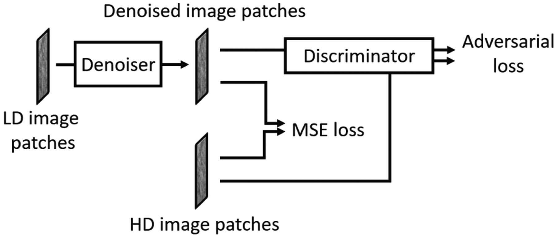
The framework of the denoising DCNN with adversarial training (DNGAN).

2). Training loss function

The training loss function is composed of the MSE loss L_MSE and the adversarial loss L_adv

$$\underset{G}{\text{argmin}}{L}_{\text{MSE}}(G)+{\lambda }_{\text{adv}}\cdot L_{\text{adv}}(G)$$ (1)

where G denotes the denoiser, λ_adv is a tuning parameter controlling the weighting between the MSE loss, which contributes to image smoothness, and the adversarial loss, which contributes to preserving high frequency image textures.

The MSE loss compares the pixel-wise difference between the denoised image patches and the corresponding HD target image patches x_target as follows

$$L_{\text{MSE}}(G)={\mathbb{E}}_{\left(x_{\text{noisy }},x_{\text{target }}\right)}\left[\frac{1}{N_{\text{pixel }}}{\Vert G\left(x_{\text{noisy }}\right)-x_{\text{target }}\Vert }^2\right]$$ (2)

where x_noisy is the LD noisy input patch, N_pixel is the number of pixels in an image patch.

We implemented the adversarial loss as the WGAN with gradient penalty [31]. Section S-II of the Supplementary Materials summarizes the key idea behind the derivation of the adversarial loss. The Wasserstein distance (WD) is estimated as suggested in [30]

$${\widehat{d}}_G(D):={\mathbb{E}}_{x_{\text{target }}}\left[D\left(x_{\text{target }}\right)\right]-{\mathbb{E}}_{x_{\text{noisy }}}\left[D\left(G\left(x_{\text{noisy }}\right)\right)\right]$$ (3)

where D is the discriminator, or a critic, whose output is a similarity score that assesses whether the input image patch comes from the distribution of the target images. The training loss function for the discriminator is

$$\underset{D}{\text{argmin}}-{\widehat{d}}_G(D)+{\lambda }_D\cdot {\mathbb{E}}_{\overline{x}}\left[{\left(\Vert {\nabla }_{\overline{x}}D(\overline{x})\Vert -1\right)}^2\right]$$ (4)

where $\overline{x}=t\cdot x_{\text{target }}+(1-t)\cdot G\left(x_{\text{noisy }}\right)$ is an interpolated image, t~Unif([0,1]), λ_D is the penalty weight. To promote the denoised images to be perceptually similar to the target images, we maximize the term ${\mathbb{E}}_{x_{\text{noisy }}}\left[D\left(G\left(x_{\text{noisy }}\right)\right)\right]$ in ${\widehat{d}}_G(D)$ when optimizing G, which gives the corresponding adversarial loss of the denoiser training

$$L_{\text{adv}}(G)=-{\mathbb{E}}_{x_{\text{noisy }}}\left[D\left(G\left(x_{\text{noisy }}\right)\right)\right].$$ (5)

3). Fine-tuning with MC patches

For DNGAN training, the DBT images with any kind of breast structures can be used for training, as long as the LD/HD image pairs contain matched structures to be preserved and residual differences to be reduced. In our training set preparation, we extracted non-overlapping patches from the DBT slices using a shifting window. A DBT volume mainly consisted of tissue background and there were very few MCs in a volume. Consequently, the training set was dominated by background patches. To emphasize the MC images so that the denoiser could focus on the MC signals and learn to preserve or enhance them, we investigated the feasibility of a second training stage that fine-tuned the DNGAN only with patches centered at individual MCs.

In the fine-tuning stage, we adopted the training technique of layer freezing [45]. For example, freezing m layers means that layers 1 to m in the denoiser were frozen, and layers (m + 1) to the last layer were active. Our denoiser had a total of 10 layers, so m ≤ 10. Note that the freezing was only applied to the denoiser network. All layers in the discriminator were active during training.

B. Data Sets

We prepared several data sets to investigate the effects of the dose level of the HD training target, the training sample size, and the underlying reconstruction algorithm on the performance of our proposed DNGAN. We also prepared a data set for the aforementioned MC fine-tuning experiment. Table I summarizes the data sets and their use in the experiments.

TABLE I.

A Summary of The Data Sets

Purpose	Name	Phantom type	Recon algorithm	No. of patch pairs	Comments
Training	24mAs/target	Digital	SART	199,850	target = 72mAs, 120mAs, 360mAs, noiseless. For investigating the effect of the dose level of the HD training target.
	MC fine-tuning set	Digital	SART	3,048	Patches centered at individual MCs generated at known locations. For investigating the feasibility of a second fine-tuning stage.
	LD/HD-k	Physical	SART	k × 400,000	k = 20%, 35%, 50%, 65%, 80%, 100%. For investigating the effect of the training sample size.
	LD/HD-Pristina	Physical	Pristina	400,000	For training a matched denoiser when evaluating the generalizability of DNGAN in terms of the reconstruction algorithms.
Validation	24mAs as input, higher dose levels as reference truth	Digital	SART	/	Has ground truth scans simulated at multiple dose levels. Used for NPS comparison.
	LD as input, HD as reference for performance comparison	Physical	SART	/	Has individually marked MCs of three nominal diameters. Used for CNR, FWHM, fit success rate, d’, and visual comparisons.
			Pristina	/	For evaluating the generalizability of DNGAN in terms of the reconstruction algorithms.
Test	Human subject DBTs	/	SART	/	An independent test set. For demonstrating the robustness and the feasibility of applying a denoiser trained with phantom data to human DBTs.

As introduced in Section I, we generated two types of data, namely the digital phantom data and the physical phantom data, for DNGAN training and validation. The digital phantom data provided a wide range of x-ray exposures including noiseless images for the study of the effect of the dose level of the HD training target. We also used the digital data to generate the MC fine-tuning set because the coordinates of the simulated MCs were known exactly. Compared with the digital phantom data, the physical phantom data contained all the imaging degradation factors of a DBT system and were considered to be more realistic, and only physical phantom data imaged with the DBT system could be reconstructed with the manufacturer’s proprietary reconstruction technique. We therefore used the physical phantom data for the other experiments and for study of the transferability of a digital-data-trained DNGAN denoiser to real DBT images acquired from physical phantoms and human subjects.

1). Digital phantom data

We prepared 25 heterogeneous dense (34% glandular volume fraction) 4.5-cm-thick digital phantoms at a voxel resolution of 0.05 mm using the VICTRE breast model [40][41]. We inserted simulated MCs consisting of calcium oxalate in clusters into the digital phantoms. Each cluster had 12 MCs arranged on a 3-by-4 grid parallel to the detector plane with a small offset in the direction perpendicular to the chest wall to avoid in-plane artifacts interfering each other during reconstruction. The MCs had three diameters: 0.150 mm, 0.200 mm, 0.250 mm. We used 24 phantoms for training data preparation and held out one phantom for validation.

Next we configured CatSim [42][43] to model the Pristina DBT system (GE Healthcare) that acquires 9 PVs in 25° scan. Section S-III of the Supplementary Materials provides the detailed description of the CatSim configuration. To simulate LD PVs for the digital phantoms, we set the total x-ray exposure of 9 PVs to 24 mAs in CatSim, which was close to the value from automatic exposure control (AEC) for a 4.5 cm breast for the Pristina system [46]. We reconstructed the DBT volumes at a voxel size of 0.1 mm × 0.1 mm × 1 mm using three iterations of simultaneous algebraic reconstruction technique (SART) [7] with the segmented separable footprint projector [47].

2). Physical phantom data

We used seven 1-cm-thick heterogeneous slabs with 50% glandular/50% adipose breast-tissue-equivalent material to construct the physical phantoms [3][4]. By arranging five slabs in different orders and orientations, we formed nine 5-cm-thick phantoms. Clusters of simulated MCs (glass beads) of three nominal diameters (0.150–0.180 mm, 0.180–0.212 mm, 0.212–0.250 mm) were randomly sandwiched between the slabs. Glass beads are used in some commercial breast phantoms but have lower x-ray attenuation than calcium oxalate specks of the same size. We used eight phantoms for training data preparation and held out one phantom for validation.

Each phantom was scanned twice, one at LD and the other at HD, by a Pristina DBT system under the same compression. The LD scans were acquired with the standard dose (STD) setting, which automatically chose a technique of Rh/Ag 34 kVp. The exposures ranged between 30.4 mAs and 32.6 mAs with a mean of 31.4 mAs for the nine phantoms. We manually set the exposure for the HD scans to Rh/Ag 34 kVp, 125 mAs. The reconstruction parameters were the same as those for the digital phantoms.

We marked the MCs in the SART-reconstructed HD volume of the hold-out validation phantom for denoiser evaluation. There was a total of 236 MCs of size 0.150–0.180 mm, 227 MCs of 0.180–0.212 mm, and 159 MCs of 0.212–0.250 mm.

3). Training set generation

Training sets with different target dose levels:

Using CatSim with the digital phantoms, we prepared HD images over a range of dose levels to study the effect of the dose level of the training target images on the effectiveness of the trained denoiser. Specifically, we simulated the HD DBT scans with 72 mAs (3 × AEC), 120 mAs (5 × AEC), 360 mAs (15 × AEC) and noiseless (∞ × AEC) settings. We paired these HD scans with the 24 mAs scans to form four training sets, referred to as 24mAs/72mAs, 24mAs/120mAs, 24mAs/360mAs and 24mAs/noiseless, respectively. We extracted 199,850 pairs of patches from the 24 pairs of SART-reconstructed DBT volumes of the digital phantoms as the training set for each dose condition.

MC fine-tuning set:

We prepared the training set with patches centered at each MC for fine-tuning using the digital phantom data. There were 1,032 MCs of 0.150 mm, 1,008 MCs of 0.200 mm, 1,008 MCs of 0.250 mm in the 24 digital phantoms, giving a total of 3,048 MC patches in the fine-tuning set.

Training sets with different sample sizes:

The generalizability of a trained DCNN depends on the training sample size [48]. We designed an experiment to study the effect of training sample sizes for the DBT denoising task using the physical phantom data. Specifically, we first extracted 400,000 pairs of patches from the eight physical phantoms to form the pool of training patches. Then we randomly drew 20%, 35%, 50%, 65%, 80% of patches from the pool to simulate five training set sizes in addition to the 100% set. These training sets were referred to as LD/HD-k, where k is the drawing percentage. The subset drawing at each percentage was repeated 10 times with different random seeds. Although the independence among the drawn subsets decreased as k increased, the simulation study would provide some understanding of the trend and variation of the training.

Training set of Pristina-reconstructed images:

The Pristina DBT system has a built-in commercial reconstruction algorithm. We refer to it as Pristina algorithm. To evaluate the generalizability of the DNGAN denoiser in terms of the reconstruction algorithms, we directly deployed the denoiser that was trained with SART-reconstructed images to the Pristina-reconstructed images. We also prepared a training set using Pristina-reconstructed images to train a matched denoiser for comparison. This training set was referred to as LD/HD-Pristina and had 400,000 pairs of patches extracted from the eight training physical phantoms.

Section S-IV of the Supplementary Materials shows two examples of the training patches. For all the training sets, we subtracted the mean from each DBT volume to center its histogram before patch extraction.

4). Human subject DBTs

We used eleven de-identified human subject DBT scans, previously collected for another study with IRB approval, as an independent test set to evaluate the denoising effect on the CNR of MCs and the appearances of breast tissue and cancerous masses in real breasts. They contained biopsy-proven invasive ductal carcinomas (masses) and ductal carcinomas in situ (MC clusters). The images were acquired using a GE prototype GEN2 DBT system. The prototype system acquired 21 PVs in a scan angle of 60°. We used the central 9 PVs that corresponded to a scan angle of 24° to simulate an LD DBT with scan parameters like the Pristina DBT system. The DBTs were reconstructed with SART with the same parameters as described above. 301 MCs were marked in the DBT volumes.

C. Figures of Merit

The structural noise power spectrum (NPS) of a breast image quantifies both the structured noise of the object being imaged and other noise on the imaging chain. It has been shown to have a power-law form for mammograms [49]. We used the NPS to quantify the change of textures and noise in the denoised DBT.

To quantitatively evaluate the MCs in the images, we calculated the contrast-to-noise ratio (CNR) and full width at half maximum (FWHM) by fitting a Gaussian function to each MC. For comparison of the performance of the denoiser at different conditions, we calculated the mean and standard deviation of the CNR and the FWHM over the marked MCs at each speck size on the validation physical phantom. The denoiser inevitably smoothed out some subtle MCs as if they were noise. If an MC was very blurred, the fitting program would fit to the background. We set three criteria to automatically mark the fitting as a failure: if the FWHM was larger than twice of the nominal MC size, or if the fitted Gaussian was off centered by two pixels, or if the fitting error was larger than a threshold. These failed MCs were excluded from the mean CNR or mean FWHM calculations, but the fit success rate was counted for each MC speck size and considered one of the indicators of the denoiser performance.

We also calculated the task-based detectability index (d’) from the nonprewhitening matched filter model observer with eye filter (NPWE) as an image quality metric [50][51]. The NPWE observer performance was shown to correlate well with human observer performance [51]–[55]. In this study, we considered the task of detecting MCs of different nominal sizes in the heterogeneous background of breast phantom DBT.

Section S-V of the Supplementary Materials describes the calculation details of the NPS, CNR, FWHM, and d’.

D. DCNN Training Setup

For the DNGAN training, we randomly initialized all the kernel weights. We set the mini-batch size to 512, and λ_D to 10 as suggested [31]. We set λ_adv = 10⁻² The denoiser and the discriminator were trained alternately, and the discriminator had 3 steps of updates for every step of the denoiser update. The discriminator and the denoiser both used Adam optimizer [56] and shared the same learning rate. The learning rate started with 10⁻³ and dropped by a factor of 0.8 for every 10 epochs. The learning rate started with 10⁻⁴ and dropped by a factor of 0.8 for every 50 epochs in the fine-tuning stage. We selected 300 epochs for stage one training and 1,000 epochs for fine-tuning. The selection of λ_adv is shown in Section III.A below. The other parameters, batch size, learning rate, and the number of epochs, were also chosen experimentally based on the training convergence and efficiency as shown in Section S-VI of the Supplementary Materials. The DCNN model was implemented in Python 2.7 and TensorFlow 1.4.1. The training was run on one Nvidia GTX 1080 Ti GPU.

E. Comparison Method

We included a DBT MBIR algorithm developed in our laboratory that models the detector blur and correlated noise (DBCN) with an edge-preserving regularizer [10] for comparison. The parameters (β = 70, δ = 0.002/mm, 10 iterations) that were chosen in [10] were used for reconstructing the DBTs from the GE prototype system. We adapted the DBCN to the Pristina system by adjusting β to 40.

III. Results

A. Effect of Tuning Parameter λ_adv

To demonstrate the effect of λ_adv in (1), we trained six denoisers using λ_adv = 0, 10⁻³, 10⁻², 10⁻¹, 1, ∞ in the DNGAN. The condition λ_adv = 0 is equivalent to using the MSE loss only, and the condition λ_adv = ∞ is equivalent to using the adversarial loss only for DNGAN training. The training set was 24mAs/noiseless. We used the same random seeds for weight initialization and data batching for all conditions.

Fig. 2(a) and (b) shows the training MSE losses and the WD estimate ${\widehat{d}}_G(D)$ defined in (3) versus training epochs. For small λ_adv (0 and 10⁻³), even though they converged to low training MSE values, they had high WD estimates which means that the denoisers produced images that were perceptually dissimilar to the noiseless targets in the training. Note that the WD estimate ${\widehat{d}}_G(D)$ could be increasing or decreasing versus training epochs because the adversarial training aimed at maximizing it over D and minimizing it over G. Fig. 2(c) shows that the denoised validation digital phantoms of λ_adv = 0 and 10⁻³ had low NPS compared to the ground truth noiseless image. This is evidence that the images were overly smoothed and lost structural details.

Fig. 2.

(a) The training MSE losses and (b) the WD estimates for different λ_adv versus training epochs. (c) The NPS curves of the denoised validation digital phantom volumes for different λ_adv.

For λ_adv = 10⁻², 10⁻¹, 1, ∞, although these conditions had similar WD estimates and NPS, the converged training MSE values monotonically increased as λ_adv increased in Fig. 2(a). Moreover, as shown in Fig. 3, for the MCs in the denoised validation physical phantoms, the FWHM increased and the fit success rate dropped substantially as λ_adv increased beyond 10⁻², indicating the blurring and loss of MC signals. Therefore, when the image smoothness was comparable, we preferred λ_adv = 10⁻² for a smaller training MSE and MC preservation.

Fig. 3.

The CNR, FWHM, fit success rates, and d’ of the MCs in the validation physical phantom for different λ_adv. The error bars represent one standard deviation.

B. Effect of Dose Level of Targets on DNGAN Training

To study the effect of the dose level of the training target images on the effectiveness of the denoiser, we trained the DNGAN using the 24mAs/72mAs, 24mAs/120mAs, 24mAs/360mAs, 24mAs/noiseless sets with λ_adv = 10⁻². We used the same random seeds for weight initialization and data batching for all conditions.

Fig. 4 shows that the NPS of the denoised validation digital phantoms matched the NPS of the corresponding CatSim-simulated ground truth volumes. Fig. 5 shows that the DNGAN achieved higher CNR and d’ for the MCs in the validation physical phantoms when the training targets were acquired with a higher dose. However, as the target dose level increased, the fit success rate decreased for the two smaller MC groups. Fig. 6 shows that if the target dose level was very high, for example, 360 mAs or infinity, the tissue backgrounds of the denoised validation physical phantoms images could be too smooth. The smoothing effect of the 24mAs/noiseless denoiser is further demonstrated in human subject DBTs in Section III.F. We used the 24mAs/120mAs for training the DNGAN in the following studies since its dose ratio was closer to that of the LD/HD physical phantom images from a real scan.

Fig. 4.

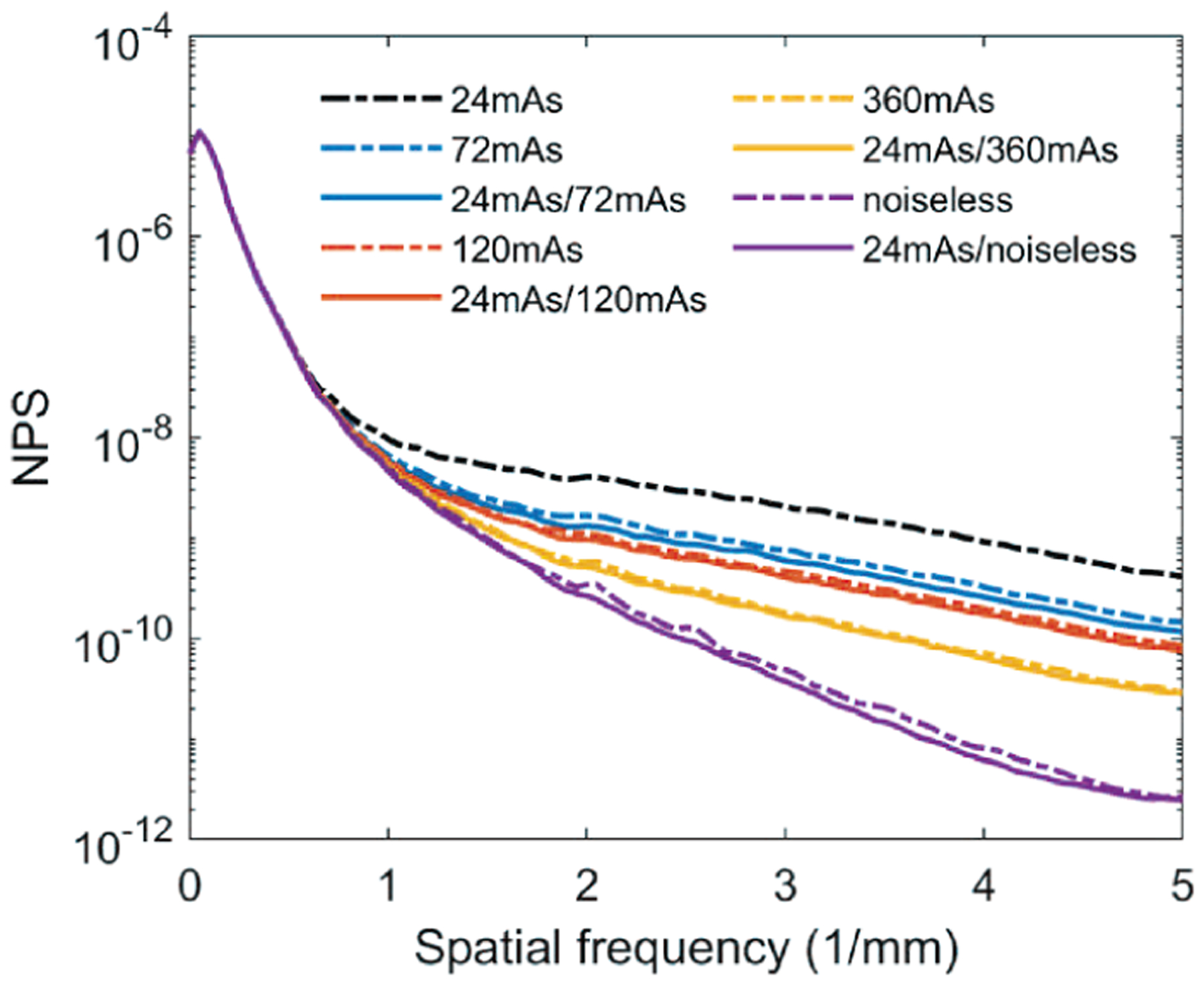
The NPS curves of the validation digital phantom volumes for comparing the dose levels of the training targets. The solid lines are calculated from the volumes by deploying the denoisers to the 24mAs volume. The dashed lines are from the CatSim simulated volumes with the corresponding dose levels.

Fig. 5.

The CNR, FWHM, fit success rates, and d’ of the MCs in the validation physical phantom for the different dose levels of the targets used in the DNGAN training.

Fig. 6.

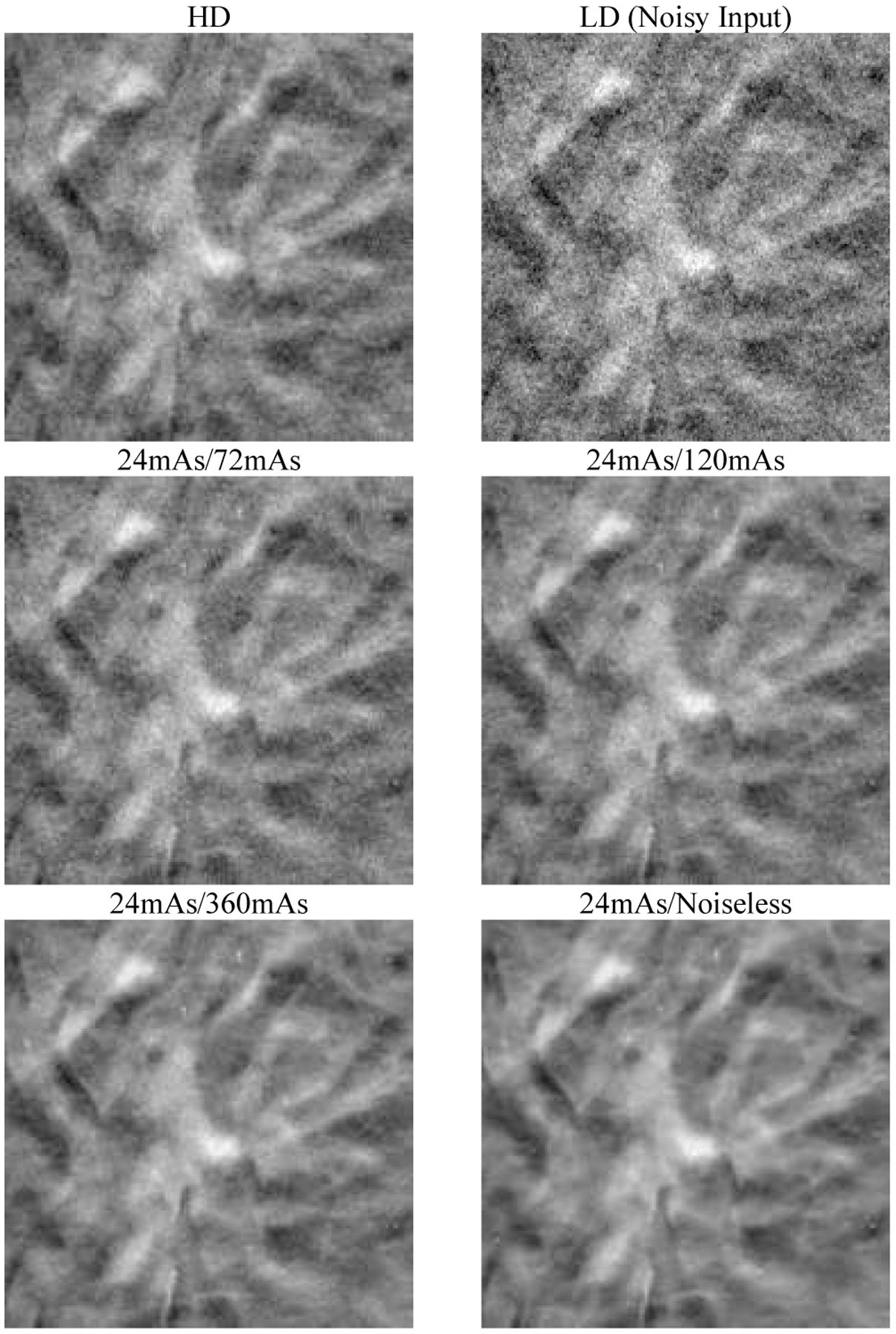
An example 18 mm × 18 mm region in the validation physical phantom for the different dose levels of the targets used in the DNGAN training. The images are displayed with the same window/level settings. The HD scan of the validation physical phantom (34 kVp, 125 mAs) is also shown for reference.

C. Effect of MC Fine-tuning and Layer Freezing

We selected the DNGAN trained with 24mAs/120mAs in Section III.B as the initial model and fine-tuned it using the MC data set. We set the number of frozen layers of the denoiser to 8, 6, 4, 2, 0 while all layers in the discriminator were allowed to be fine-tuned under all conditions. We obtained five fine-tuned denoisers in addition to the base denoiser that was equivalent to freezing 10 layers.

Fig. 7 shows that the fine-tuned denoisers improved the visibility of the subtle MCs in the denoised validation physical phantoms compared to the base denoiser. Fig. 8 shows that the CNR and d’ values increased and the FWHM values decreased as the number of frozen layers decreased, indicating that the MCs became brighter and sharper. The fit success rate also increased for the two smaller MC groups. However, the improvements leveled off when fewer than about 6 layers were frozen. In addition, as seen in the examples in Fig. 7, the fine-tuning not only enhanced the subtle MCs but also some MC-like noise and background structures in the denoised images. The false MCs were obvious and distracting for all the fine-tuned denoisers even though freezing layers mitigated the problem to some extent. The fine-tuning was excluded from further discussions below because we concluded that it was unsuitable for practical use at this point.

Fig. 7.

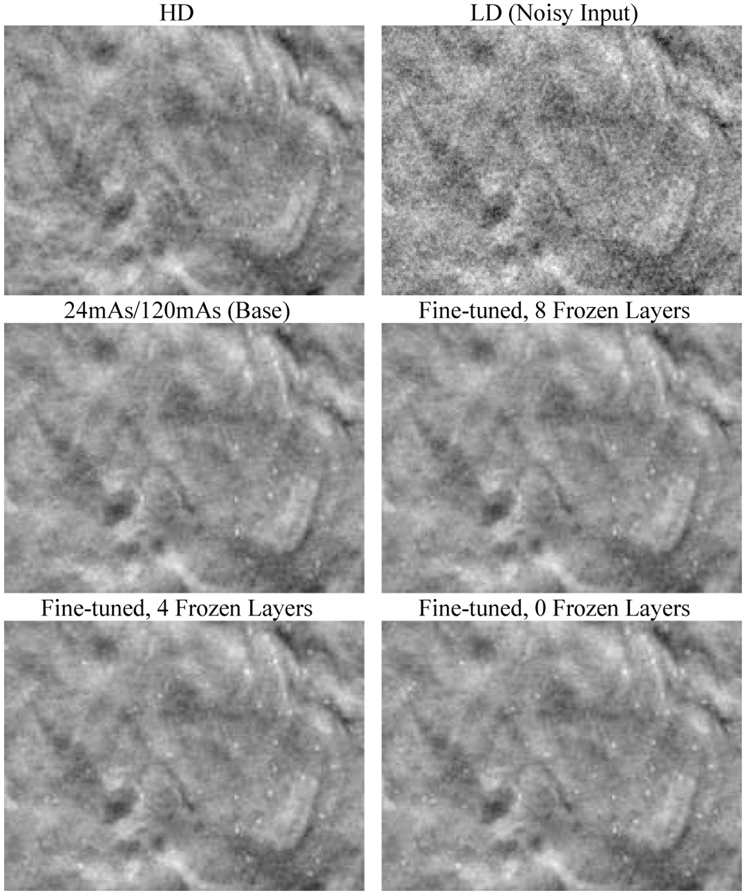
An example 20 mm × 15 mm region in the validation physical phantom showing the effect of fine-tuning and layer freezing. The region contains a background area and a 0.180–0.212 mm MC cluster. The images are displayed with the same window/level settings.

Fig. 8.

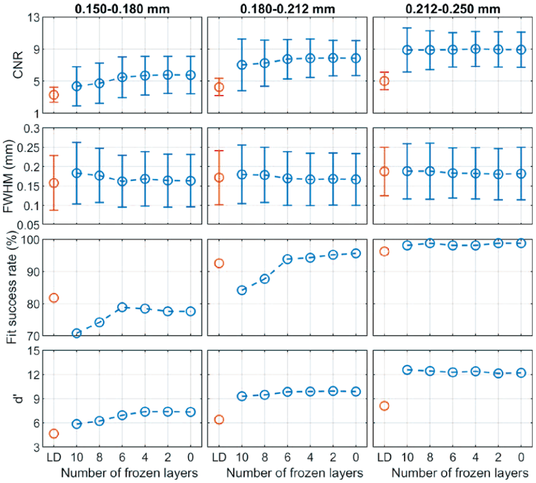
The CNR, FWHM, fit success rates, and d’ of the MCs in the validation physical phantom showing the effect of fine-tuning and layer freezing.

D. Effect of Training Sample Sizes

We trained the DNGAN using the LD/HD-k datasets from the physical phantoms. A different random seed was used for the weight initialization and data batching in each repeated experiment to account for the training randomness. After training, we deployed the denoiser to the validation physical phantom and calculated the mean CNRs for the MCs.

Fig. 9 shows box plots using the 10 repeated experiments versus training data percentage. The general trend was that, when the training sample size increased, the training variation became smaller, and the median CNR increased and became stable. The CNR variations were large at 20% and 35%. This is especially undesirable for DBT because a denoiser with large performance variations can have unpredictable effect on subtle MCs. The large variation can be attributed mainly to the insufficient representation of the imaging characteristics by the small training set and the overfitting of the DCNN to each set of samples. The training randomness from weight initialization and data batching also contributed substantially to the variations, as can be seen from the 100% data point where the training set was the same for all repeated experiments.

Fig. 9.

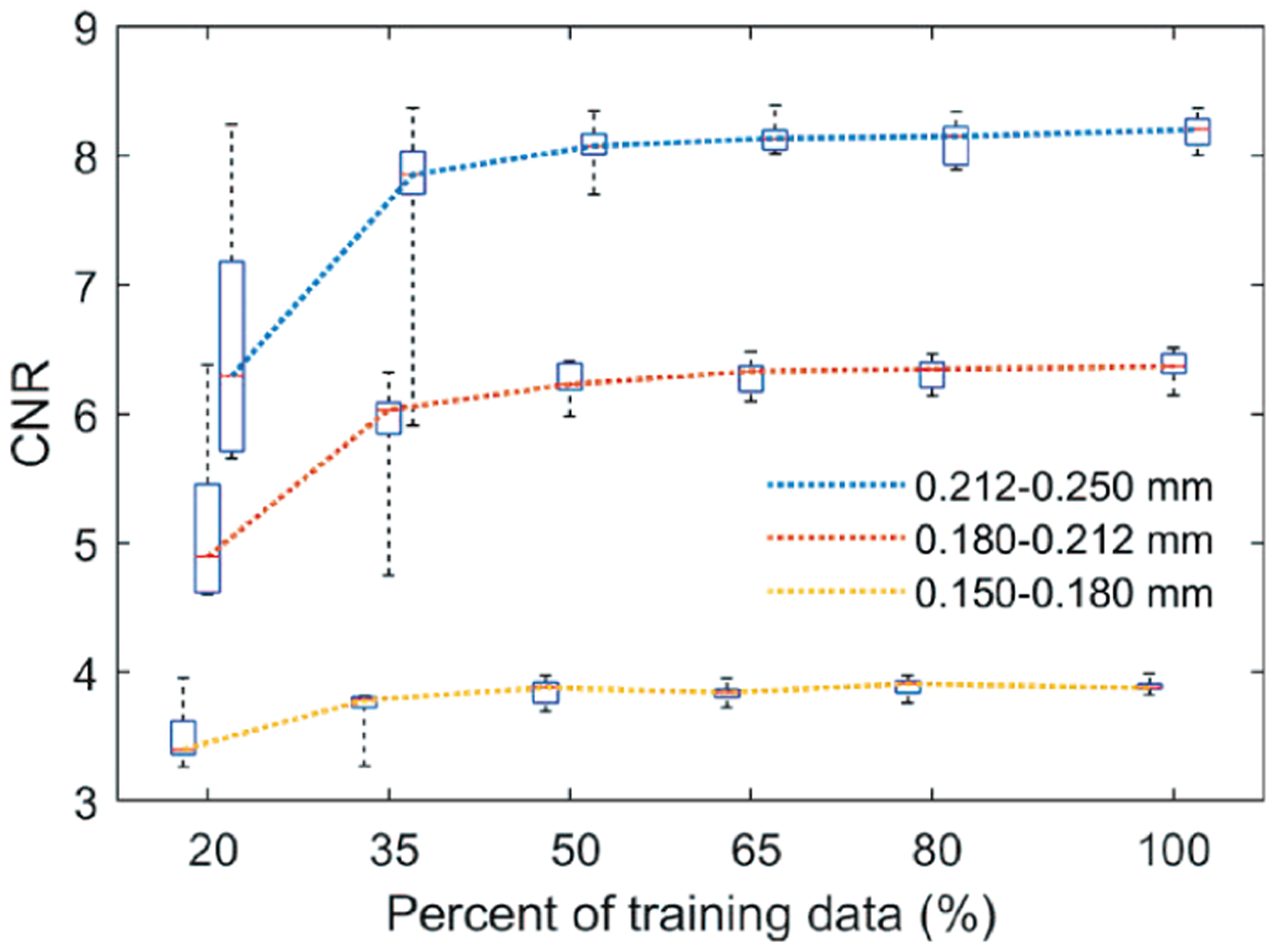
The box plots of the CNRs for different training sample sizes. Each box contains 10 data points. In the box plot, the red bar represents the median; the length of the box equals the interquartile range; the whiskers extend to the minimum and maximum data points. The boxes are slightly shifted horizontally to avoid overlap.

E. Denoising Performance on Validation Physical Phantom

We compared the DNGAN-denoised LD images where the DNGAN was trained with the digital phantom data (24mAs/120mAs) or the physical phantom data (LD/HD-100%), and the LD images reconstructed from the DBCN algorithm. The LD/HD-100% model that was closest to the mean performance among the 10 repeated trainings in Section III.D was used in this comparison.

Fig. 10 shows that the backgrounds in the 24mAs/120mAs and LD/HD-100% denoised validation physical phantoms were perceptually similar to the HD references, with the former being less noisy. Both denoisers improved the CNRs significantly (p < 0.001 for all three MC sizes, two-tailed paired t-test) compared to the LD images, as shown in Fig. 11. Moreover, 24mAs/120mAs had significantly higher CNRs than LD/HD-100% (p < 0.001 for all three MC sizes) with the d’ values showing the same trend. The reason may be that 24mAs/120mAs had a dose ratio of five, while LD/HD-100% had a dose ratio of four and contained scatter and detector noises. A denoiser trained with a higher dose ratio or a less noisy target produced a smoother background, thus larger CNR values. For 24mAs/120mAs and LD/HD-100%, a few more percentages of MCs failed the Gaussian fitting than those in the LD images for the two smaller MC groups, indicating a greater loss of the relative subtle MCs, as also evident in Fig. 10. Fig. 11 shows that the CNRs of MCs in the DBCN images were comparable to those in the 24mAs/120mAs images but were sharper and had higher fit success rates. However, the backgrounds in the DBCN images in Fig. 10 appeared patchier and were noisier than the DNGAN images, which might have contributed to the perceived noise and led to the lower d’ of DBCN than those of 24mAs/120mAs and LD/HD-100% for the two larger MC groups. The CNRs of MCs in the DBCN images were significantly higher than those in the LD images (p < 0.001 for all three MC sizes).

Fig. 10.

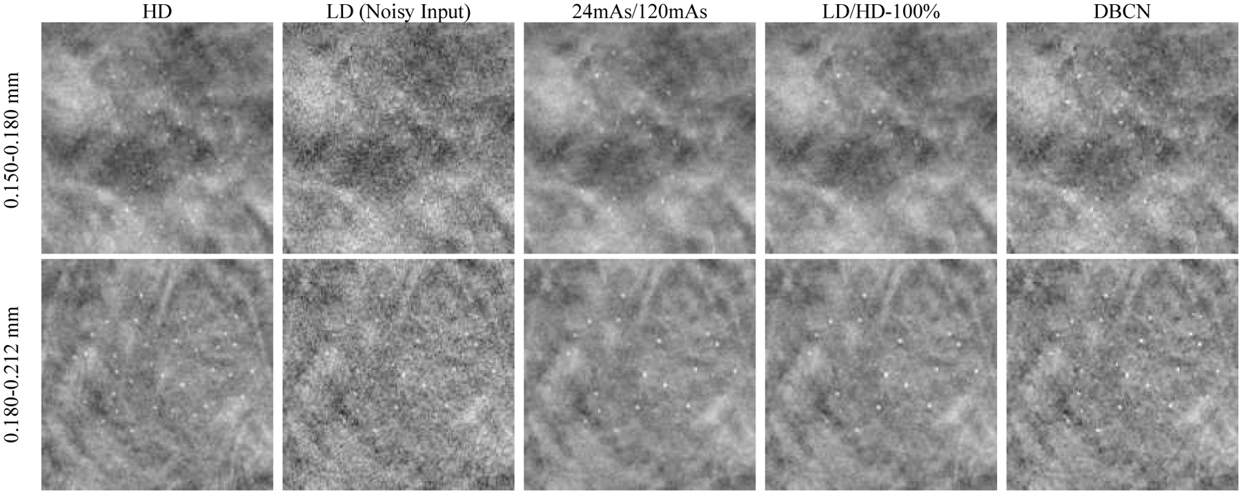
Example MC clusters in the validation physical phantom for comparing the denoising results. All images show a 15 mm × 15 mm region. The images in the same row are displayed with the same window/level settings.

Fig. 11.

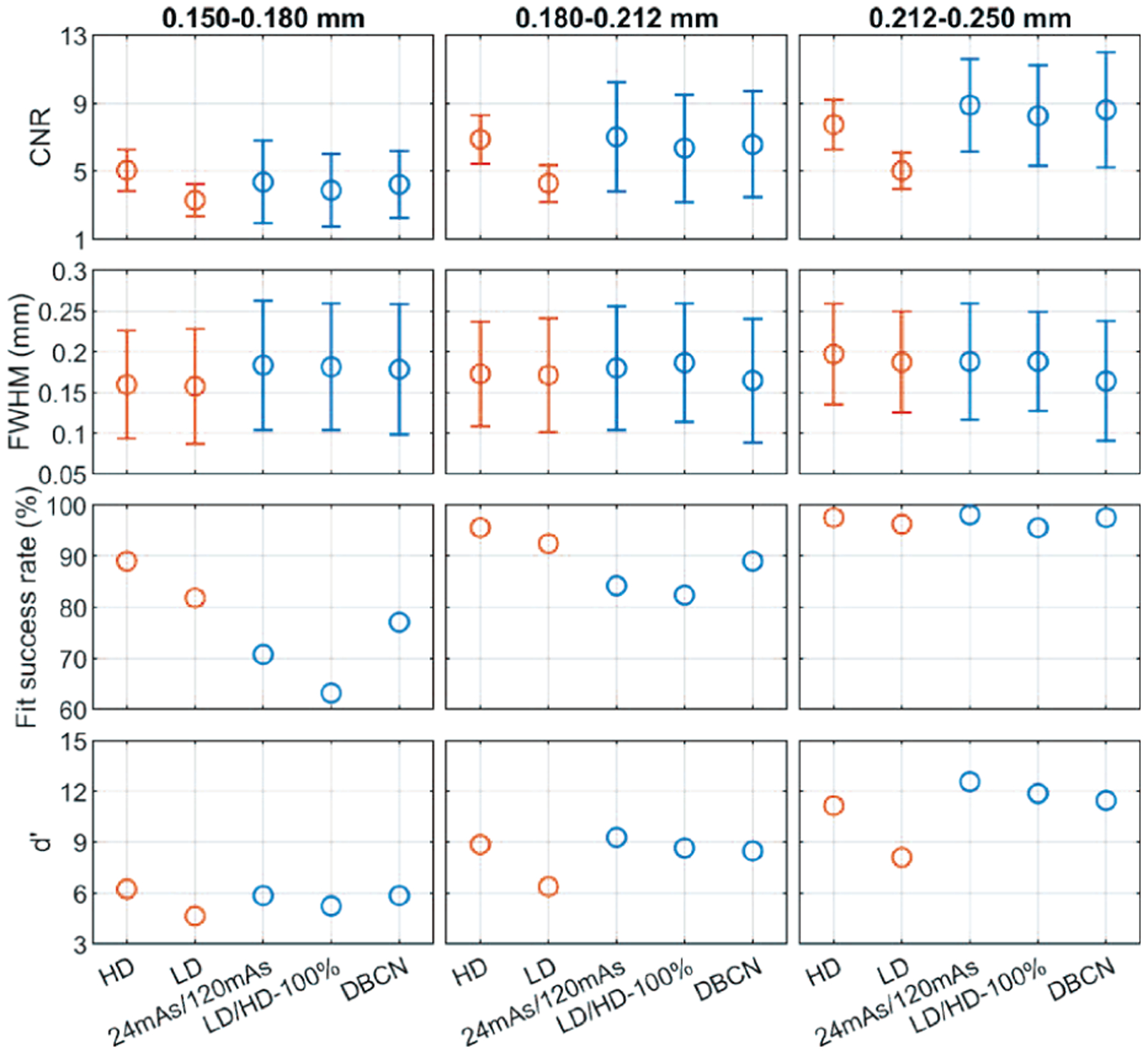
The CNR, FWHM, fit success rates, and d’ of the MCs in the validation physical phantom for comparing the denoising results.

F. Denoising Performance on Human Subject DBTs

We deployed the DNGAN denoisers (24mAs/120mAs and 24mAs/noiseless) to the human subject DBTs for independent testing. Fig. 12 shows that both denoisers and the DBCN were capable of reducing noise and maintaining the margins of the spiculated mass (invasive ductal carcinoma) and improving the conspicuity of the MC cluster (ductal carcinoma in situ). Although the background tissue of the 24mAs/noiseless denoised images was smooth as we discussed in Section III.B, the spiculations were still well preserved. The DBCN images had a patchy and noisier breast parenchyma than the DNGAN denoised images.

Fig. 12.

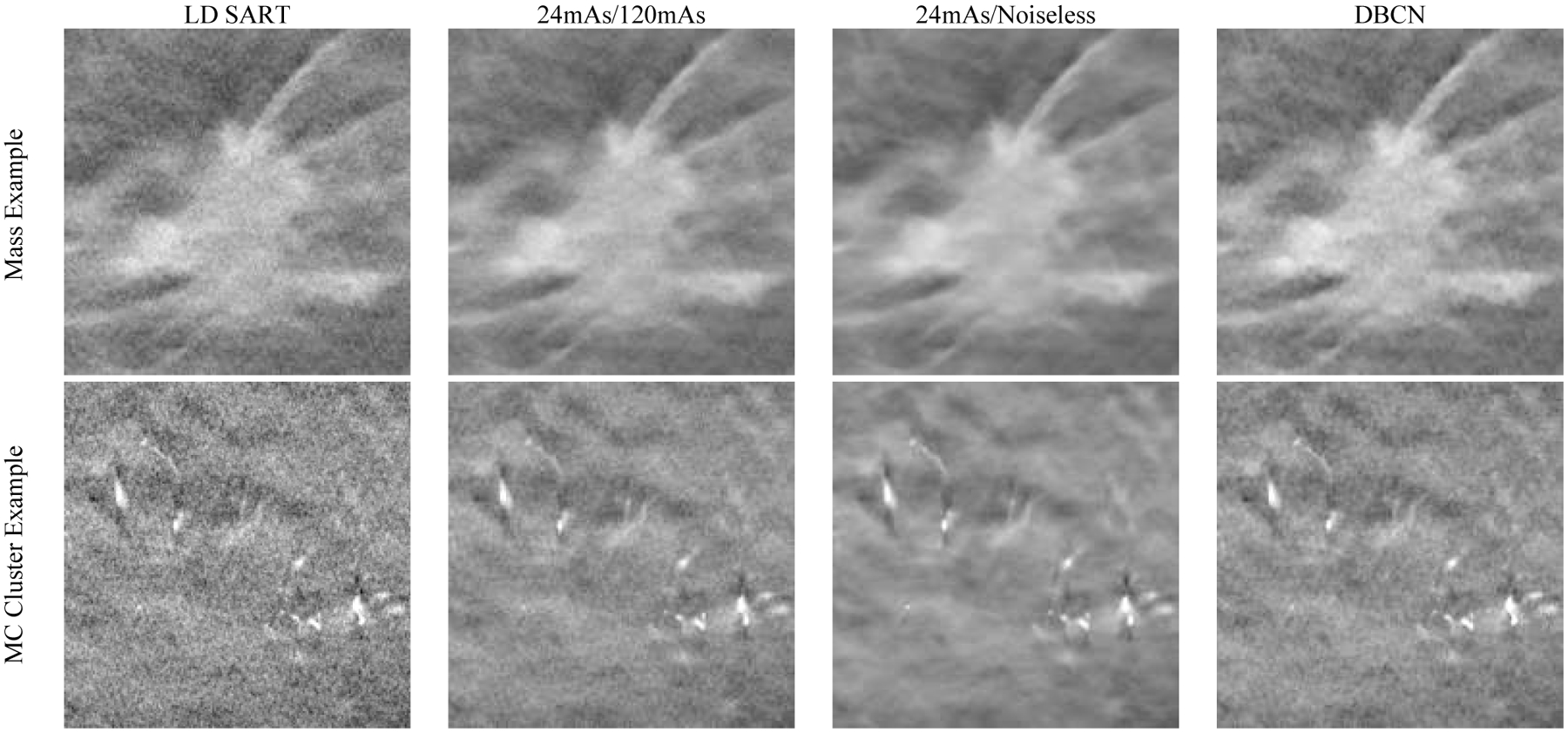
Example images of human subject DBTs with a spiculated mass (invasive ductal carcinoma) and an MC cluster (ductal carcinoma in situ). All images show an 18 mm × 18 mm region. The images in the same row are displayed with the same window/level settings.

Because the MCs in human subjects did not have nominal sizes, instead of comparing the d’ or average CNR values, we generated the CNR scatter plot of individual MCs, as shown in Fig. 13. The CNRs of most MCs were improved after DNGAN denoising. The CNRs of the 24mAs/120mAs denoised images were comparable to those of the DBCN images. The 24mAs/noiseless denoised images had the highest CNRs. However, whether the smooth appearance of the breast parenchyma is acceptable to radiologists and whether it has any effect on diagnosis will warrant future investigations.

Fig. 13.

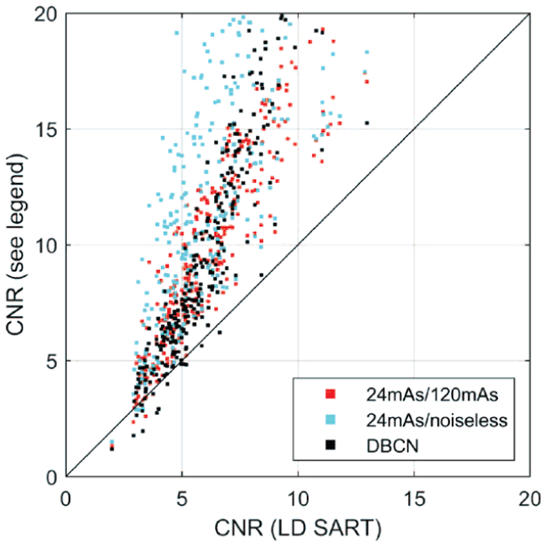
The CNR scatter plot of MCs in the human subject DBTs for the DNGAN denoised images and the DBCN reconstructed images versus the LD SART images.

G. Denoising Pristina-reconstructed Images Using SART Denoiser

To evaluate the generalizability of our DNGAN denoisers in terms of the reconstruction algorithms, we deployed the denoisers trained with SART-reconstructed images to the LD validation physical phantom image that was reconstructed by the Pristina algorithm. Specifically, we selected the 24mAs/120mAs and LD/HD-100% denoisers that were used in Section III.E. We also trained a matched denoiser using the LD/HD-Pristina set.

Fig. 14 shows that the 24mAs/120mAs and LD/HD-100% denoisers worked to certain extent even though they were trained using SART-reconstructed images. The background texture of LD/HD-Pristina denoised images was visually more similar to that of the HD Pristina reference, whereas the 24mAs/120mAs and LD/HD-100% denoisers produced smoother appearance. Fig. 15 shows that all three denoisers reduced the noise and improved the CNRs significantly (p < 0.001 for all three MC sizes) compared to the LD Pristina-reconstructed images. LD/HD-Pristina had higher MC fit success rate and lower FWHM than the other two mismatched denoisers. Fig. 14 and Fig. 15 also included the results of DBCN from Fig. 10 and Fig. 11 to facilitate comparison.

Fig. 14.

Example MC clusters in the Pristina-reconstructed images of the validation physical phantom for comparing the mismatched and matched denoisers. Top row: 0.150–0.180 mm cluster. Bottom row: 0.180–0.212 mm cluster. All images show a 15 mm × 15 mm region. The images in the same row are displayed with the same window/level settings.

Fig. 15.

The CNR, FWHM, fit success rates, and d’ of the MCs in the Pristina-reconstructed images of the validation physical phantom for comparing the mismatched and matched denoisers.

IV. Discussion

The proposed DNGAN enjoys three aspects of robustness. First, the DNGAN trained with phantom data is applicable to human subject DBTs. This avoids the need to train using HD human DBTs, which may be impossible to collect. Second, the DNGAN can be trained with either digital phantom data or physical phantom data. This allows much flexibility in terms of the training data preparation. The digital phantom data have some advantages over the physical phantom data. For example, the software packages for producing the digital phantom data are open-source. It is inexpensive to generate a large set of data once the simulation model is formed, whereas making a large number of realistic physical phantoms is difficult. The high dose level of imaging a physical phantom is also limited by the tube loading of the DBT system. Third, the DNGAN trained with SART-reconstructed images is transferable to denoise other types of images such as Pristina-reconstructed images, although the denoising performance is not as good as that obtained with a denoiser trained with data from matched reconstruction. This makes training DNGAN with in silico data applicable to clinical DBT images for which the reconstruction algorithm is proprietary such as those used in the commercial systems.

For DBT denoising, it seems to be less strict for the training data to be statistically representative of the patient population to achieve generalizability, as we demonstrated that the denoisers trained with digital phantoms were quite effective for physical phantoms and, most importantly, human subject DBTs. One explanation is that the mapping function for DBT denoising is simpler than those for predicting diseases or other clinical tasks. Nevertheless, we only tested the denoiser on a small set of human subject DBTs, so follow-up studies with DBTs of a wide range of properties are needed.

The DNGAN still smoothed out a substantial fraction of the very subtle MCs. We studied the feasibility of a second fine-tuning stage to improve the CNR and d’ of subtle MCs, but the gain was offset by the increased spurious enhancement of noise and background structures (Section III.C). Using our current fine-tuning approach within the DNGAN framework, we have not found a good training condition that could balance between MC enhancement and spurious noise suppression. Further investigations of the training framework to enable the denoiser to distinguish MCs more effectively from noise and selectively enhance the true MCs are warranted.

We compared the image quality obtained from the proposed DNGAN denoising and our DBCN reconstruction. The two approaches represent two different directions to enhance the subtle signals in DBT. The DBCN models the detector blur and correlated noise of the imaging system, which was simplified to essentially a high-frequency-boosting filter on the PVs. To control the high-frequency noise, the DBCN was implemented with an edge-preserving regularizer. However, the reconstructed image quality was sensitive to the choice of the parameters of the regularizer and improper parameters may cause patchy soft tissue texture as discussed by Zheng et al. [10]. In contrast, the DNGAN smoothed the background around the signals to improve their conspicuity, similar to the role of a regularizer, but it also smoothed out some subtle MCs. It would be interesting to incorporate the state-of-the-art deep learning denoiser and the DBCN model into one reconstruction framework [57][58]. Another noteworthy difference between the two methods is that DNGAN is a post-processing approach, whereas DBCN is a reconstruction algorithm. The DNGAN training is relatively flexible and, once fully trained, the DNGAN denoiser is readily deployable to the reconstructed DBT images and potentially applicable to DBT from different reconstruction techniques, as demonstrated in our study. In contrast, DBCN models a given DBT imaging system and requires the raw PVs that may not be stored or accessible in clinical practice. Both approaches have their advantages and disadvantages, and the choice will require future studies to compare the overall cancer detection accuracy and assess the preference of the image appearance by radiologists.

We observed a good correlation between CNR and d’ that we calculated to assess the conspicuity of MCs. Fig. 16 shows a scatter plot of the mean CNR and the corresponding d’ from the results in Section III. The Spearman rank correlation coefficient between CNR and d’ was ρ = 0.96 and the correlation was statistically significant (p < 0.001). This observation suggests that the simple CNR might be a good surrogate for the more sophisticated d’ as an image quality metric of MCs for the task in this study.

Fig. 16.

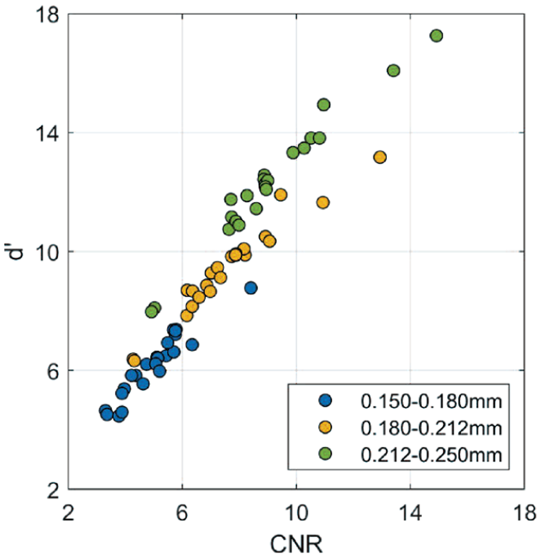
Scatter plot of d’ versus CNR, including all data points from Fig. 3, 5, 8, 11, and 15 for three nominal MC sizes and different conditions.

The figures of merit we used in this study have their limitations. First, CNR was used as an indicator for the conspicuity of individual MCs, but we only calculated CNR at known locations. The clinical usefulness of an image enhancement method has to consider both the true signals and the falsely enhanced noise or structures in an image. Alternative methods, such as computerized detection [59], can be used to study the tradeoff between the increase in detectability of MCs and false positive detection in the future. Second, NPS and d’ are Fourier-based, but the DCNN denoiser is nonlinear and DBT is shift-variant. Third, NPS provides a relative ranking of the noise level of the images, but it does not reflect the visual quality of the soft tissues or masses. To our knowledge, there is no figure of merit available to describe the fine textural appearance of an image or a soft-tissue lesion and correlate it with human visual preference. This makes it difficult to objectively optimize the balance between image smoothness and MC enhancement (Section III.B and Section III.F). The acceptability of the image quality or image appearance for clinical reading will have to be judged by radiologists in human subject DBTs. Reader studies with radiologists can provide more clinically relevant assessments about the pros and cons of each condition but it is impractical to conduct reader studies for many conditions because of the limited availability of radiologists’ time. Reader studies are beyond the scope of this paper.

V. Conclusion

We developed a DNGAN framework based on adversarial training for denoising reconstructed DBT images. A properly weighted combination of an MSE training loss and an adversarial loss was found to be effective for noise reduction and texture preservation. We demonstrated the impacts of the dose level of the training targets and the training sample size on the performance of DBT denoising. We evaluated a fine-tuning stage to further enhance subtle MCs but found that it also enhanced false positives and was unsuitable for practical use. The DNGAN could be trained using in silico data and applied to physical phantom images even from a different reconstruction algorithm. Promising preliminary results were observed in deploying the trained denoiser to a small set of human subject DBTs. Further studies will be conducted to evaluate the effects of the denoiser on the detection of MCs and subtle lesions in DBT by computer vision or human readers.

References

- [1].Dobbins JT, “Tomosynthesis imaging: at a translational crossroads,” Med. Phys, vol. 36, no. 6, pp. 1956–1967, May 2009. [DOI] [PMC free article] [PubMed] [Google Scholar]
- [2].Sechopoulos I, “A review of breast tomosynthesis. Part I. The image acquisition process,” Med. Phys, vol. 40, no. 1, p. 014301, January. 2013. [DOI] [PMC free article] [PubMed] [Google Scholar]
- [3].Chan H-P et al. , “Digital breast tomosynthesis: observer performance of clustered microcalcification detection on breast phantom images acquired with an experimental system using variable scan angles, angular increments, and number of projection views,” Radiology, vol. 273, no. 3, pp. 675–685, 2014. [DOI] [PMC free article] [PubMed] [Google Scholar]
- [4].Goodsitt MM et al. , “Digital breast tomosynthesis: studies of the effects of acquisition geometry on contrast-to-noise ratio and observer preference of low-contrast objects in breast phantom images,” Phys. Med. Biol, vol. 59, no. 19, pp. 5883–5902, October. 2014. [DOI] [PMC free article] [PubMed] [Google Scholar]
- [5].Ludwig J, Mertelmeier T, Kunze H, and Härer W, “A novel approach for filtered backprojection in tomosynthesis based on filter kernels determined by iterative reconstruction techniques,” in Digit. Mammogr. IWDM, 2008, vol. 5116, pp. 612–620. [Google Scholar]
- [6].Liu J et al. , “Radiation dose reduction in digital breast tomosynthesis (DBT) by means of deep-learning-based supervised image processing,” in Proc. SPIE, 2018, p. 105740F. [Google Scholar]
- [7].Zhang Y et al. , “A comparative study of limited-angle cone-beam reconstruction methods for breast tomosynthesis,” Med. Phys, vol. 33, no. 10, pp. 3781–3795, October. 2006. [DOI] [PMC free article] [PubMed] [Google Scholar]
- [8].Das M, Gifford HC, O’Connor JM, and Glick SJ, “Penalized maximum likelihood reconstruction for improved microcalcification detection in breast tomosynthesis,” IEEE Trans. Med. Imaging, vol. 30, no. 4, pp. 904–914, April. 2011. [DOI] [PMC free article] [PubMed] [Google Scholar]
- [9].Xu S, Lu J, Zhou O, and Chen Y, “Statistical iterative reconstruction to improve image quality for digital breast tomosynthesis,” Med. Phys, vol. 42, no. 9, pp. 5377–5390, September. 2015. [DOI] [PMC free article] [PubMed] [Google Scholar]
- [10].Zheng J, Fessler JA, and Chan H-P, “Detector blur and correlated noise modeling for digital breast tomosynthesis reconstruction,” IEEE Trans. Med. Imaging, vol. 37, no. 1, pp. 116–127, January. 2018. [DOI] [PMC free article] [PubMed] [Google Scholar]
- [11].Kim K et al. , “Fully iterative scatter corrected digital breast tomosynthesis using GPU-based fast Monte Carlo simulation and composition ratio update,” Med. Phys, vol. 42, no. 9, pp. 5342–5355, August. 2015. [DOI] [PubMed] [Google Scholar]
- [12].Lu Y, Chan H-P, Wei J, and Hadjiiski LM, “Selective-diffusion regularization for enhancement of microcalcifications in digital breast tomosynthesis reconstruction,” Med. Phys, vol. 37, no. 11, pp. 6003–6014, November. 2010. [DOI] [PMC free article] [PubMed] [Google Scholar]
- [13].Sidky EY, Reiser IS, Nishikawa R, and Pan X, “Image reconstruction in digital breast tomosynthesis by total variation minimization,” in Proc. SPIE, 2007, p. 651027. [Google Scholar]
- [14].Kastanis I et al. , “3D digital breast tomosynthesis using total variation regularization,” in Digit. Mammogr. IWDM, 2008, vol. 5116, pp. 621–627. [Google Scholar]
- [15].Sidky EY et al. , “Enhanced imaging of microcalcifications in digital breast tomosynthesis through improved image-reconstruction algorithms,” Med. Phys, vol. 36, no. 11, pp. 4920–4932, November. 2009. [DOI] [PMC free article] [PubMed] [Google Scholar]
- [16].Zheng J, Fessler JA, and Chan H-P, “Digital breast tomosynthesis reconstruction using spatially weighted non-convex regularization,” in Proc. SPIE, 2016, p. 978369. [Google Scholar]
- [17].Sghaier M, Chouzenoux E, Pesquet J, and Muller S, “A new spatially adaptive TV regularization for digital breast tomosynthesis,” in IEEE Int. Symp. Biomed. Imaging, 2020, pp. 629–633. [Google Scholar]
- [18].Boas FE and Fleischmann D, “CT artifacts: causes and reduction techniques,” Imaging Med, vol. 4, no. 2, pp. 229–240, April. 2012. [Google Scholar]
- [19].Kligerman S et al. , “Detection of pulmonary embolism on computed tomography: improvement using a model-based iterative reconstruction algorithm compared with filtered back projection and iterative reconstruction algorithms,” J. Thorac. Imaging, vol. 30, no. 1, pp. 60–68, January. 2015. [DOI] [PubMed] [Google Scholar]
- [20].Das M, Connolly C, Glick SJ, and Gifford HC, “Effect of postreconstruction filter strength on microcalcification detection at different imaging doses in digital breast tomosynthesis: human and model observer studies,” in Proc. SPIE, 2012, p. 831321. [Google Scholar]
- [21].Abdurahman S, Dennerlein F, Jerebko A, Fieselmann A, and Mertelmeier T, “Optimizing high resolution reconstruction in digital breast tomosynthesis using filtered back projection,” in Digit. Mammogr. IWDM, 2014, vol. 8539, pp. 520–527. [Google Scholar]
- [22].Lu Y, Chan H-P, Wei J, Hadjiiski LM, and Samala RK, “Multiscale bilateral filtering for improving image quality in digital breast tomosynthesis,” Med. Phys, vol. 42, no. 1, pp. 182–195, January. 2015. [DOI] [PMC free article] [PubMed] [Google Scholar]
- [23].Zhang K, Zuo W, Chen Y, Meng D, and Zhang L, “Beyond a Gaussian denoiser: residual learning of deep CNN for image denoising,” IEEE Trans. Image Process, vol. 26, no. 7, pp. 3142–3155, July. 2017. [DOI] [PubMed] [Google Scholar]
- [24].Dong C, Loy CC, He K, and Tang X, “Image super-resolution using deep convolutional networks,” IEEE Trans. Pattern Anal. Mach. Intell, vol. 38, no. 2, pp. 295–307, February. 2016. [DOI] [PubMed] [Google Scholar]
- [25].Kim J, Lee JK, and Lee KM, “Accurate image super-resolution using very deep convolutional networks,” in IEEE Conf. Comput. Vis. Pattern Recognit, 2016, pp. 1646–1654. [Google Scholar]
- [26].Blau Y and Michaeli T, “The perception-distortion tradeoff,” in IEEE Int. Conf. Comput. Vis. Pattern Recognit, 2018, pp. 6228–6237. [Google Scholar]
- [27].Johnson J, Alahi A, and Fei-Fei L, “Perceptual losses for real-time style transfer and super-resolution,” in Eur. Conf. Comput. Vis, 2016, pp. 694–711. [Google Scholar]
- [28].Goodfellow IJ et al. , “Generative adversarial networks,” 2014. [Online]. Available: http://arxiv.org/abs/1406.2661. [Google Scholar]
- [29].Ledig C et al. , “Photo-realistic single image super-resolution using a generative adversarial network,” in IEEE Conf. Comput. Vis. Pattern Recognit, 2017, pp. 105–114. [Google Scholar]
- [30].Arjovsky M, Chintala S, and Bottou L, “Wasserstein GAN,” 26-January-2017. [Online]. Available: http://arxiv.org/abs/1701.07875. [Google Scholar]
- [31].Gulrajani I, Ahmed F, Arjovsky M, Dumoulin V, and Courville A, “Improved training of Wasserstein GANs,” 31-March-2017. [Online]. Available: http://arxiv.org/abs/1704.00028. [Google Scholar]
- [32].Wolterink JM, Leiner T, Viergever MA, and Isgum I, “Generative adversarial networks for noise reduction in low-dose CT,” IEEE Trans. Med. Imaging, vol. 36, no. 12, pp. 2536–2545, December. 2017. [DOI] [PubMed] [Google Scholar]
- [33].Yang Q et al. , “Low-dose CT image denoising using a generative adversarial network with Wasserstein distance and perceptual loss,” IEEE Trans. Med. Imaging, vol. 37, no. 6, pp. 1348–1357, June. 2018. [DOI] [PMC free article] [PubMed] [Google Scholar]
- [34].Hu Z et al. , “Artifact correction in low-dose dental CT imaging using Wasserstein generative adversarial networks,” Med. Phys, vol. 46, no. 4, pp. 1686–1696, April. 2019. [DOI] [PubMed] [Google Scholar]
- [35].Shan H et al. , “3-D convolutional encoder-decoder network for low-dose CT via transfer learning from a 2-D trained network,” IEEE Trans. Med. Imaging, vol. 37, no. 6, pp. 1522–1534, June. 2018. [DOI] [PMC free article] [PubMed] [Google Scholar]
- [36].Shan H et al. , “Competitive performance of a modularized deep neural network compared to commercial algorithms for low-dose CT image reconstruction,” Nat. Mach. Intell, vol. 1, no. 6, pp. 269–276, 2019. [DOI] [PMC free article] [PubMed] [Google Scholar]
- [37].Yang G et al. , “DAGAN: Deep de-aliasing generative adversarial networks for fast compressed sensing MRI reconstruction,” IEEE Trans. Med. Imaging, vol. 37, no. 6, pp. 1310–1321, June. 2018. [DOI] [PubMed] [Google Scholar]
- [38].Mardani M et al. , “Deep generative adversarial neural networks for compressive sensing MRI,” IEEE Trans. Med. Imaging, vol. 38, no. 1, pp. 167–179, January. 2019. [DOI] [PMC free article] [PubMed] [Google Scholar]
- [39].Gao M, Samala RK, Fessler JA, and Chan H-P, “Deep convolutional neural network denoising for digital breast tomosynthesis reconstruction,” in Proc. SPIE, 2020, p. 113120Q. [Google Scholar]
- [40].Badano A et al. , “Evaluation of digital breast tomosynthesis as replacement of full-field digital mammography using an in silico imaging trial,” JAMA Netw. Open, vol. 1, no. 7, p. e185474, November. 2018. [DOI] [PMC free article] [PubMed] [Google Scholar]
- [41].Graff CG, “A new, open-source, multi-modality digital breast phantom,” in Proc. SPIE, 2016, p. 978309. [Google Scholar]
- [42].De Man B et al. , “CatSim: a new Computer Assisted Tomography SIMulation environment,” in Proc. SPIE, 2007, p. 65102G. [Google Scholar]
- [43].De Man B, Pack J, FitzGerald P, and Wu M, “CatSim manual version 6.0,” GE Global Research. 2015. [Google Scholar]
- [44].Isola P, Zhu J-Y, Zhou T, and Efros AA, “Image-to-image translation with conditional adversarial networks,” in IEEE Conf. Comput. Vis. Pattern Recognit, 2017, pp. 5967–5976. [Google Scholar]
- [45].Yosinski J, Clune J, Bengio Y, and Lipson H, “How transferable are features in deep neural networks?,” 2014. [Online]. Available: http://arxiv.org/abs/1411.1792. [Google Scholar]
- [46].“Technical evaluation of GE Healthcare Senographe Pristina digital breast tomosynthesis system,” Public Health England, 2019. [Online]. Available: https://assets.publishing.service.gov.uk/government/uploads/system/uploads/attachment_data/file/771830/GE_Pristina_Tomo.pdf. [Google Scholar]
- [47].Zheng J, Fessler JA, and Chan H-P, “Segmented separable footprint projector for digital breast tomosynthesis and its application for subpixel reconstruction,” Med. Phys, vol. 44, no. 3, pp. 986–1001, March. 2017. [DOI] [PMC free article] [PubMed] [Google Scholar]
- [48].Samala RK et al. , “Breast cancer diagnosis in digital breast tomosynthesis: effects of training sample size on multi-stage transfer learning using deep neural nets,” IEEE Trans. Med. Imaging, vol. 38, no. 3, pp. 686–696, March. 2019. [DOI] [PMC free article] [PubMed] [Google Scholar]
- [49].Burgess AE, “Mammographic structure: data preparation and spatial statistics analysis,” in Proc. SPIE, 1999, p. 3661. [Google Scholar]
- [50].Burgess AE, “Statistically defined backgrounds: performance of a modified nonprewhitening observer model,” J. Opt. Soc. Am. A, vol. 11, no. 4, p. 1237, April. 1994. [DOI] [PubMed] [Google Scholar]
- [51].Loo L-ND, Doi K, and Metz CE, “A comparison of physical image quality indices and observer performance in the radiographic detection of nylon beads,” Phys. Med. Biol, vol. 29, no. 7, pp. 837–856, July. 1984. [DOI] [PubMed] [Google Scholar]
- [52].Burgess AE, Li X, and Abbey CK, “Visual signal detectability with two noise components: anomalous masking effects,” J. Opt. Soc. Am. A, vol. 14, no. 9, p. 2420, September. 1997. [DOI] [PubMed] [Google Scholar]
- [53].Richard S and Siewerdsen JH, “Comparison of model and human observer performance for detection and discrimination tasks using dual-energy x-ray images,” Med. Phys, vol. 35, no. 11, pp. 5043–5053, October. 2008. [DOI] [PMC free article] [PubMed] [Google Scholar]
- [54].Gang GJ et al. , “Analysis of Fourier-domain task-based detectability index in tomosynthesis and cone-beam CT in relation to human observer performance,” Med. Phys, vol. 38, no. 4, pp. 1754–1768, March. 2011. [DOI] [PMC free article] [PubMed] [Google Scholar]
- [55].Christianson O et al. , “An improved index of image quality for task-based performance of CT iterative reconstruction across three commercial implementations,” Radiology, vol. 275, no. 3, pp. 725–734, June. 2015. [DOI] [PubMed] [Google Scholar]
- [56].Kingma D and Ba J, “Adam: A method for stochastic optimization,” 2015. [Online]. Available: http://arxiv.org/abs/1412.6980. [Google Scholar]
- [57].Romano Y, Elad M, and Milanfar P, “The little engine that could: regularization by denoising (RED),” SIAM J. Imaging Sci, vol. 10, no. 4, pp. 1804–1844, January. 2017. [Google Scholar]
- [58].Chan SH, Wang X, and Elgendy OA, “Plug-and-play ADMM for image restoration: fixed-point convergence and applications,” IEEE Trans. Comput. Imaging, vol. 3, no. 1, pp. 84–98, March. 2017. [Google Scholar]
- [59].Samala RK et al. , “Computer-aided detection system for clustered microcalcifications in digital breast tomosynthesis using joint information from volumetric and planar projection images,” Phys. Med. Biol, vol. 60, no. 21, pp. 8457–8479, November. 2015. [DOI] [PMC free article] [PubMed] [Google Scholar]
Associated Data
This section collects any data citations, data availability statements, or supplementary materials included in this article.