

Abstract
Approximately 1.6 million patients in the United States are affected by tricuspid valve regurgitation, which occurs when the tricuspid valve does not close properly to prevent backward blood flow into the right atrium. Despite its critical role in proper cardiac function, the tricuspid valve has received limited research attention compared to the mitral and aortic valves on the left side of the heart. As a result, proper valvular function and the pathologies that may cause dysfunction remain poorly understood. To promote further investigations of the biomechanical behavior and response of the tricuspid valve, this work establishes a parameter-based approach that provides a template for tricuspid valve modeling and simulation. The proposed tricuspid valve parameterization presents a comprehensive description of the leaflets and the complex chordae tendineae for capturing the typical three-cusp structural deformation observed from medical data. This simulation framework develops a practical procedure for modeling tricuspid valves and offers a robust, flexible approach to analyze the performance and effectiveness of various valve configurations using isogeometric analysis. The proposed methods also establish a baseline to examine the tricuspid valve’s structural deformation, perform future investigations of native valve configurations under healthy and disease conditions, and optimize prosthetic valve designs.
Keywords: isogeometric analysis, tricuspid valves, atrioventricular valves, valvular heart disease, parametric modeling, template-based approach
1. Introduction
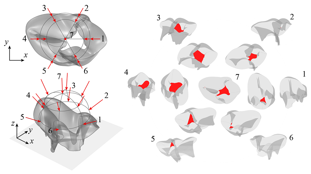
Among the critical anatomical components of the human heart, the four heart valves are the primary structures that regulate unidirectional blood flow through the cardiac system. The atrioventricular valves, with the tricuspid valve (TV) on the right side and the mitral valve on the left side of the heart, regulate the blood flow from the atria to the ventricles. The complex TV anatomy comprises three leaflets: the septal leaflet (SL), anterior leaflet (AL), and posterior leaflet (PL). These leaflets are connected to an annulus at the atrioventricular junction and attached to the papillary muscles in the right ventricle through fibrous cords of tissue known as chordae tendineae (Figure 1). Several valvular pathologies, including stenosis and annular dilation, can inhibit the proper closing of the TV leaflets and lead to various valvular diseases. One such serious insufficiency, known as tricuspid regurgitation, occurs when the improper closure of the TV causes blood to flow back into the atrium during systole [1, 2]. This disease affects approximately 1.6 million Americans and can overload the right ventricle over time as the heart compensates for the reduced cardiac output [3–5].
Figure 1:
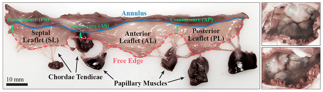
The left image shows an excised porcine tricuspid valve (TV) and the right image shows two intact porcine TVs in the closed configuration. The three leaflets of the TV, the septal leaflet (SL), anterior leaflet (AL), and posterior leaflet (PL), are joined at three commissure locations: the anteroseptal (AS), posteroseptal (PS), and anteroposterior (AP) commissures.
For diseased valves that severely impact proper leaflet closure, common treatment options include either repairing the native valve or replacing it with a prosthetic implant. Despite the high incidence of TV regurgitation and the need for repair and replacement procedures, the TV has received the least research attention among the four heart valves, with the mitral and aortic valves on the left side of the heart being more thoroughly investigated [2, 6, 7]. Through clinical, experimental, and computational approaches, several recent studies have advanced efforts to model and characterize the microstructural properties and mechanical behavior of the TV [2, 7–24]. Many of these studies rely on high-resolution medical image data, such as computed tomography (CT) scans, to reconstruct models of an individual patient’s valve [7, 10]. For computational investigations of the cardiac system, isogeometric analysis (IGA) has recently become a notable approach for modeling heart valve problems [25–41], especially given that spline technologies are frequently utilized for heart valve geometry reconstruction [42–45]. When combined with IGA, spline functions can also be readily employed to analyze complex, patient-specific geometries for vascular modeling problems [46–51]. Recent work has also incorporated spline-based geometries to construct TV models and simulate their function [8, 52] and to develop parametric descriptions that model healthy, diseased, and patient-specific valves [2].
Despite these recent developments, the intrinsically complex geometry and behavior of the atrioventricular valves still present several key challenges in studying the overall function of the TV. While there are numerous methods to construct atrioventricular valves based on medical image data, these approaches rely on high-quality data and are often only suitable for constructing valve-specific geometries based on particular imaging modalities [53, 54]. Valve parameterization, in contrast, offers an effective modeling approach that eliminates the need for specific high-resolution data [28] and enables generative modeling and parametric analysis [55]. Although the utility of parametric modeling has been demonstrated by its effective application to aortic valve simulation [56–58], there are very few existing parametric models for the atrioventricular valves. Additionally, each TV component and its function in the complex valvular system, including the thin structures of the leaflets and the fibrous chordae tendineae, needs to be appropriately described and coupled to replicate the interactions of the entire valve apparatus through simulation. Due to the complexity of these valvular components, there is no existing comprehensive approach to accommodate all of these computational modeling requirements.
To address these challenges, the present work proposes a generalized modeling and analysis framework for the TV. This approach incorporates novel parameterizations, flexible geometric modeling methods, and isogeometric analysis, as outlined in Figure 2, to provide an adaptable framework for simulating the mechanics of the complex valvular surface and chordae tendineae. The developed parametric description generates a simplified TV model that is able to capture the type of structural deformation observed from medical data. When this parameterized model is coupled with IGA, the resulting comprehensive framework provides extensive options for future TV analyses, including examining the performance of healthy and diseased valves and designing and optimizing bioprosthetic valves. This framework also includes proposed methods that allow us to analyze the performance of the TV and extract important quantities of interest, such as the coaptation height and area and the projected regurgitant orifice area, that can be used to evaluate the valve closure and possible regurgitation that may occur.
Figure 2:

Overall schematic of the framework for parameterization, modeling, and isogeometric analysis of tricuspid valves.
The following sections outline the detailed components of this computational framework that produce an adaptable template-based approach that is widely applicable for many TV applications. Section 2 presents the proposed TV parameterization and geometry modeling approaches and the simulation methods that are developed and employed to analyze the TV. These include detailed discussions of the generalized parametric definition, structural formulations, coupling approach, contact algorithm, and material models for the valve leaflets and chordae. In Section 3, the proposed methods and parameterization are applied to the TV. In this section, the developed approaches for evaluating the desired quantities of interest are discussed, and the convergence of the TV modeling and analysis methods is evaluated. A parametric study is also performed to examine the closure behavior of a set of TV cases that are generated and analyzed using the proposed framework. Finally, Section 4 discusses the conclusions of this work and outlines some future applications for this framework.
2. Modeling and simulation methods
2.1. Tricuspid valve parameterization and geometry modeling
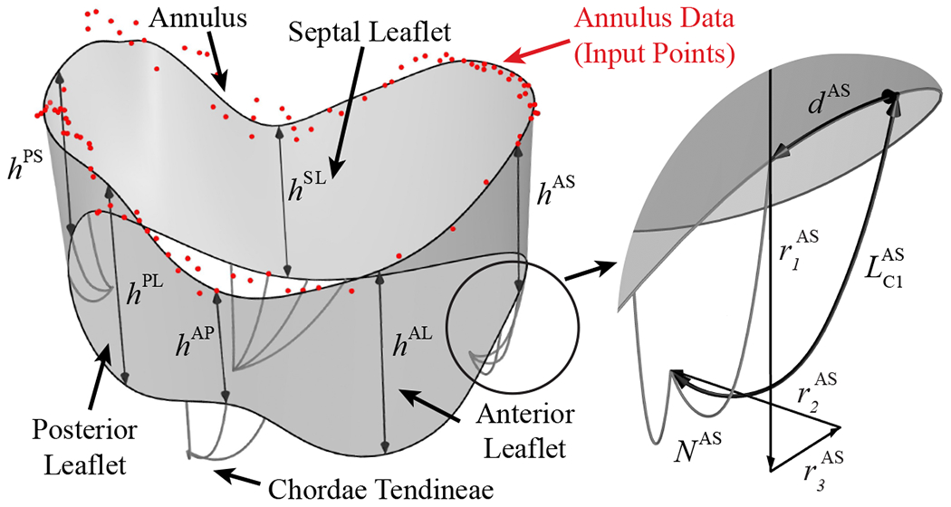
Several imaging modalities are commonly used to capture three-dimensional (3D) medical data from various components of the TV apparatus. Micro-computed tomography (μCT) scans provide high-resolution data that can be used to construct detailed models of the tricuspid and mitral valve geometries [7, 59]; however, this is limited to capturing valves ex vivo or in vitro. For imaging valves in vivo, traditional cardiac CT scans offer a more accessible, lower resolution option to support patient-specific valve reconstruction [10]. 3D transesophageal echocardiography (3D TEE) and cardiac magnetic resonance imaging (MRI) are also commonly used to capture in vivo data from the atrioventricular valves [60–62] and annuli [63, 64]. Considering some of the challenges associated with modeling heart valves directly from medical images, the proposed template-based model has been developed to be data-independent. While the generalized definition of the TV parameters does not require input data from medical images, which is needed for most existing TV modeling approaches, it can also accommodate a variety of medical image resolutions if they are available or necessary for patient-specific modeling. Figure 3 shows the generalized valve parameterization that is proposed and used to construct the template-based model for the TV leaflets and chordae tendineae.
Figure 3:
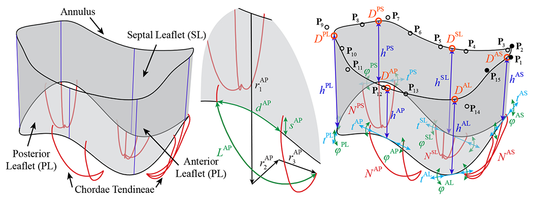
Generalized TV parameterization for the leaflets and chordae tendineae. The model comprises a comprehensive set of parameters, which includes the i control point locations, Pi = (ri, θi, zi). the leaflet and commissure locations, D, and heights, h, the tangential shift, t, and tangential rotation, φ, that control the curvature at the free edge locations, the relative locations of the papillary muscles, r1, r2, and r3. the number of chordae, N, the spacing between chordae, d. the added arc length of the chordae, L, and the offset distance of the outer two chordae in each grouping, s. The superscripts indicate the septal leaflet (SL), anterior leaflet (AL), and posterior leaflet (PL), and the anteroseptal (AS), posteroseptal (PS), and anteroposterior (AP) commissures.
The following subsections present a generalized template for TV parameterization that can be used to model many different valvular arrangements either in vivo or ex vivo. The current work proposes a valvular template that incorporates parameter-based leaflet and chordae modeling approaches to construct B-spline surfaces and curves. This parameter-based model does not directly describe any specihc TV, but accommodates a signihcant number of geometries and configurations. While this generalized parametric valve definition is an independent algorithmic modeling approach that does not require medical data, the versatile model can also incorporate patient-specific information by selecting the individual valve parameters based on input data from medical images. This template-based model takes advantage of the flexibility offered by morphable B-spline geometries and the utility of adaptable parametric modeling approaches to develop a model that can capture many different TV arrangements. The following sections discuss the detailed modeling approaches that are used to construct the TV geometry.
2.1.1. Tricuspid valve leaflet modeling
Within the proposed TV modeling process, the construction approach for the TV leaflet surface begins with generating the annulus curve. In the generalized valve parameterization, the annulus curve is dehned by the 3D cylindrical coordinates, r, θ, and z, of a set of unique control point locations (Figure 4, Step 1). In this work, the control points, Pi are defined by 15 unique point locations that are used to construct the annulus shape as a cubic, periodic B-spline curve with 18 control points, including three overlapping control points (shown with filled markers) to accommodate the cubic periodicity of the surface [65] (Figure 4, Step 2). The total degrees of freedom for the annulus curve can be adjusted to achieve the desired annulus shape. Next, the plane of the annulus curve, which will be used to determine the valve orientation, is defined by fitting a plane to the annulus curve using a least squares fitting algorithm (Figure 4, Step 3). The anteroseptal (AS) commissure location, DAS, is defined at the start and end points of the annulus curve, and the relative positions of the posteroseptal (PS) and the anteroposterior (AP) commissure locations, DPS and DAP, are defined along the one-dimensional (1D) parametric space of the annulus curve (Figure 4, Step 4). Then, the three leaflet locations, DSL, DPL, and DAL, are defined by their relative position between the corresponding commissure locations (Figure 4, Step 5). For notational convenience, note that the superscripts indicating the associated leaflets and commissures are not included in the description of the subsequent TV parameter variables. These relative leaflet positions define the placement of the leaflet and commissure height parameters, h, which determine the offset distance of the free edge at the set positions. Note that the offset direction is defined as the normal direction of the annulus plane, and the offset points define a set of cubic B-spline curves (Figure 4, Step 6) whose end points are then interpolated to construct the bottom edge of the leaflet geometry (Figure 4, Step 7). The open shape of the native TV leaflet is relatively flat, so we construct the leaflet and commissure heights as straight curves, but additional degrees of freedom could also be considered to adjust the curvature of the valve heights.
Figure 4:

Surface construction process for the parameterized TV. The surface model parameters for various steps of the surface construction include the i control point locations. Pi = (ri, θi zi). the leaflet and commissure locations. D, and heights, h, and the tangential shift, t, and tangential rotation, φ, that control the curvature at the free edge locations.
The free edge curvature at each leaflet and commissure location is controlled by the three collinear control points that form a tangent line segment at the leaflet edge. The leaflet shape can be altered by adjusting the length and relative angle of the line segment formed by these three control points, which is accomplished by shifting the outer two points along the tangential direction or by rotating them about the central control point. The tangential shift, t, is a distance factor, defined relative to the length of the annulus curve, that determines the length of the tangent line segment; the tangential rotation, φ, defines the relative rotation of the tangent line segment about the central control point in each set of three collinear control points at the leaflet free edge (Figure 4, Step 8). This final set of cubic B-spline curves describes a bidirectional curve network that is subsequently interpolated to construct the valve leaflets as a Gordon surface [65] (Figure 4, Step 9). This interpolation algorithm utilizes the control point and knot vector information from each individual curve in the network to generate the resulting surface, which, in this work, is a cubic periodic B-spline surface. This Gordon surface has a specific parameterization1 corresponding to the input curves and may be inconsistent in terms of the number of surface control points and knot spans for different cases. Although this parameterization is analysis-suitable, it is not necessarily ideal for the generalized valve analysis and parametric studies in this work, where relatively uniform element sizes and distributions and an equal number of control points for each valve configuration are preferred. To generate a consistent surface parameterization for different configurations, the valve can be reconstructed to obtain the preferred, relatively uniform surface discretization (Figure 4, Step 10). In the present work, we select a consistent, moderate number of control points that will be incorporated in this reconstruction process to obtain a new surface that closely fits the original Gordon surface. Finally, to achieve a model that is sufficiently refined for analysis, several levels of global h-refinement are performed to obtain the refined valve surface (Figure 4, Step 11).
Remark 1. With existing patient or subject information, the TV surface can be constructed using the same valve parameterization approach by selecting the appropriate subset of parameters to match the valve configuration. An example of the TV parameterization including the annulus points from medical data for a porcine valve is shown in Appendix A. A comprehensive table of the TV parameters and the relevant medical imaging modalities from which the parameters could be obtained or estimated is given in Appendix B.
2.1.2. Tricuspid valve chordae tendineae modeling
The constructed valvular surface is connected to a corresponding set of parametrically defined chordae that are intended to reproduce the function of the native chordae. Although the structure of the native chordae is much more complex than the proposed parametric model, similar types of chordae structures have been demonstrated as an effective method to reproduce the behavior and function of the native mitral valve chordae [66]. Several collections of chordae can be employed in the proposed model to accommodate the papillary muscle attachments. The locations of the papillary muscles are first defined by their relative offset from the annulus in the vertical (r1), normal (r2), and tangential (r3) directions (Figure 5, Step 1). The number of chordae, N, is then defined for each group and the spacing between chordae within groupings, d, is defined relative to the corresponding direction in the two-dimensional (2D) parametric space of the B-spline surface (Figure 5, Step 2). This parameterization establishes an adaptive set of chordae whose relative spacing and attachments on the physical 3D surface remains consistent for different input surface parameters. Each papillary location is then attached to the TV surface using a set of parametrically defined planar B-spline curves.2 Instead of a linear chordae connection between the papillary location and the surface attachment, the use of planar curves incorporates an additional arc length, L, which is added in the annular plane direction, that removes the distance limitation between attachment locations (Figure 5, Step 3). The outer two chordae within each grouping can also be connected at an offset distance, s, away from the free edge of the leaflet, which is also defined relative to the corresponding direction in the 2D parametric space of the B-spline surface (Figure 5, Step 4).
Figure 5:

Chordae construction process for the parameterized TV. The model parameters for various steps of the chordae construction include the relative locations of the papillary muscles, r1, r2, and r3, the number of chordae, N, the spacing between chordae, d, the added arc length of the chordae, L, and the offset distance of the outer two chordae in each grouping, s.
Remark 2. To accommodate the papillary muscle attachments and chordae information observed from medical scan data, an appropriate number of chordae groupings can be employed with this model to match the number of papillary muscles and their locations relative to the annulus. The chordae number, lengths, spacing, and offset distances can then be set to approximate available information from the medical data. A comprehensive table of the TV parameters and the relevant medical imaging modalities from which the parameters can be obtained or estimated is given in Appendix B.
2.2. Simulation methods
The TV structure consists of two topologically distinct groups: the leaflet and the chordae tendineae structures. To capture the function of these structures, this work models the leaflets with an IGA shell formulation and the chordae with an IGA cable formulation.3 The shell and cable formulations, as well as the structural coupling between them, are summarized in this section. Such a methodology is capable of accommodating both the leaflets and chordae structures within a single numerical framework.
The formulations defining the structural problems are stated as follows. Find displacement , such that for all test functions :
| (1) |
The semi-linear form B and the linear functional F are defined as
| (2) |
and
| (3) |
where we consider the test function w and the trial function y to be tuples
| (4) |
| (5) |
In the above equations, the superscripts “sh” and “ca” denote quantities associated with the shell and cable subproblem, respectively. The forms Bsh, Bca, Fsh, and Fca encapsulate the non-contact related physics of the shell and cable subproblems. The term δEc (y) models the volume-potential-based contact [52] between the structures, in which δ is a variation (functional derivative) with respect to w and Ec (y) is the contact potential energy. The evaluations of “w” and “y” in this contact term take whatever quantities that are relevant; therefore the formulation can universally handle shell–cable, shell–shell, and cable–cable contacts. The specific forms of the aforementioned terms will be presented in the following sections.
The last term in Eq. (2) formulates the constraints of displacements on the total N points where the chordae end point is attached to the leaflets at . indicates geometric variables in the reference (undeformed) configurations. The constraints are enforced by a penalty method to naturally accommodate the non-conforming discretizations between shells and cables. In general, the value of the penalty parameter βsh-ca can be approximated from the problem properties and the element size through a dimensional analysis. A simpler but effective way, as adopted in this work, is to select a constant value of βsh-ca based on numerical experiments.
2.2.1. Shell structure subproblem
The variational forms of the shell subproblem, Bsh and Fsh, are defined and discretized using a hyperelastic IGA shell formulation [31, 69], which is based on the Kirchhoff–Love thin shell assumption with an arbitrary hyperelastic constitutive model. Higher-order smooth spline functions are used to represent the geometry and displacement in IGA. They provide the H2 regularity of the test and trial spaces as required by the thin shell problem in terms of displacement. In addition, the smooth surface discretization has been reported to improve the performance of contact compared to its finite-element counterpart [70–72]. With the acceleration and velocity of the structures denoted by and , respectively, the semi-discrete form of the nonlinear elasticity problem of leaflet shell structures can be expressed as:
| (6) |
and
| (7) |
where is the shell midsurface with the subscripts 0 and t denoting the reference and current configurations, respectively, is the shell thickness, is the shell mass density in the reference configuration, E is the Green–Lagrange strain tensor, S is the second Piola–Kirchhoff stress tensor, is the through-thickness coordinate, csh is a mass-proportional damping coefficient of the shell, fsh is a prescribed body force, and hsh is the combined effect of the prescribed tractions on the two sides of the shell structure.
In this work, the leaflet soft tissue is assumed to be incompressible and is modeled as a hyperelastic material. Specifically, we calculate S from E in the following way:
| (8) |
where C = 2E + I is the right Cauchy–Green deformation tensor, I is the identity tensor, λp is a Lagrange multiplier for enforcing the material incompressibility, and ψel is an elastic strain energy function. In this work, we adopt an anisotropic (transversely isotropic) Lee–Sacks material model [31]:
| (9) |
where c0, c1, c2, and c3 are material parameters, w ∈ [0, 1] is a parameter that is determined from the material anisotropy, I1 = tr C and I4 = m ⋅ C m are the invariant and pseudo-invariant of C, respectively, and m is a unit vector that defines the collagen fiber direction in the reference configuration.
Native and bioprosthetic valve tissues are typically anisotropic since collagen fibers are oriented in a preferred direction [73]. While material anisotropy can be easily handled by the Kirchhoff–Love shell formulations [31, 74, 75], obtaining collagen fiber orientation data (for instance Jett et al. [76]) is a challenging topic and is outside the focus of this study. Furthermore, the work in Wu et al. [31] suggests that the effect of anisotropy on the large-scale deformation of the leaflets, which determines the geometrical quantities of interest in this paper, such as coaptation or orifice area, is relatively small compared to the sizes of the leaflets. Thus in this paper, we assume w = 1.0, which reduces the Lee–Sacks material model in Eq. (9) to an isotropic model.
While the behavior of soft tissue materials can be accurately modeled as an isotropic Lee–Sacks material, the exponential strain energy description can make the valve modeling quite unstable, especially during the nonlinear iterations. When solving this type of problem with Newton’s method, the intermediate solution predictions can fall into a region of high, unrealistic strain values where the numerical solution can easily diverge for the exponential model. To alleviate this numerical issue, this work proposes an additional hybrid constraint in the elastic strain energy function, ψel, to improve the nonlinear convergence of the shell structures. Under this condition, the absolute value of the (I1 − 3) term is capped at an upper bound, , to stabilize the material model. The new hybrid strain energy function is defined as
| (10) |
where the upper bound should be selected such that it improves the nonlinear convergence of the material model but sets a stress cap that is outside the physical stress levels of the structure throughout the simulation. For simplicity, the incompressibility condition is not directly satisfied within the hybrid regime of the material model when the upper bound constraint is enforced. The selection of an upper bound that is above the physical stress levels ensures that the hybrid constraint is only activated during nonlinear iterations when an intermediate solution prediction exceeds the upper bound, maintaining the incompressibility constraint for solutions in the physical stress regime. Figure 6 shows an example of the effect of this constraint for an equibiaxial tensile test with material parameters of c0 = 10 kPa, c1 = 0.209 kPa, c2 = 9.046, and an upper bound value of .
Figure 6:

Original isotropic Lee–Sacks material model (9) compared to the hybrid model (10) for an equibiaxial tensile test. In this example, c0 = 10 kPa, c1 = 0.209 kPa, c2 = 9.046, and .
2.2.2. Cable structure subproblem
Within the cable subproblem, Bca and Fca are defined using an isogeometric cable formulation that was derived from a 3D continuum, where large-deformation kinematics and the St. Venant–Kirchhoff constitutive law were assumed [77]. The mechanics of the cable are expressed on the 1D center curve, parameterized by a single coordinate ξ1. We denote the reference configuration of the center curve using , on which the points are denoted by . On the deformed configuration , the points are denoted by . The displacement of cable can then be defined as
| (11) |
The covariant and contravariant base vectors for the reference configuration are given by and , respectively, while the base vectors for the deformed configuration are defined without . Considering the small bending stiffness of the chordae tendineae, we omit the bending terms proposed in Raknes et al. [77] and define the cable subproblem as:
| (12) |
and
| (13) |
where is the extensional strain, δε is its variation with respect to wca, is the cable cross-sectional area in the reference configuration, is the cable mass density (per unit volume) in the reference configuration, Eca is the Young’s modulus of the cable structure, cca is a mass-proportional damping coefficient of the cable, fca is a prescribed body force (per unit volume), and hca is a traction (per unit length) prescribed on . Note that the Poisson’s ratio is assumed to be zero in the derivation of this cable formulation.
Although the St. Venant–Kirchhoff material model would typically perform poorly for modeling the large compression of biological soft tissues, it is a more suitable choice for modeling the tensile response of the TV chordae tendineae. The reference configuration of the chordae is reported to have already been stretched beyond the chordae’s soft “pre-transition” regime. The structural simulation of the TV chordae falls into the stiffer “post-transition” regime, in which a more linear stress–strain relation is exhibited. The work of Kunzelman and Cochran [78] reported that the pre-transition stiffness is several orders of magnitude smaller than the post-transition stiffness. Based on this data and following the suggestions of previous studies [79, 80], we neglect the effect of pre-transition stiffness and assume the stress-free reference configuration of the chordae to be the configuration in which tensile strain up to the transition point has been included. With this assumption, the Young’s modulus Eca, as defined in the IGA cable formulation (Eq. (12)), is used as a single parameter to determine the tensile stiffness of the chordae.
2.2.3. Contact formulation
The TV presents multiple contact problems, including leaflet to leaflet, leaflet to chordae, and chordae to chordae contact. A contact formulation in terms of a volume potential permits contact modeling between objects represented by groups of quadrature points and requires no special treatment for contact between arbitrary types of structures (e.g., beams, shells, etc.) with geometric features that would be challenging to handle with traditional contact algorithms. Consider all structural parts to be a single body whose reference configuration is defined as Ω0. We model the contact between two points, x1 and x2, in the deformed configuration as
| (14) |
where and are in Ω0, is the Euclidean ball of radius R around , r12 = x2 − x1 and r12 = ‖r12‖ indicate the distance between two contact points, and is a contact kernel. In this work, the non-penetration condition of objects is strictly enforced to allow objects to simultaneously contact each other without tunneling.4 This requires that the magnitude of the repulsive force as the distance between the two points approaches zero. Considering these requirements, the following force–separation law with an impenetrable core of infinite potential is designed:
| (15) |
where
| (16) |
| (17) |
| (18) |
In the above equations, rmin is the radius within which the kernel goes to infinity, rin is the length scale over which the singular part of the contact kernel acts, rout − rin is the distance over which the polynomial part of the kernel acts, kc is a dimensional constant that determines the magnitude of the repulsive force, p ≥ 4 creates a strong singularity to enforce non-penetrations, and s1 and s2 are constants that ensure the smoothness and continuity of the curve across different segments. A schematic example of can be found in Figure 7, where rcut = rmin + rout is the total distance over which the kernel acts, including the infinite potential. For details on the numerical implementation, we refer the readers to Kamensky et al. [52].
Figure 7:

Illustration of from Eq. (15).
2.2.4. Contact force integration
There are many potential definitions for the contact points that will be used to numerically integrate the contact force. One of the possible options is to employ the same Gaussian quadrature points that are used to integrate the weak forms of the shell and cable subproblems [52], as shown in Figure 8. While this approach is straightforward and can effectively capture the contact force under moderate mesh discretizations, the computational expense of this definition becomes prohibitive with more refined meshes. Another disadvantage of using Gauss points is that the location of the contact points will be inconsistent under global h-refinement, which can make it challenging to obtain consistent solutions.
Figure 8:
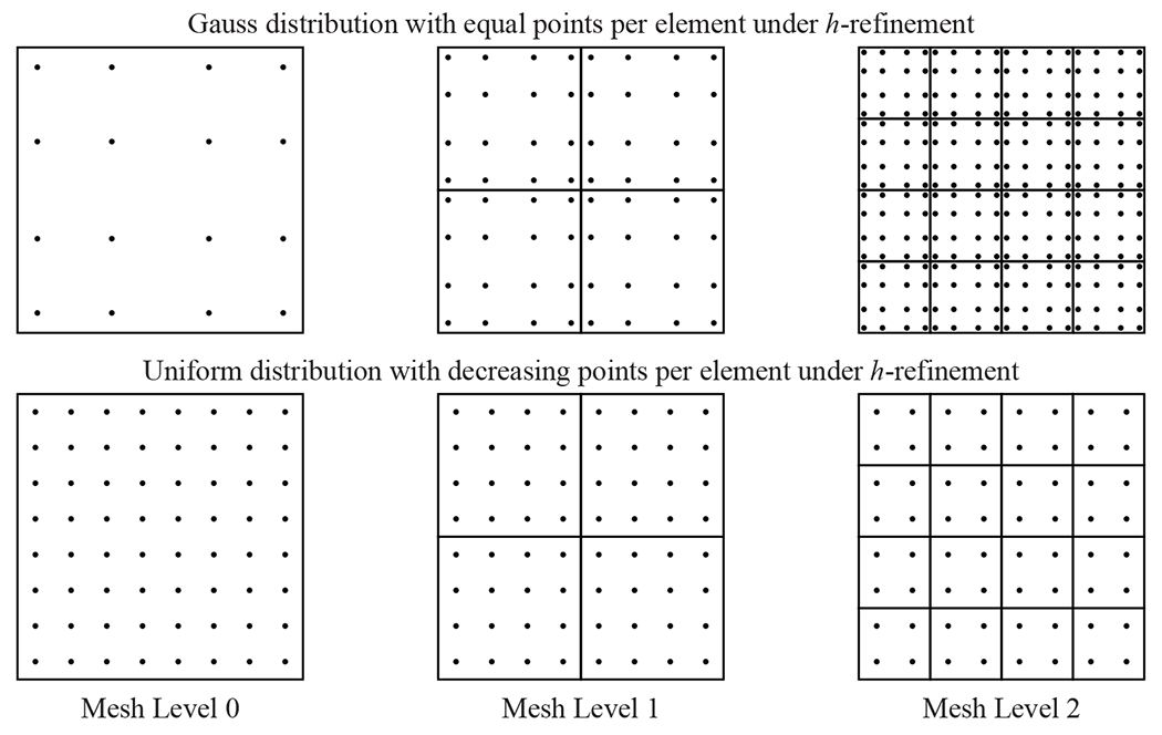
Gauss quadrature and uniform quadrature definitions of the contact points distribution. The Gauss quadrature distribution example is shown for an equal number of points per element at each mesh level, and the uniform quadrature definition is shown for a decreasing number of points per element under h-refinement.
This work proposes an alternative contact point definition that distributes the points so that each one has a uniform influence area across the elements. Under this definition, for a given element with m2 contact points, where m is even, and a parametric domain of {−1, 1} × {−1, 1}, the set of unique uniform contact point locations along one direction of the element domain is defined as , where each point has a uniform weight of . This set of contact quadrature points, which is based on a Newton–Cotes definition [81], is used for the numerical integration of the contact force. For spline-based geometries, this approach also ensures that the contact points will be in the exact same locations under global h-refinement if the number of contact points per element is consistently reduced between mesh levels, as shown in Figure 8.
Remark 3. Note that while it is possible to increase the number of contact points per element for coarser meshes to capture the localized contact forces, this approach will not resolve the local contact behavior if the degrees of freedom in the shell and cable discretizations are not sufficiently refined to represent the physical deformation with contact.
2.2.5. Solution algorithm
The equation system in Eq. (1) is discretized in time using the generalized-α method [82]. However, the singular nature of the contact potential and the highly nonlinear material behavior of the biological soft tissue require special treatments to the standard generalized-α scheme. This work uses a combination of an adaptive time stepping approach and a modified Newton’s method for the nonlinear solution to address these challenges. Specifically, in the modified Newton iteration procedure, the displacement solution field begins with an initial guess and, the solution update from the kth to the (k + 1)th iteration is obtained by , where the scalar αrelax ≤ 1.0 is added due to the standard Newton iteration (with αrelax = 1) being only locally convergent. Specifically, we obtain a tentative prediction of the n + 1 level displacement fields by the current value of αrelax (which is initially set as 1). If the solution fields result in a computationally intractable situation, for example an infinite potential, the αrelax will be reduced to prevent the iterations from rapidly exiting the Newton’s method’s radius of convergence. After this modification, however, the nonlinear iteration may still be prone to stagnation or divergence when the time step size is too large. To remedy this problem, an adaptive time step selection is introduced. The idea is to continuously reduce the time step size by half if it is necessary to maintain the progress of solving. On the other hand, if the nonlinear problem quickly converges in a few iterations, we coarsen the time step size by a factor of two to improve the efficiency. Details of these solution algorithms and their implementations can be found in Kamensky et al. [52].
To further accommodate the nonlinearity of the problem and to improve the robustness of the nonlinear solution procedure, the tangent matrix resulting from the linearization of Eq. (1) is assembled with a larger value of c0. As demonstrated in Kamensky et al. [52], while this approach improves the robustness, it reduces the computational efficiency by requiring more iterations for a converged result. The present work proposes an adaptive procedure that scales with the time step size so that the c0 value in the tangent operator increases automatically when additional robustness is required in the simulation of the valve dynamics, and decreases in the relatively linear regime to improve the solution efficiency. The scaling factor S 0 that is multiplied with c0 is defined as
where n is the time step subdivision level at which the maximum scaling factor is set, with n = 1 for a time step size of Δt = Δtmax/2. In this work, we set n = 4 and .
3. Applications to tricuspid valve modeling and simulation
The proper closure of the TV is a primary concern for TV function and the pathologies that impact valvular dysfunction, such as regurgitation. As a result, the proposed comprehensive framework is intended to provide a flexible, template-based approach to model the TV geometry and mechanics and evaluate the closure performance of such valves. The following sections outline how the proposed framework can be applied to model and simulate different TV configurations.
3.1. Geometric modeling and problem setup
This work focuses on simulating valve closure during the systolic phase of the cardiac cycle. The following demonstrations of the proposed framework and the geometric modeling and simulation approaches incorporate the generalized TV template, including the parameterization and geometry modeling algorithms presented in Section 2.1, to construct the valve geometries. For the TV leaflet properties, the material coefficients for the isotropic Lee–Sacks model are c0 = 10 kPa, c1 = 0.209 kPa, and c2 = 9.046, the mass density is 1.0 g/cm3, and the thickness is 0.0396 cm [52]. An upper bound value of , which sets a stress cap that is outside the physical stress levels of the TV leaflet throughout the simulation, is selected to improve the nonlinear convergence of the material model. For the chordae properties, the Young’s modulus is Eca = 4 × 10⁸ dyn/cm2 = 40 MPa, and the chordae radius is 0.023 cm [52].
To demonstrate the proposed framework, the simulations in this study focus on the closed configuration of the TV. For simplicity, we assume that the annulus curve and papillary muscle locations are in the closed configuration, so we do not consider any papillary muscle or annulus displacement or deformation. The final closed shape of the valve is achieved through simulation by applying a pressure follower load to the ventricular side of the parametrically defined leaflet. The pressure load on the leaflets is linearly increased over the 0 to 0.005 s period from 0 mmHg to the final pressure load of 25 mmHg. This load appropriately represents the typical TV pressure gradients during systole [83].
The energy dissipation to the surrounding blood can be modeled with mass-proportional damping in the leaflets and chordae with damping coefficients csh and cca in Eqs. (6) and (12), respectively. In this paper, the role of the damping is to provide numerical dissipation and ensure that the system is sufficiently damped to reach an equilibrium in the closed configuration, as the focus of this work is to investigate the steady state of valve closure instead of the dynamics. Therefore a value of 5000 s−1 is used for csh and cca, which is larger than the value used in previous dynamic simulations of heart valves [26, 28]. The shell structure subproblem is subject to a pinned boundary condition at the annulus, and the cable subproblem is subject to a pinned boundary condition at the papillary muscle locations.
The B-spline surface and curves that define the leaflet and chordae geometries are used as direct inputs for isogeometric analysis. The pinned boundary condition at the valve annulus is enforced strongly in the discrete model by fixing the first row of control points, and the pinned boundary condition on the chordae is enforced by fixing the chordae control points at the papillary muscle locations. Adaptive time stepping is used with a maximum time step size of Δtmax = 8 × 10⁻⁴ s. The parameters defining the contact kernel are p = 4, kc = 1.0 × 10⁵ cmp−5 s−2g, rcut = 0.04 cm, rmin/rcut = 0.2, and rin/rout = 0.7, which are selected based on the shell thickness, nonlinear convergence behavior, and gap size between surfaces in contact.
3.2. Tricuspid valve quantities of interest
For the TV, there are numerous relevant quantities of interest that can be evaluated to analyze the valve closure and performance and to quantify the effectiveness of different valve configurations. The proposed combined evaluation of the coaptation and the maximum projected regurgitant orifice area (ROA) provides a systematic approach to quantify the valve performance and a suitable method to identify valve closure as well as prolapse and subsequent leaflet flail, which occurs when some portion of the free edge of the leaflet moves through the annulus into the right atrium [84].
3.2.1. Coaptation height and area
The coaptation height is evaluated from the closed configuration of the TV. A 2D slice of the valve is obtained for the deformed geometry from the intersection of a vertical plane (perpendicular to the annulus plane) that cuts through the narrower direction of the TV annulus. Additional intersection planes could also be considered to obtain a more comprehensive view of the coaptation in different regions of the valve. From the resulting intersection curves, the length of the curve segments that are within the contact radius is considered as the coaptation height. The coaptation area can also be evaluated from the 3D deformed valve configuration. This work proposes an approach in which a set of contact area points is used to evaluate the coaptation area. The subset of contact area points within the contact radius threshold are integrated to determine the coaptation area. As will be demonstrated later, although the contact points that are used to simulate the contact force can accurately represent the contact behavior, they are not at a sufficient resolution to evaluate and accurately capture the contact area. The proposed set of higher-resolution contact area points is required to reflect the actual influence area that is within the contact radius threshold. For visualization and quantification, the contact area is evaluated with a set of contact area points at one level higher than the contact points that are used to compute the contact force during the closure simulation. Examples of the coaptation height and area quantities of interest are shown in Figure 9.
Figure 9:
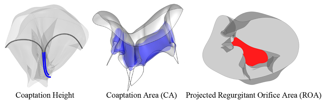
Quantities of interest related to the tricuspid valve closure.
3.2.2. Maximum projected regurgitant orifice area
The final quantity of interest that is evaluated in this work is the maximum projected ROA. In addition to having appropriate coaptation, a properly closed valve geometry that prevents regurgitation should have no areas that close poorly and cause leakage. This work proposes a systematic approach to quantify the geometric area that will result in regurgitation. This quantity of interest provides an effective method for TV evaluation that complements the coaptation quantification to achieve a comprehensive view of the valve closure. To evaluate the extent of leaflet flail and the resulting open regurgitant area, the deformed configuration of the valve is projected onto a plane from a comprehensive set of views. For each direction and projected geometry, the edge of the largest open region is computed and the area of this region is evaluated. The maximum value of the projected orifice area from the entire set of projection directions is selected as the maximum projected ROA. In the case of a valve that closes effectively, the evaluated ROA should be close to zero. An example of the maximum projected ROA is shown in Figure 9, and an example schematic of this process is shown in Figure 10.
Figure 10:
Top and perspective view schematics of the projection directions (left) and resulting projected geometries (right) for an example 13 equally distributed directions from the top view of the valve, with the regurgitant orifice area evaluated from each direction.
3.3. Convergence study
To examine the accuracy and convergence of the computational methods, a mesh convergence study is formulated based on an idealized TV geometry that is generated from the proposed parameterized TV model with a simplified subset of parameters. Projection-based approaches are proposed to achieve consistent convergence for the complex, multi-configuration closure deformation, and the proposed quantities of interest are examined for the simplified geometry. For this convergence study, only one vertical plane at the center of the valve is selected for the evaluation of the coaptation height. As shown in Figure 11, the idealized geometry is constructed with an oval-shaped annulus and has a uniform height of 1.5 cm around the entire valve (total leaflet area of 11.883 cm2). Three pairs of chordae are attached to the annulus at the parametric locations indicated in Figure 11, and the papillary muscle locations are set at 1 cm below the midpoint of the chordae attachments along the leaflet free edge. The surface of the idealized geometry comprises 12 × 4 cubic B-spline elements, and each chordae is modeled as a two-node, linear B-spline element.
Figure 11:

Top, side, and perspective views of the simplified geometry setup for the convergence study. All coordinates and distances are in centimeters (cm).
3.3.1. Approach for problems with multiple solution configurations
For problems with localized buckling behaviors, achieving consistent converged solutions can be challenging when multiple solution configurations can be obtained for the same initial conditions. Because of the complexity of the TV geometry and its closure behavior, multiple closed configurations can easily be induced by different types of perturbations. Throughout the closure simulation, the localized buckling of the valve and added degrees of freedom between meshes can lead to different final configurations for the same initial geometry model (e.g., first row of Figure 12). To ensure that the same unique configuration will be achieved under mesh refinement, a projection-based approach based on the properties of B-splines is proposed to project the deformed configuration of the previous mesh level to the more refined geometry. For a baseline geometry, indicated as mesh level 0 (M0), successive mesh levels (M1, M2, etc.) can be obtained through global h-refinement of the baseline geometry, where mesh level 1 (M1) corresponds to one level of global h-refinement. With the proposed method, successive levels of the projected solution are obtained by projecting the final deformed shape from the previous mesh level (e.g., M1) to the next level (e.g., M2) by refining the deformed shape (e.g., M1 → M2) and evaluating the displacement of the refined nodes. Once the deformation on the refined mesh is determined, where the internal forces are projected from the final configuration of the previous mesh level, the closure simulation is continued with the refined mesh until a new steady-state solution is achieved at the given mesh level. With the proposed approach, consistent converged configurations can be achieved under global h-refinement for problems that have multiple valid solutions.
Figure 12:

Convergence of different closed configurations of the idealized tricuspid valve geometry under global h-refinement with the projection approach, shown from the top view. The first row of deformed configurations is obtained from the beginning of the closure process. Arrows between rows indicate projection from the deformed shape at the given mesh level in the first row. Within each row, the valve configurations at each mesh level are obtained by projecting the final deformed configuration from the previous mesh level and continuing the closure simulation to achieve the corresponding final configuration. Labels A, B, and C indicate the three configurations for mesh level 2.
3.3.2. Mesh convergence study
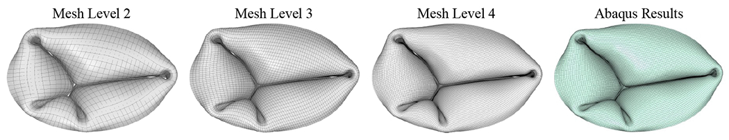
For this study, five different mesh levels of the idealized geometry, as shown in Figure 11, are examined for the different quantities of interest. Mesh level 0, which comprises 24 × 4 cubic B-spline elements, is obtained by performing one level of h-refinement along only the circumferential direction of the baseline geometry. Mesh levels 1–4 are obtained through global h-refinement of mesh level 0. Figure 12 shows the final steady-state configuration at each level of the mesh. The first row of deformed configurations in Figure 12 is obtained from the beginning of the closure process. Each row of the geometry is obtained by projecting the final deformed shape from one mesh level in the first row. Interestingly, although mesh levels 3 and 4 have the same shape, the coarser meshes all deform to different configurations. When the projection approach is used, consistent configurations are achieved for successive levels of global h-refinement.
As shown in Figure 13, we are also able to simulate the same geometry using Abaqus [85] to achieve results that are mesh independent and have a similar closure behavior as configuration A for mesh level 2 (Figure 12). The details of the Abaqus simulation are provided in Appendix C. Figure 14 shows vertical slices for the closed configuration of mesh level 4 compared with the results from mesh levels 2 and 3 and the Abaqus results. The slices are extracted from the vertical planes indicated on the mesh level 4 geometry (Figure 14). The IGA results converge under mesh refinement and are in good agreement with the Abaqus results. The slight discrepancy between the IGA and Abaqus results may arise from the different shell formulations and contact algorithms that are used in the two simulation methods.
Figure 13:
Comparison of Abaqus results with the closed configuration of mesh level 2 (Figure 12, A) and the subsequent closed configurations at mesh level 3 and 4 using the projection approach.
Figure 14:

Vertical slices for the closed configuration of mesh level 4 are compared with the results from mesh levels 2 and 3 and the Abaqus results. The slices are extracted from the vertical planes indicated on the mesh level 4 geometry, which intersect the oval-shaped annulus curve at its minimum x-coordinate, where y = 0, and at x = 0.96 (based on the coordinates in Figure 11).
Figure 15 shows the convergence study for the number of contact area points that are required to evaluate the converged coaptation area quantity of interest. At mesh level 2, the evaluated coaptation area converges with 64 contact area points per element (8 × 8 points). This level of contact area points is selected for the following evaluation of the coaptation area results for each projected mesh level, with the same total number of contact points being used to evaluate the coaptation area at each mesh level. For each configuration, as shown in Figure 16, converged results for the coaptation height and area are obtained under global h-refinement.
Figure 15:

Convergence of the coaptation area under refinement of the contact area evaluation points. Results are shown for each of the three configurations of mesh level 2 in Figure 12, which are indicated as A (solution without mesh projection), B (solution projection from mesh level 1), and C (solution projection from mesh level 0).
Figure 16:

Converged coaptation heights and areas for the solution projected geometries from the configurations at different levels of the mesh.
3.3.3. Solution convergence history
The singular nature of the contact potential and the highly nonlinear material behavior of the biological soft tissue require specific modifications to the solution algorithm, as described in Section 2.2.5. An example case from the convergence study is selected to demonstrate the effectiveness of the proposed methods. Figure 17 shows the adaptive time step size and number of nonlinear iterations over the history of the simulation for configuration A at mesh level 2, which is simulated without any solution projection from the previous mesh level. The results indicate that the adaptive subdivision of the time step size is triggered when the initial contact occurs. At this point in the simulation, additional nonlinear iterations are needed to address the nonlinearity introduced by the numerical contact. However, the combination of the hybrid material model (Eq. (10)) and adaptive scaling factor (Eq. (19)) prevents an excessive increase in the number of iterations. As the simulation approaches steady state, the time step size is coarsened until Δtmax is recovered and only one nonlinear iteration is needed.
Figure 17:

Adaptive time step size and number of nonlinear iterations over the history of the simulation for configuration A at mesh level 2 (Figure 12).
3.4. Tricuspid valve parametric study
The final part of this work is intended to show the flexibility of the proposed framework and how it can be used to simulate many different TV configurations. For this study, 50 cases are sampled from the entire parameter space using Latin hypercube sampling [86]. The input parameters, as shown in Figure 3 and outlined in Section 2.1, for the TV model are constrained within topologically consistent, physically meaningful ranges, shown in Tables 1–3, to ensure that the model will be properly constructed and remain within a suitable range for the size and overall dimensions of a typical porcine valve [19]. The baseline annulus control point values, Ri, Θi, Zi, shown in Table 2, are selected to maintain the appropriate periodic valve topology and the overall saddle shape of a typical TV annulus. Figure 18(a) shows an example TV geometry that is constructed using the median value from the given range of each input parameter. For each case in the parametric study, the periodic valve surface comprises 76 × 16 cubic B-spline elements and 83 × 19 control points, and each chordae curve comprises 4 cubic elements and 7 control points. Figure 18(b) shows the variation in six undeformed valve configurations out of the total set of cases.
Table 1:
TV surface input parameters. The baseline annulus control point values, Ri, θi, Zi, are given in Table 2.
| Surface parameter description | Parameter range |
|---|---|
| Control point radius [cm] | Ri − 0.2 ≤ {ri} ≤ Ri + 0.2 |
| Control point angle [deg] | Θi − 7 ≤ {θi} ≤ Θi + 7 |
| Control point height [cm] | Zi − 0.3 ≤ {zi} ≤ Zi − 0.3 |
| PS commissure location [-] | 0.35 ≤ {DPS} ≤ 0.55 |
| AP commissure location [-] | 0.65 ≤ {DAP} ≤ 0.85 |
| Leaflet locations [-] | 0.4 ≤ {DSL, DPL, DAL} ≤ 0.6 |
| Leaflet heights [cm] | 1.0 ≤ {hSL, hPL, hAL} ≤ 1.7 |
| Commissure heights [cm] | 0.9 ≤ {hAS, hPS, hAP ≤ 1.4 |
| Leaflet edge tangential shift [-] | 0.04 ≤ {tSL, tPL, tAL ≤ 0.1 |
| Commissure edge tangential shift [-] | 0.02 ≤ {tAS, tPS, tAP} ≤ 0.08 |
| Leaflet edge tangential rotation [deg] | −10 ≤ {φSL, φPL, φAL} ≤ 10 |
| Commissure edge tangential rotation [deg] | −10 ≤ {φAS, φPS, φAP} ≤ 10 |
Table 3:
TV chordae tendineae input parameters.
| Chordae parameter description | Parameter range |
|---|---|
| Papillary locations (vertical from annulus) [cm] | |
| Papillary locations (normal to annulus) [cm] | |
| Papillary locations (tangent to annulus) [cm] | |
| Spacing (within each chordae group) [-] | 0.025 ≤ {dSL, dAS, dPS, dAP} ≤ 0.05 |
| Number (per chordae group) [-] | {NSL, NAS, NPS, NAP} ∈ {2,3,4} |
| Arc length (added to straight chordae) [cm] | 0.0 ≤ {LSL, LAS, LPS, LAP} ≤ 0.3 |
| Free edge offsets (outer two chordae in each group) [-] | 0.9 ≤ {sSL, sAS, sPS, sAP} ≤ 1 |
Table 2:
Baseline annulus control point values.
| i | 1 | 2 | 3 | 4 | 5 | 6 | 7 | 8 | 9 | 10 | 11 | 12 | 13 | 14 | 15 |
|---|---|---|---|---|---|---|---|---|---|---|---|---|---|---|---|
| Ri | 1.4 | 1.3 | 1.1 | 0.9 | 0.9 | 1.0 | 1.2 | 1.3 | 1.3 | 1.2 | 1.0 | 0.9 | 0.9 | 1.1 | 1.3 |
| Θi | 0 | 18 | 45 | 72 | 96 | 127 | 145 | 167 | 193 | 215 | 233 | 264 | 288 | 315 | 342 |
| Zi | 0.6 | 0.5 | 0.4 | 0.4 | 0.4 | 0.4 | 0.5 | 0.6 | 0.6 | 0.5 | 0.4 | 0.4 | 0.4 | 0.4 | 0.5 |
Figure 18:

(a) TV geometry with the median values from the parameter ranges in Tables 1–3. (b) Variation in multiple undeformed valve configurations from the set of cases in the parametric study.
The results from the parametric study for the defined quantities of interest are shown in Figures 19 and 20. The filled markers in the plots indicate cases with a low regurgitant orifice area and a relatively high coaptation area. The relative size of the markers is scaled by the size of the maximum ROA. The four cases highlighted in Figures 19 and 20, including two cases with good closure performance and two cases with poor closure performance, are further examined. For these cases, the coaptation area is evaluated for each configuration. In the cases with good closure, as shown in Figure 19, the maximum in-plane principal Green–Lagrange strain (MIPE) on the atrial side of the leaflets is also evaluated. For the cases with poor closure, as shown in Figure 20, the maximum ROA is visualized. For the case with the lower ROA value, case 47, the coaptation height, which is evaluated at the vertical plane that is perpendicular to the annulus plane and intersects the DSL and DAL locations (Figure 4), is also visualized.
Figure 19:

Evaluation of the coaptation area for the set of fifty cases. Filled markers indicate cases with a low regurgitant orifice area and a relatively high coaptation area. The size of the markers indicates the relative size of the maximum ROA. The results from cases 18 and 36 show two valves with good coaptation and closure. Results from cases 9, 26, and 33 are shown in Figure 21.
Figure 20:

Evaluation of the maximum projected ROA for the set of fifty cases. Filled markers indicate cases with a low regurgitant orifice area and a relatively high coaptation area. The size of the markers indicates the relative size of the maximum ROA. The results from cases 15 and 47 show valves with poor closure and some of the highest maximum ROAs. Results from cases 9, 26, and 33 are shown in Figure 21.
Cases 18 and 36 are selected in Figure 19 to show valves with proper closure and large coaptation areas. Both of these cases exhibit the typical three leaflet cusps of the TV, and the uniform coaptation area around the entire geometry indicates that the valve will be properly sealed to prevent regurgitation during closure. Cases 15 and 47 are selected in Figure 20 to show some of the valves that experience significant prolapse and subsequent leaflet flail. In case 15, the coaptation area is actually relatively high because portions of the valve are still in contact, but there is still a large ROA because of the leaflet flail. Similarly in case 47, the coaptation height and area of the valve are quite high, but there is a significant degree of leaflet flail. These two cases both demonstrate the importance of evaluating both the coaptation area and the ROA. These cases can be potentially problematic when evaluating TVs in vivo because many of the current imaging technologies are only able to capture 2D views of the valve. The typical imaging modalities, such as 2D echocardiography, capture 2D image slices of the valve, which can then be used to estimate the coaptation height and some degree of flow regurgitation that may be visible from the images. While these modalities can identify valves that close poorly, it may be more challenging to quantify the extent of regurgitation, and in many cases, evaluating only the coaptation height for a limited number of views may not accurately reflect the full severity of the regurgitation. This is clearly demonstrated in case 47, where the coaptation height and 3D coaptation area and ROA quantities offer differing and potentially misleading evaluations of the closure if only the coaptation height is examined.
Cases 9, 26, and 33 are also highlighted in the plots in Figures 19 and 20. These cases have relatively high coaptation areas, but some aspect of their closure behavior, either possible leaflet flail or a non-negligible level of the ROA, could reduce the performance of these valves and lead to regurgitation. The deformed configurations of cases 9, 26, and 33 are shown in Figure 21 to further examine the closure of these valves. In case 26, the highlighted area shows one leaflet that experienced a small degree of flail. Although this leaflet may still be sufficiently sealed, the condition of this type of minor prolapse and flail in a functioning TV might need to be monitored to ensure that is does not worsen. In cases 9 and 33, the highlighted areas of the valve indicate regions that may not be properly sealed or may have minor leaflet flail and could induce regurgitation. In these cases, the small ROA and possible leaflet flail could induce minor regurgitation in a functioning TV, which might also need to be monitored.
Figure 21:

Results from cases 9, 26, and 33, as indicated in the plots in Figures 19 and 20. These cases have high coaptation areas and relatively low regurgitant orifice areas. In all cases, some aspect of the valve closure behavior might induce some amount of regurgitation. In case 26, one of the leaflets has prolapsed and may experience leaflet flail, and a coaptation height could not be computed for this case due to the leaflet behavior. In cases 9 and 33, the regurgitant orifice areas are low and may have a small degree of leaflet flail, but the relatively small degree of improper closure could still allow blood to leak through the valve.
Overall, this parametric study demonstrates the versatility of the proposed modeling and simulation framework for the TV. It also illustrates the relevance of the proposed quantities of interest when evaluating TV closure for many different valve configurations. The cases presented in this study represent only a small subset of all the possible TV configurations that can be described and evaluated using the proposed template-based modeling and simulation approaches. When simulating TVs, this framework and the recommended metrics offer a comprehensive view, including information from the full 3D valve configuration, through which a more extensive understanding of the TV closure can be realized.
4. Conclusion
In this work, novel approaches for the parameterization, geometric modeling, and simulation of the TV were proposed, including a generalized parametric definition of the valve surface and chordae tendineae, a consistent approach for modeling structural contact, and a robust hybrid material model for the valve leaflets. Additional methods for evaluating the desired quantities of interest, including the coaptation height and area and the regurgitant orifice area, were also developed to quantify the TV closure. The convergence of the TV using these modeling and analysis methods was also evaluated using a proposed projection-based approach to achieve consistent converged results for problems, such as TV closure, that may have multiple solution configurations. Finally, a parametric study was performed to demonstrate the flexibility of these approaches by examining the performance of a set of TV cases that were generated and analyzed using the proposed methods.
Although this template provides a highly versatile approach to TV modeling, there are a number of factors that may constrain certain capabilities of the methods presented in this work. One such limitation is that the material parameters employed for the leaflet and chordae tissues may not capture the physically realistic material behaviors of these valve components. As a result, future studies that use this framework should incorporate more realistic material parameters. Additionally, although an accurate description of the distinct, complex features of the TV may be impeded by quality restrictions of available imaging data, the simplified valve parameterization may produce further geometry limitations that might be reduced if the chordae and valve surface were modeled exactly. This framework could also be updated to accommodate future advances in imaging techniques for the TV, including accurately capturing the chordae configuration as well as the motion of the annulus, chordae, and papillary muscles throughout the cardiac cycle.
Overall, the template-based approach presented in this work provides a novel and powerful computational tool that can be used to model and analyze many TV configurations. As a result, the developments proposed here have many future applications to study the TV and develop an improved understanding of its function. The flexibility of such a template-based model delivers substantial possibilities for modeling patient-specific valves, for either healthy or diseased configurations, and prosthetic device designs. With this framework and the proposed methods, we are able to achieve converged valvular configurations and simulate a variety of different valve designs. In conjunction with additional medical data, including the annulus deformation and deflection and papillary muscle displacement, this template could provide a useful model to simulate the TV dynamics throughout the entire cardiac cycle.
Acknowledgments
This work was supported by the Presbyterian Health Foundation Team Science Grants No. C5122401. C.-H. Lee was partially supported by the American Heart Association Scientist Development Grant (SDG) Award No. 16SDG27760143. M.-C. Hsu was partially supported by the National Heart, Lung, and Blood Institute of the National Institutes of Health under Award Nos. R01HL129077 and R01HL142504. D.W. Laurence was supported in part by the National Science Foundation Graduate Research Fellowship (GRF 2019254233). All this support is gratefully acknowledged. We also thank the Texas Advanced Computing Center (TACC) at The University of Texas at Austin for providing HPC resources that have contributed to the research results reported in this paper. The authors would also like to thank Manoj R. Rajanna at Iowa State University for his assistance in computing the equibiaxial tensile tests for the TV material modeling.
Appendix A. Tricuspid valve parameterization with medical data
With existing patient information, the TV surface can be constructed using the same valve parameterization approach by selecting the appropriate subset of parameters to match the valve configuration. This case provides a demonstration that includes TV annulus data from μCT scans, which can be fit using the cubic periodic B-spline curve with 18 control points to generate the initial annulus shape. The number of control points can also be increased or decreased depending on the number of degrees of freedom that are needed to appropriately fit the annulus data. The relative positions of the three leaflet and commissure locations are translated from the set of medical data onto the fitted annular curve to define the position of the commissure and leaflet heights.
Figure A.1:
TV parameterization for the leaflets and chordae tendineae, including annulus points from medical data for a porcine valve. The subset of valve parameters for this model, including the leaflet and commissure heights, h, the relative locations of the papillary muscles, r1, r2, and r3, the number of chordae, N, the spacing between chordae, d, and the length of the chordae, L, are also shown in the figure.
The same input height parameters determine the offset distances at the relative locations, and the leaflet curvature can also be defined to match the available medical data. The network of curves constructed based on the input annulus information is used to construct the valve leaflets as a Gordon surface. As a demonstration, Figure A.1 shows the valve parameter inputs for the TV surface based on annulus data from a representative porcine TV.
Appendix B. Tricuspid valve parameters
As indicated in the table, many of the input parameters for the TV template can be extracted from medical images. Table B.1 lists all the parameters for the TV framework and the suitable imaging modalities from which they could be extracted. The following abbreviations are used in the table: 3D Transthoracic Echocardiography (TTE), 3D Transesophageal Echocardiography (TEE), Computed Tomography (CT), Cardiac Magnetic Resonance Imaging (MRI).
Table B.1:
TV input parameters. For notational convenience, the surface and chordae parameters have been consolidated, where sets or collections of the same parameter at different TV locations, as indicated in Figure 3 and Sections 2.1.1 and 2.1.2 (e.g., SL, AS, PS, AP), are replaced by (·). The index variable i indicates the number of annulus control points, and the index variable k = 1,2,3 indicates the three coordinates of the papillary locations.
| Surface parameter description | Imaging modality for medical input data |
|---|---|
| Annulus control point coordinates (ri, θi, zi) | TTE [87, 88], TEE [87], CT [10, 87], MRI [64, 89] |
| Commissure locations (DPS, DAP) | TTE [87, 88, 90], TEE [87], CT [10, 87], MRI [64, 89] |
| Leaflet locations (DSL, DPL, DAL) | TTE [90, 91], TEE [91], CT [10] |
| Leaflet and commissure heights (h(⋅)) | TTE [91], TEE [91], CT [10] |
| Free edge tangential shift (t(⋅)) | CT [10] |
| Free edge tangential rotation (φ(⋅)) | CT [10] |
| Chordae parameter description | Imaging modality for medical input data |
| Papillary locations | CT [10] |
| Spacing (within each chordae group) (d(⋅)) | — |
| Number (per chordae group) (N(⋅)) | — |
| Arc length (added to straight chordae) (L(⋅)) | — |
| Free edge offsets (s(⋅)) | — |
Appendix C. Abaqus model and simulation
A finite element simulation of the idealized TV geometry described in Section 3.3 was performed using Abaqus [85] to verify the IGA-based predictions (Figure 13). The leaflet surface was discretized with 18,960 four-node general-purpose finite-strain shell elements (S4), while each chordae was modeled using one 3D truss element (T3D2). The Abaqus VUMAT user-material subroutine was employed for the hybrid material model described in Eq. (10) for the leaflets and the St. Venant–Kirchhoff material for the chordae. The material properties of the leaflets and chordae are identical to those used in the IGA simulations. The frictionless contact of the leaflet surface was modeled using the Abaqus general contact algorithm with a contact penalty stiffness of 5.0 N/cm. Finally, the finite element simulation was performed using Abaqus Explicit dynamics analysis with a maximum time step size of 1 × 10⁻⁶ s to ensure proper convergence.
Footnotes
Publisher's Disclaimer: This is a PDF file of an unedited manuscript that has been accepted for publication. As a service to our customers we are providing this early version of the manuscript. The manuscript will undergo copyediting, typesetting, and review of the resulting proof before it is published in its final form. Please note that during the production process errors may be discovered which could affect the content, and all legal disclaimers that apply to the journal pertain.
In this context, surface parameterization refers to the parametric space and corresponding knot vector definition of the B-spline surface.
Although the realistic chordae tendineae structures comprise thick, fibrous tissues [20], the cable formulation replicates the same function of the chordae in the TV system. To simulate and characterize the internal mechanics of the chordae, the realistic structures could be more comprehensively modeled using solid elements [22].
Specific discussion on the selection of the contact potential and related discussion on the prevention of tunneling can be found in Kamensky et al. [52, Section 2.1].
Declaration of Interest Statement
The authors declare no conflicts of interest.
References
- [1].Hayek E, Gring CN, and Griffin BP. Mitral valve prolapse. The Lancet, 365(9458): 507–518, 2005. [DOI] [PubMed] [Google Scholar]
- [2].Lee C-H, Laurence DW, Ross CJ, Kramer KE, Babu AR, Johnson EL, Hsu M-C, Aggarwal A, Mir A, and Burkhart HM. Mechanics of the tricuspid valve—From clinical diagnosis/treatment, in-vivo and in-vitro investigations, to patient-specific biomechanical modeling. Bioengineering, 6(2):47, 2019. [DOI] [PMC free article] [PubMed] [Google Scholar]
- [3].Stuge O and Liddicoat J. Emerging opportunities for cardiac surgeons within structural heart disease. The Journal of Thoracic and Cardiovascular Surgery, 132(6):1258–1261, 2006. [DOI] [PubMed] [Google Scholar]
- [4].Hinderliter AL, Willis PW, Long WA, Clarke WR, Ralph D, Caldwell EJ, Williams W, Ettinger NA, Hill NS, and Summer WR. Frequency and severity of tricuspid regurgitation determined by doppler echocardiography in primary pulmonary hypertension. American Journal of Cardiology, 91(8):1033–1037, 2003. [DOI] [PubMed] [Google Scholar]
- [5].Badano LP, Ginghina C, Easaw J, Muraru D, Grillo MT, Lancellotti P, Pinamonti B, Coghlan G, Marra MP, and Popescu BA. Right ventricle in pulmonary arterial hypertension: haemodynamics, structural changes, imaging, and proposal of a study protocol aimed to assess remodelling and treatment effects. European Journal of Echocardiography, 11(1): 27–37, 2010. [DOI] [PubMed] [Google Scholar]
- [6].Taramasso M, Pozzoli A, Guidotti A, Nietlispach F, Inderbitzin DT, Benussi S, Alfieri O, and Maisano F. Percutaneous tricuspid valve therapies: the new frontier. European Heart Journal, 38(9):639–647, 2017. [DOI] [PubMed] [Google Scholar]
- [7].Singh-Gryzbon S, Sadri V, Toma M, Pierce EL, Wei ZA, and Yoganathan AP. Development of a computational method for simulating tricuspid valve dynamics. Annals of Biomedical Engineering, 47(6):1422–1434, 2019. [DOI] [PubMed] [Google Scholar]
- [8].Stevanella M, Votta E, Lemma M, Antona C, and Redaelli A. Finite element modelling of the tricuspid valve: A preliminary study. Medical Engineering & Physics, 32(10):1213–1223, 2010. [DOI] [PubMed] [Google Scholar]
- [9].Pouch AM, Aly AH, Lasso A, Nguyen AV, Scanlan AB, McGowan FX, Fichtinger Gabor, Gorman RC, Gorman JH III, Yushkevich PA, and Jolley MA. Image segmentation and modeling of the pediatric tricuspid valve in hypoplastic left heart syndrome. In Pop M and Wright GA, editors, Functional Imaging and Modelling of the Heart, pages 95–105. Springer International Publishing, Cham, 2017. [DOI] [PMC free article] [PubMed] [Google Scholar]
- [10].Kong F, Pham T, Martin C, McKay R, Primiano C, Hashim S, Kodali S, and Sun W. Finite element analysis of tricuspid valve deformation from multi-slice computed tomography images. Annals of Biomedical Engineering, 46(8):1112–1127, 2018. [DOI] [PMC free article] [PubMed] [Google Scholar]
- [11].Rausch MK, Malinowski M, Wilton P, Khaghani A, and Timek TA. Engineering analysis of tricuspid annular dynamics in the beating ovine heart. Annals of Biomedical Engineering, 46(3):443–451, 2018. [DOI] [PubMed] [Google Scholar]
- [12].Jett S, Laurence D, Kunkel R, Babu AR, Kramer K, Baumwart R, Towner R, Wu Y, and Lee C-H. An investigation of the anisotropic mechanical properties and anatomical structure of porcine atrioventricular heart valves. Journal of the Mechanical Behavior of Biomedical Materials, 87:155–171, 2018. [DOI] [PMC free article] [PubMed] [Google Scholar]
- [13].Pokutta-Paskaleva A, Sulejmani F, DelRocini M, and Sun W. Comparative mechanical, morphological, and microstructural characterization of porcine mitral and tricuspid leaflets and chordae tendineae. Acta Biomaterialia, 85:241–252, 2019. [DOI] [PMC free article] [PubMed] [Google Scholar]
- [14].Nguyen AV, Lasso A, Nam HH, Faerber J, Aly AH, Pouch AM, Scanlan AB, McGowan FX, Mercer-Rosa L, Cohen MS, Simpson J, Fichtinger G, and Jolley MA. Dynamic three-dimensional geometry of the tricuspid valve annulus in hypoplastic left heart syndrome with a fontan circulation. Journal of the American Society of Echocardiography, 32(5):655–666, 2019. [DOI] [PMC free article] [PubMed] [Google Scholar]
- [15].Rausch MK, Mathur M, and Meador WD. Biomechanics of the tricuspid annulus: A review of the annulus’ in vivo dynamics with emphasis on ovine data. GAMM-Mitteilungen, 42(3):e201900012, 2019. [DOI] [PMC free article] [PubMed] [Google Scholar]
- [16].Kramer KE, Ross CJ, Laurence DW, Babu AR, Wu Y, Towner RA, Mir A, Burkhart HM, Holzapfel GA, and Lee C-H. An investigation of layer-specific tissue biomechanics of porcine atrioventricular valve anterior leaflets. Acta Biomaterialia, 96:368–384, 2019. [DOI] [PMC free article] [PubMed] [Google Scholar]
- [17].Laurence D, Ross C, Jett S, Johns C, Echols A, Baumwart R, Towner R, Liao J, Bajona P, Wu Y, and Lee C-H. An investigation of regional variations in the biaxial mechanical properties and stress relaxation behaviors of porcine atrioventricular heart valve leaflets. Journal of Biomechanics, 83:16–27, 2019. [DOI] [PMC free article] [PubMed] [Google Scholar]
- [18].Ross CJ, Laurence DW, Richardson J, Babu AR, Evans LE, Beyer EG, Childers RC, Wu Y, Towner RA, Fung K-M, Mir A, Burkhart HM, Holzapfel GA, and Lee C-H. An investigation of the glycosaminoglycan contribution to biaxial mechanical behaviours of porcine atrioventricular heart valve leaflets. Journal of The Royal Society Interface, 16:20190069,2019. [DOI] [PMC free article] [PubMed] [Google Scholar]
- [19].Laurence DW, Johnson EL, Hsu M-C, Baumwart R, Mir A, Burkhart HM, Holzapfel GA, Wu Y, and Lee C-H. A pilot in silico modeling-based study of the pathological effects on the biomechanical function of tricuspid valves. International Journal for Numerical Methods in Biomedical Engineering, 36:e3346, 2020. [DOI] [PMC free article] [PubMed] [Google Scholar]
- [20].Ross CJ, Zheng J, Ma L, Wu Y, and Lee C-H. Mechanics and microstructure of the atrioventricular heart valve chordae tendineae: A review. Bioengineering, 7(1):25, 2020. [DOI] [PMC free article] [PubMed] [Google Scholar]
- [21].Hudson LT, Jett SV, Kramer KE, Laurence DW, Ross CJ, Towner RA, Baumwart R, Lim KM, Mir A, Burkhart HM, Wu Y, and Lee C-H. A pilot study on linking tissue mechanics with load-dependent collagen microstructures in porcine tricuspid valve leaflets. Bioengineering, 7:60, 2020. [DOI] [PMC free article] [PubMed] [Google Scholar]
- [22].Ross CJ, Laurence DW, Hsu M-C, Baumwart R, Zhao YD, Mir A, Burkhart HM, Holzapfel GA, Wu Y, and Lee C-H. Mechanics of porcine heart valves’ strut chordae tendineae investigated as a leaflet–chordae–papillary muscle entity. Annals of Biomedical Engineering, 48(5):1463–1474, 2020. [DOI] [PMC free article] [PubMed] [Google Scholar]
- [23].Ross CJ, Hsu M-C, Baumwart R, Mir A, Burkhart HM, Holzapfel GA, Wu Y, and Lee C-H. Quantification of load-dependent changes in the collagen fiber architecture for the strut chordae tendineae-leaflet insertion of porcine atrioventricular heart valves. Biomechanics and Modeling in Mechanobiology, 20:223–241, 2021. [DOI] [PMC free article] [PubMed] [Google Scholar]
- [24].Ross CJ, Mullins BT, Hillshafer CE, Mir A, Burkhart HM, and Lee C-H. Evaluation of affine fiber kinematics in porcine tricuspid valve leaflets using polarized spatial frequency domain imaging and planar biaxial testing. Journal of Biomechanics, 123:110475, 2021. [DOI] [PMC free article] [PubMed] [Google Scholar]
- [25].Hsu M-C, Kamensky D, Bazilevs Y, Sacks MS, and Hughes TJR. Fluid–structure interaction analysis of bioprosthetic heart valves: significance of arterial wall deformation. Computational Mechanics, 54:1055–1071, 2014. [DOI] [PMC free article] [PubMed] [Google Scholar]
- [26].Kamensky D, Hsu M-C, Schillinger D, Evans JA, Aggarwal A, Bazilevs Y, Sacks MS, and Hughes TJR. An immersogeometric variational framework for fluid–structure interaction: Application to bioprosthetic heart valves. Computer Methods in Applied Mechanics and Engineering, 284:1005–1053, 2015. [DOI] [PMC free article] [PubMed] [Google Scholar]
- [27].Morganti S, Auricchio F, Benson DJ, Gambarin FI, Hartmann S, Hughes TJR, and Reali A. Patient-specific isogeometric structural analysis of aortic valve closure. Computer Methods in Applied Mechanics and Engineering, 284:508–520, 2015. [Google Scholar]
- [28].Hsu M-C, Kamensky D, Xu F, Kiendl J, Wang C, Wu MCH, Mineroff J, Reali A, Bazilevs Y, and Sacks MS. Dynamic and fluid–structure interaction simulations of bioprosthetic heart valves using parametric design with T-splines and Fung-type material models. Computational Mechanics, 55:1211–1225, 2015. [DOI] [PMC free article] [PubMed] [Google Scholar]
- [29].Takizawa K, Tezduyar TE, Terahara T, and Sasaki T. Heart valve flow computation with the integrated Space-Time VMS, Slip Interface, Topology Change and Isogeometric Discretization methods. Computers & Fluids, 158:176–188,2017. [Google Scholar]
- [30].Takizawa K, Tezduyar TE, and Sasaki T. Aorta modeling with the element-based zero-stress state and isogeometric discretization. Computational Mechanics, 59:265–280, 2017. [Google Scholar]
- [31].Wu MCH, Zakerzadeh R, Kamensky D, Kiendl J, Sacks MS, and Hsu M-C. An anisotropic constitutive model for immersogeometric fluid–structure interaction analysis of bioprosthetic heart valves. Journal of Biomechanics, 74:23–31, 2018. [DOI] [PMC free article] [PubMed] [Google Scholar]
- [32].Takizawa K, Tezduyar TE, Uchikawa H, Terahara T, Sasaki T, and Yoshida A. Mesh refinement influence and cardiac-cycle flow periodicity in aorta flow analysis with isogeometric discretization. Computers & Fluids, 179:790–798, 2019. [Google Scholar]
- [33].Balu A, Nallagonda S, Xu F, Krishnamurthy A, Hsu M-C, and Sarkar S. A deep learning framework for design and analysis of surgical bioprosthetic heart valves. Scientific Reports, 9:18560, 2019. [DOI] [PMC free article] [PubMed] [Google Scholar]
- [34].Kamensky D and Bazilevs Y. tIGAr: Automating isogeometric analysis with FEniCS. Computer Methods in Applied Mechanics and Engineering, 344:477–498, 2019. [Google Scholar]
- [35].Wu MCH, Muchowski HM, Johnson EL, Rajanna MR, and Hsu M-C. Immersogeometric fluid–structure interaction modeling and simulation of transcatheter aortic valve replacement. Computer Methods in Applied Mechanics and Engineering, 357:112556, 2019. [DOI] [PMC free article] [PubMed] [Google Scholar]
- [36].Terahara T, Takizawa K, Tezduyar TE, Bazilevs Y, and Hsu M-C. Heart valve isogeometric sequentially-coupled FSI analysis with the space–time topology change method. Computational Mechanics, 65:1167–1187, 2020. [Google Scholar]
- [37].Terahara T, Takizawa K, Tezduyar TE, Tsushima A, and Shiozaki K. Ventricle-valve-aorta flow analysis with the Space–Time Isogeometric Discretization and Topology Change. Computational Mechanics, 65:1343–1363, 2020. [Google Scholar]
- [38].Yu Y, Zhang YJ, Takizawa K, Tezduyar TE, and Sasaki T. Anatomically realistic lumen motion representation in patient-specific space–time isogeometric flow analysis of coronary arteries with time-dependent medical-image data. Computational Mechanics, 65:395–404, 2020. [Google Scholar]
- [39].Johnson EL, Wu MCH, Xu F, Wiese NM, Rajanna MR, Herrema AJ, Ganapathysubramanian B, Hughes TJR, Sacks MS, and Hsu M-C. Thinner biological tissues induce leaflet flutter in aortic heart valve replacements. Proceedings of the National Academy of Sciences, 117:19007–19016, 2020. [DOI] [PMC free article] [PubMed] [Google Scholar]
- [40].Kamensky D. Open-source immersogeometric analysis of fluid–structure interaction using FEniCS and tIGAr. Computers and Mathematics with Applications, 81:634–648, 2021. [DOI] [PMC free article] [PubMed] [Google Scholar]
- [41].Zhang W, Rossini G, Kamensky D, Bui-Thanh T, and Sacks MS. Isogeometric finite element-based simulation of the aortic heart valve: Integration of neural network structural material model and structural tensor fiber architecture representations. International Journal for Numerical Methods in Biomedical Engineering, 37:e3438, 2021. [DOI] [PMC free article] [PubMed] [Google Scholar]
- [42].Aggarwal A, Ferrari G, Joyce E, Daniels MJ, Sainger R, Gorman JH III, Gorman R, and Sacks MS. Architectural trends in the human normal and bicuspid aortic valve leaflet and its relevance to valve disease. Annals of Biomedical Engineering, 42(5):986–998, 2014. [DOI] [PMC free article] [PubMed] [Google Scholar]
- [43].Pouch AM, Tian S, Takebe M, Yuan J, Gorman R Jr, Cheung AT, Wang H, Jackson BM, Gorman III JH, Gorman RC, and Yushkevich PA. Medially constrained deformable modeling for segmentation of branching medial structures: Application to aortic valve segmentation and morphometry. Medical Image Analysis, 26(1):217–231, 2015. [DOI] [PMC free article] [PubMed] [Google Scholar]
- [44].Aggarwal A, Pouch AM, Lai E, Lesicko J, Yushkevich PA, Gorman JH III, Gorman RC, and Sacks MS. In-vivo heterogeneous functional and residual strains in human aortic valve leaflets. Journal of Biomechanics, 49(12):2481–2490, 2016. [DOI] [PMC free article] [PubMed] [Google Scholar]
- [45].Rego BV, Khalighi SH, Drach A, Lai EK, Pouch AM, Gorman RC, Gorman JH III, and Sacks MS. A noninvasive method for the determination of in vivo mitral valve leaflet strains. International Journal for Numerical Methods in Biomedical Engineering, 34 (12):e3142, 2018. [DOI] [PubMed] [Google Scholar]
- [46].Bazilevs Y, Calo VM, Zhang Y, and Hughes TJR. Isogeometric fluid–structure interaction analysis with applications to arterial blood flow. Computational Mechanics, 38:310–322, 2006. [Google Scholar]
- [47].Zhang Y, Bazilevs Y, Goswami S, Bajaj C, and Hughes TJR. Patient-specific vascular NURBS modeling for isogeometric analysis of blood flow. Computer Methods in Applied Mechanics and Engineering, 196:2943–2959, 2007. [DOI] [PMC free article] [PubMed] [Google Scholar]
- [48].Bazilevs Y, Gohean JR, Hughes TJR, Moser RD, and Zhang Y. Patient-specific isogeometric fluid–structure interaction analysis of thoracic aortic blood flow due to implantation of the Jarvik 2000 left ventricular assist device. Computer Methods in Applied Mechanics and Engineering, 198:3534–3550, 2009. [Google Scholar]
- [49].Hossain SS, Zhang Y, Liang X, Hussain F, Ferrari M, Hughes TJR, and Decuzzi P. In silico vascular modeling for personalized nanoparticle delivery. Nanomedicine, 8(3):343–357, 2013. [DOI] [PMC free article] [PubMed] [Google Scholar]
- [50].Hossain SS, Zhang Y, Fu X, Brunner G, Singh J, Hughes TJR, Shah D, and Decuzzi P. Magnetic resonance imaging-based computational modelling of blood flow and nanomedicine deposition in patients with peripheral arterial disease. Journal of The Royal Society Interface, 12(106):20150001, 2015. [DOI] [PMC free article] [PubMed] [Google Scholar]
- [51].Urick B, Sanders TM, Hossain SS, Zhang YJ, and Hughes TJR. Review of patient-specific vascular modeling: template-based isogeometric framework and the case for cad. Archives of Computational Methods in Engineering, 26(2):381–404, 2019. [Google Scholar]
- [52].Kamensky D, Xu F, Lee C-H, Yan J, Bazilevs Y, and Hsu M-C. A contact formulation based on a volumetric potential: Application to isogeometric simulations of atrioventricular valves. Computer Methods in Applied Mechanics and Engineering, 330:522–546, 2018. [DOI] [PMC free article] [PubMed] [Google Scholar]
- [53].Lee C-H, Oomen PJA, Rabbah JP, Yoganathan A, Gorman RC, Gorman JH III, Amini R, and Sacks MS. A high-fidelity and micro-anatomically accurate 3D finite element model for simulations of functional mitral valve. In Ourselin S, Rueckert D, and Smith N, editors, Functional Imaging and Modeling of the Heart, pages 416–424. Springer, Berlin, Heidelberg, 2013. [DOI] [PMC free article] [PubMed] [Google Scholar]
- [54].Khalighi AH, Rego BV, Drach A, Gorman RC, Gorman JH III, and Sacks MS. Towards patient-specific mitral valve surgical simulations. In Sacks MS and Liao J, editors, Advances in Heart Valve Biomechanics: Valvular Physiology, Mechanobiology, and Bioengineering, pages 471–487. Springer International Publishing, Cham, 2018. [Google Scholar]
- [55].Li K and Sun W. Simulated transcatheter aortic valve deformation: A parametric study on the impact of leaflet geometry on valve peak stress. International Journal for Numerical Methods in Biomedical Engineering, 33(3):e02814, 2017. [DOI] [PMC free article] [PubMed] [Google Scholar]
- [56].Labrosse MR, Beller CJ, Robicsek F, and Thubrikar MJ. Geometric modeling of functional trileaflet aortic valves: development and clinical applications. Journal of Biomechanics, 39(14):2665–2672, 2006. [DOI] [PubMed] [Google Scholar]
- [57].Haj-Ali R, Marom G, Zekry SB, Rosenfeld M, and Raanani E. A general threedimensional parametric geometry of the native aortic valve and root for biomechanical modeling. Journal of Biomechanics, 45(14):2392–2397, 2012. [DOI] [PubMed] [Google Scholar]
- [58].Xu F, Morganti S, Zakerzadeh R, Kamensky D, Auricchio F, Reali A, Hughes TJR, Sacks MS, and Hsu M-C. A framework for designing patient-specific bioprosthetic heart valves using immersogeometric fluid–structure interaction analysis. International Journal for Numerical Methods in Biomedical Engineering, 34(4):e2938, 2018. [DOI] [PMC free article] [PubMed] [Google Scholar]
- [59].Khalighi AH, Drach A, Gorman RC, Gorman JH III, and Sacks MS. Multiresolution geometric modeling of the mitral heart valve leaflets. Biomechanics and Modeling in Mechanobiology, 17(2):351–366, 2018. [DOI] [PMC free article] [PubMed] [Google Scholar]
- [60].Pouch AM, Yushkevich PA, Jackson BM, Jassar AS, Vergnat M, Gorman JH III, Gorman RC, and Sehgal CM. Development of a semi-automated method for mitral valve modeling with medial axis representation using 3D ultrasound. Medical Physics, 39(2):933–950,2012. [DOI] [PMC free article] [PubMed] [Google Scholar]
- [61].Muraru D, Veronesi F, Maddalozzo A, Dequal D, Frajhof L, Rabischoffsky A, Iliceto S, and Badano LP. 3D printing of normal and pathologic tricuspid valves from transthoracic 3D echocardiography data sets. European Heart Journal-Cardiovascular Imaging, 18(7): 802–808, 2017. [DOI] [PubMed] [Google Scholar]
- [62].Prihadi EA, Delgado V, Hahn RT, Leipsic J, Min JK, and Bax JJ. Imaging needs in novel transcatheter tricuspid valve interventions. JACC: Cardiovascular Imaging, 11(5): 736–754, 2018. [DOI] [PubMed] [Google Scholar]
- [63].Stevanella M, Maffessanti F, Conti CA, Votta E, Arnoldi A, Lombardi M, Parodi O, Caiani EG, and Redaelli A. Mitral valve patient-specific finite element modeling from cardiac MRI: application to an annuloplasty procedure. Cardiovascular Engineering and Technology, 2(2):66–76, 2011. [Google Scholar]
- [64].Maffessanti F, Gripari P, Pontone G, Andreini D, Bertella E, Mushtaq S, Tamborini G, Fusini L, Pepi M, and Caiani EG. Three-dimensional dynamic assessment of tricuspid and mitral annuli using cardiovascular magnetic resonance. European Heart Journal-Cardiovascular Imaging, 14(10):986–995, 2013. [DOI] [PubMed] [Google Scholar]
- [65].Piegl L and Tiller W. The NURBS Book (Monographs in Visual Communication), 2nd Ed. Springer-Verlag, New York, 1997. [Google Scholar]
- [66].Khalighi AH, Rego BV, Drach A, Gorman RC, Gorman JH III, and Sacks MS. Development of a functionally equivalent model of the mitral valve chordae tendineae through topology optimization. Annals of Biomedical Engineering, 47(1):60–74, 2019. [DOI] [PMC free article] [PubMed] [Google Scholar]
- [67].Lockwood EH. A Book of Curves. Cambridge University Press, 1967. [Google Scholar]
- [68].Abbena E, Salamon S, and Gray A. Modern Differential Geometry of Curves and Surfaces with Mathematica. Chapman and Hall/CRC, Boca Raton, FL, 2006. [Google Scholar]
- [69].Kiendl J, Hsu M-C, Wu MCH, and Reali A. Isogeometric Kirchhoff–Love shell formulations for general hyperelastic materials. Computer Methods in Applied Mechanics and Engineering, 291:280–303, 2015. [DOI] [PMC free article] [PubMed] [Google Scholar]
- [70].Temizer I, Wriggers P, and Hughes TJR. Contact treatment in isogeometric analysis with NURBS. Computer Methods in Applied Mechanics and Engineering, 200(9):1100–1112, 2011. [Google Scholar]
- [71].Temizer I, Wriggers P, and Hughes TJR. Three-dimensional mortar-based frictional contact treatment in isogeometric analysis with NURBS. Computer Methods in Applied Mechanics and Engineering, 209:115–128, 2012. [Google Scholar]
- [72].De Lorenzis L, Temizer İ, Wriggers P, and Zavarise G. A large deformation frictional contact formulation using NURBS-based isogeometric analysis. International Journal for Numerical Methods in Engineering, 87(13):1278–1300, 2011. [Google Scholar]
- [73].Billiar KL and Sacks MS. Biaxial mechanical properties of the natural and glutaraldehyde treated aortic valve cusp—Part I: Experimental results. Journal of Biomechanical Engineering, 122:23–30, 2000. [DOI] [PubMed] [Google Scholar]
- [74].Buganza Tepole A, Kabaria H, Bletzinger K-U, and Kuhl E. Isogeometric Kirchhoff–Love shell formulations for biological membranes. Computer Methods in Applied Mechanics and Engineering, 293:328–347, 2015. [DOI] [PMC free article] [PubMed] [Google Scholar]
- [75].Roohbakhshan F and Sauer RA. Efficient isogeometric thin shell formulations for soft biological materials. Biomechanics and Modeling in Mechanobiology, 16(5):1569–1597, 2017. [DOI] [PubMed] [Google Scholar]
- [76].Jett SV, Hudson LT, Baumwart R, Bohnstedt BN, Mir A, Burkhart HM, A Holzapfel G, Wu Y, and Lee C-H. Integration of polarized spatial frequency domain imaging (pSFDI) with a biaxial mechanical testing system for quantification of load-dependent collagen architecture in soft collagenous tissues. Acta Biomaterialia, 102:149–168, 2020. [DOI] [PMC free article] [PubMed] [Google Scholar]
- [77].Raknes SB, Deng X, Bazilevs Y, Benson DJ, Mathisen KM, and Kvamsdal T. Isogeometric rotation-free bending-stabilized cables: Statics, dynamics, bending strips and coupling with shells. Computer Methods in Applied Mechanics and Engineering, 263:127–143, 2013. [Google Scholar]
- [78].Kunzelman KS and Cochran RP. Stress/strain characteristics of porcine mitral valve tissue: parallel versus perpendicular collagen orientation. Journal of Cardiac Surgery, 7(1): 71–78, 1992. [DOI] [PubMed] [Google Scholar]
- [79].Krishnamurthy G, Ennis DB, Itoh A, Bothe W, Swanson JC, Karlsson M, Kuhl E, Miller DC, and Ingels NB. Material properties of the ovine mitral valve anterior leaflet in vivo from inverse finite element analysis. American Journal of Physiology–Heart and Circulatory Physiology, 295(3):H1141–H1149, 2008. [DOI] [PMC free article] [PubMed] [Google Scholar]
- [80].Rausch MK, Famaey N, Shultz TO, Bothe W, Miller DC, and Kuhl E. Mechanics of the mitral valve: a critical review, an in vivo parameter identification, and the effect of prestrain. Biomechanics and Modeling in Mechanobiology, 12(5):1053–1071, 2013. [DOI] [PMC free article] [PubMed] [Google Scholar]
- [81].Whittaker ET and Robinson G. Calculus of Observations: A Treatise on Numerical Mathematics, 3rd Ed. Blackie and Sons Limited, London, 1940. [Google Scholar]
- [82].Chung J and Hulbert GM. A time integration algorithm for structural dynamics with improved numerical dissipation: The generalized-α method. Journal of Applied Mechanics, 60:371–75, 1993. [Google Scholar]
- [83].Aessopos A, Farmakis D, Taktikou H, and Loukopoulos D. Doppler-determined peak systolic tricuspid pressure gradient in persons with normal pulmonary function and tricuspid regurgitation. Journal of the American Society of Echocardiography, 13(7):645–649, 2000. [DOI] [PubMed] [Google Scholar]
- [84].D’Aloia A, Bonadei I, Vizzardi E, Sciatti E, Bugatti S, Curnis A, and Metra M. Different types of tricuspid flail: Case reports and review of the literature. Hellenic Journal of Cardiology, 57(2):134–137, 2016. [DOI] [PubMed] [Google Scholar]
- [85].Abaqus Unified FEA. https://www.3ds.com/products-services/simulia/products/abaqus/. Accessed May 15, 2021.
- [86].Tang B. Orthogonal array-based Latin hypercubes. Journal of the American Statistical Association, 88(424):1392–1397, 1993. [Google Scholar]
- [87].Praz F, Khalique OK, Dos Reis Macedo LG, Pulerwitz Todd C, Jantz J, Wu IY, Kantor A, Patel A, Vahl T, Bapat V, George I, Nazif T, Kodali SK, and Leon MB. Comparison between three-dimensional echocardiography and computed tomography for comprehensive tricuspid annulus and valve assessment in severe tricuspid regurgitation: implications for tricuspid regurgitation grading and transcatheter therapies. Journal of the American Society of Echocardiography, 31(11):1190–1202, 2018. [DOI] [PubMed] [Google Scholar]
- [88].Addetia K, Muraru D, Veronesi F, Jenei C, Cavalli G, Besser SA, Mor-Avi V, Lang RM, and Badano LP. 3-Dimensional echocardiographic analysis of the tricuspid annulus provides new insights into tricuspid valve geometry and dynamics. JACC: Cardiovascular Imaging, 12(3):401–412, 2019. [DOI] [PubMed] [Google Scholar]
- [89].Naoum C, Blanke P, Cavalcante JL, and Leipsic J. Cardiac computed tomography and magnetic resonance imaging in the evaluation of mitral and tricuspid valve disease. Circulation: Cardiovascular Imaging, 10(3):e005331, 2017. [DOI] [PubMed] [Google Scholar]
- [90].Badano LP, Agricola E, de Isla LP, Gianfagna P, and Zamorano JL. Evaluation of the tricuspid valve morphology and function by transthoracic real-time three-dimensional echocardiography. European Journal of Echocardiography, 10(4):477–484, 2009. [DOI] [PubMed] [Google Scholar]
- [91].Khalique OK, Cavalcante JL, Shah D, Guta AC, Zhan Y, Piazza N, and Muraru D. Multimodality imaging of the tricuspid valve and right heart anatomy. JACC: Cardiovascular Imaging, 12(3):516–531, 2019. [DOI] [PubMed] [Google Scholar]