A BAYESIAN NONPARAMETRIC MODEL FOR INFERRING SUBCLONAL POPULATIONS FROM STRUCTURED DNA SEQUENCING DATA

Abstract

There are distinguishing features or “hallmarks” of cancer that are found across tumors, individuals, and types of cancer, and these hallmarks can be driven by specific genetic mutations. Yet, within a single tumor there is often extensive genetic heterogeneity as evidenced by single-cell and bulk DNA sequencing data. The goal of this work is to jointly infer the underlying genotypes of tumor subpopulations and the distribution of those subpopulations in individual tumors by integrating single-cell and bulk sequencing data. Understanding the genetic composition of the tumor at the time of treatment is important in the personalized design of targeted therapeutic combinations and monitoring for possible recurrence after treatment.

We propose a hierarchical Dirichlet process mixture model that incorporates the correlation structure induced by a structured sampling arrangement and we show that this model improves the quality of inference. We develop a representation of the hierarchical Dirichlet process prior as a Gamma-Poisson hierarchy and we use this representation to derive a fast Gibbs sampling inference algorithm using the augment-and-marginalize method. Experiments with simulation data show that our model outperforms standard numerical and statistical methods for decomposing admixed count data. Analyses of real acute lymphoblastic leukemia cancer sequencing dataset shows that our model improves upon state-of-the-art bioinformatic methods. An interpretation of the results of our model on this real dataset reveals co-mutated loci across samples.

1. Introduction.

Intratumor heterogeneity is a major obstacle for the diagnosis and treatment of cancer. Genetic mutations that arise as the tumor grows produce clonal subpopulations (Vogelstein and Kinzler, 2004; Martincorena and Campbell, 2015), and resection of a fraction, but not all, of the tumor can alter the tumor environment in ways that provide a selective advantage to a remaining tumor clonal subpopulation leading to recurrence (Predina et al., 2013). Genomic instability in tumor cells results in a tumor where no single clonal population dominates the population (Hanahan and Weinberg, 2011). As a result, at a given point in time in the tumor development process, the population of tumor cells is a mixture of multiple genetic subpopulations (Lee et al., 2015; Russnes et al., 2011). The genetic composition of the tumor at the time of treatment is a critical factor in the design of targeted therapeutic combinations (Kyrochristos et al., 2019).

Tumor clonal subpopulations are genetic subpopulations whose constituent cells have acquired selected clonal driver mutations as well as unselected passenger mutations (Stratton, Campbell and Futreal, 2009). Such subpopulations are not necessarily completely genetically homogeneous; rather, they have greater similarity to each other compared to tumor cells that are not in the subpopulation (Chowell et al., 2018). Subclonal populations are subpopulations that represent less than 10% of the total tumor (Loeb et al., 2019). Additionally, a given patient sample can contain both tumor cells and normal cells; the purity of the sample is the ratio of cancer cells to total cells in the sample (Aran, Sirota and Butte, 2015).

The existence of clonal subpopulations has been known for many years (Nowell, 1976). Several reviews have covered the maintenance of heterogeneity in cancer samples (Bonavia et al., 2011; Marusyk, Almendro and Polyak, 2012). Gerlinger et al. (2012) showed that biopsies from regionally distinct locations in a solid tumor have different genetic mutations. Alizadeh et al. (2015) reviewed efforts to build consensus on definitions around tumor heterogeneity and highlights how understanding heterogeneity can inform therapeutic options. While the significance of tumor heterogeneity in treatment efficacy has been established, rigorous statistical modeling of tumor heterogeneity presents many challenges (Andor et al., 2016; Beerenwinkel et al., 2015).

Next-generation sequencing (NGS) has enabled the potential for the identification of subclonal populations in heterogeneous tumors with targeted sequencing of bulk samples (Campbell et al., 2008). Experiments that use material from millions of cells (bulk samples) can capture broad changes, but risk providing an average measurement that is not representative of the genetic state of any individual cell (Navin, 2015; Kalisky and Quake, 2011; Gawad, Koh and Quake, 2016). Recent advances in single-cell DNA sequencing have enabled researchers to collect sequence data using material from only a single cell (Treutlein et al., 2014). While single-cell experiments can capture the genetic state of the individual cell, sampling enough cells to gain a representative sample of population is expensive. Therefore, there is a need to integrate information from both bulk and single-cell data to obtain a comprehensive understanding of subclonal populations in an individual tumor as well as across individuals.

To summarize, Figure 1 shows a prototypical example of a heterogeneous tumor. A solid tumor is composed of three clonal subpopulations shown as divisions and numbered 1, 2, and 3. Three samples are obtained from the solid tumor; two are bulk, regional samples (samples 1 and 3) and one is a single cell sample (sample 2). DNA sequencing data from these samples is represented by bars above each genomic locus where the height of the bar is proportional to the number of observations of the nucleobase at the locus and the color represents the proportion of the observations with a mutated base. Subpopulation 1 is characterized by mutations at genomic locations 3(A) and 6(C) and subpopulation 2 is characterized by mutations at genomic locations 5(G) and 6(T). These true subpopulation genotypes are unknown and are inferred through the sequencing data from the biological samples. Sample 1, a bulk sample, is collected in a way such that a fraction of the cells are from subpopulation 1 and a fraction are from subpopulation 2 resulting in a mixture of observations from both subpopulations. Additionally, sequencing errors or passenger mutations may introduce observations of nucleobases that are not part of any true subpopulation — for example, at genomic locus 1. Bulk samples typically have good coverage and depth across genomic locations as shown by the presence of observations (bars) at each genomic locus and the relatively high height of the bars. For sample 2, the single-cell sample from subpopulation 2, the coverage is sparse and the depth is low, but the sample has does contain data that is relevant to inferring the single underlying subpopulation genotype. Sample 3 is a bulk sample from subpopulation 2 with no heterogeneity. In this sample a passenger mutation at genomic location 2 obscured the true subpopulation (2) genotype. This work aims to resolve the subpopulation genotypes and the distribution of the subpopulations for each tumor using multiple tumors samples from multiple individuals.

Fig 1:

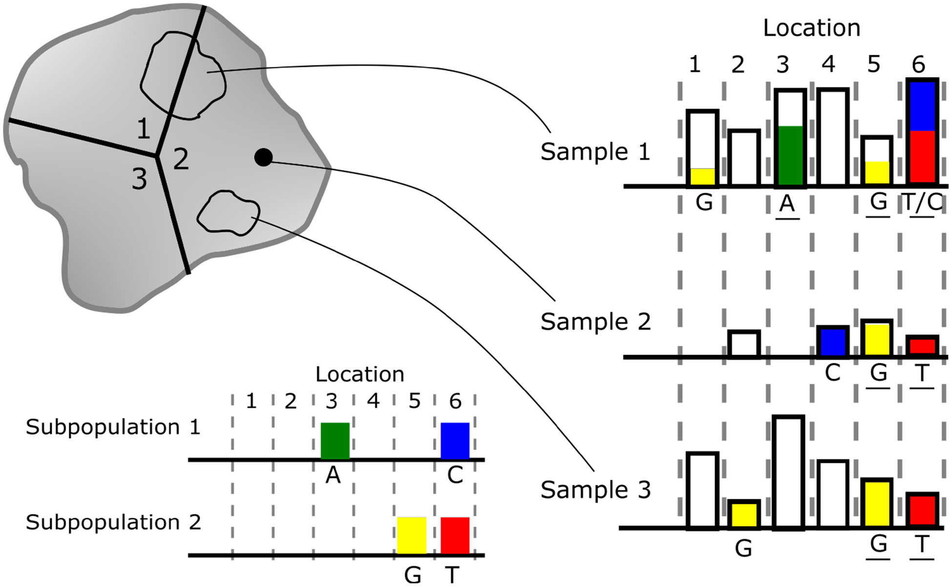
Prototypical example of tumor heterogeneity and clonal subpopulations.

1.1. Problem Setup.

The fundamental unit of sampling in NGS data is the read. A read is a short DNA sequence of 100–400 nucleobases (bases) that maps to a specific location in a reference genome; a typical DNA sequencing run produces millions of such reads. We denote the observed DNA base in read r ∈ {1, …, R_s} that maps to genomic location l ∈ {1, …, L} in sample s ∈ {1, …, S} as $x_{\mathit{\text{slr}}}\in \mathcal{B}=\{A,C,G,T\}$. Since there are only four DNA bases, we have a 1–1 mapping from $\mathcal{B}$ to {1, 2, 3, 4}. When a genomic location has only two bases that are observed in a population the location is called biallelic and the sample space can be reduced to x_slr ∈ {A, a}, where A is the major (most common) base and a is the minor (second most common) base. A read-count vector $n_{sl}={\left(n_{\mathit{\text{slb}}}\right)}_{b\in \mathcal{B}}$ can be constructed by summing over the reads and conditioning on a genomic location, $n_{\mathit{\text{slb}}}={\sum }_r\mathbb{1}\left[x_{\mathit{\text{slr}}}=b\right]$. The coverage at a given location is ${\sum }_{b\in \mathcal{B}}{n}_{\mathit{\text{slb}}}$. Goodwin, McPherson and McCombie (2016) present a comprehensive review of NGS, associated technologies, and summary statistics.

Single-cell sequencing data and bulk sequencing data differ in certain read-level statistics, but the fundamental observational unit for both is the read. DNA from single cells must be amplified by targeted amplification if a restricted region is of interest or whole genome amplification if the whole genome is of interest. The whole genome amplification process introduces false positives—apparent mutations that are not present in the original biological material and allelic dropout—heterogeneous alleles that appear homogeneous due to incomplete amplification of both alleles (Zafar et al., 2016). Both errors can be caused by founder effects due to early stage errors in polymerase chain reaction amplification. Additionally, single-cell sequencing data suffers from incomplete coverage of all loci and low sequencing depth (Zhang et al., 2019). In our problem setup each single-cell sample is treated as a single sample from the tumor.

Multiple NGS sequencing runs from an experiment are collected into a dataset, but the runs that comprise the dataset are rarely independent or identically distributed. In cancer sequencing datasets, there may be multiple individuals, each individual may have multiple solid tumors, and each solid tumor may have multiple biopsies. Data from model system experiments may have multiple genetic backgrounds and multiple environmental conditions. There may be multiple biological replicates and within each biological replicate there may be multiple technical replicates. A nested sampling structure produces samples that are correlated, and it is important to account for that correlation structure in the analysis of the data. In an experimental study, Paisley (2020) showed that a hierarchical Dirichlet process model performed better than a flat model when the number of samples at the lowest level of the sampling hierarchy was small. This data scenario is exactly the one we have with many NGS datasets.

1.2. Our contributions.

The goal of this work is to jointly infer the underlying genotypes of tumor subpopulations and the distribution of those subpopulations for each tumor sample by making use of both single-cell and bulk sequencing data from multiple tumor samples in multiple individuals. In Section 2 we propose a Bayesian nonparametric hierarchical Dirichlet process mixture model for combining information from bulk and single-cell next-generation DNA sequencing data from multiple samples and from multiple individuals. This hierarchical Dirichlet process mixture model has tunable hyperparameters that control the a priori concentration of the subpopulation distribution for each sample; this hyperparameter can be estimated in an empirical Bayes setting or set directly when the concentration is known— for example, when the sample is from a single-cell. The hierarchical structure models the nested sampling structure in real NGS datasets that arises from drawing multiple bulk and single-cell biopsies from multiple individuals. Inference with our model provides estimates of the subpopulation genotypes and the distribution over subpopulations in each sample. In Section 3 we represent the model as a Gamma-Poisson hierarchical model and in Section 4 we derive a fast Gibbs sampling algorithm based on this representation using the augment-and-marginalize method. This representation and inference algorithm are generalizable to other models that make use of a hierarchical Dirichlet process prior and can be employed to derive a fast Gibbs sampler with analytical sampling steps for other models.

This work aims to identify subpopulations that contain both somatic and germline mutations. In any tumor sample, some “normal” cells are likely to be present — these contain germline mutations, but not somatic mutations. Therefore, the normal subpopulation is a valid latent subpopulation in the context of our problem setup. Furthermore, germline mutations that are shared across multiple individuals in a study population will be evident in inferred latent subpopulation genotypes. We compare our model to related work on modeling heterogeneous NGS data using simulation experiments (Section 5) and we analyze real NGS data from a acute lymphoblastic leukemia (Section 6). Statistical inference provides estimates of the subpopulation genotypes and the distribution of subpopulations in individual samples with rigorous Bayesian uncertainty estimates. Since our inference algorithms produce samples from the full posterior distribution, our methods allow for rigorous quantification of the uncertainty in our estimates.

1.3. Related Work.

We briefly review related work in the area of Bayesian nonparametric modeling using the Dirichlet process and in the area of bioinformatic analysis of genetically heterogeneous samples.

1.3.1. Hierarchical Dirichlet Process Mixture Models.

In real data sets there is often structural information that can increase the utility of the data towards an inferential task. One of the most common pieces of structural information is the a priori similarity among related samples. As an example, suppose that we have a set of news articles and we are interested in drawing inferences about the topics in the articles. A näıve model might assume that all articles are independent samples; a more sophisticated model would incorporate information about the authorship—articles by the same author are a priori likely to be more similar to each other than to articles by different authors. In the Bayesian formalism, the hierarchical Dirichlet process enables one to incorporate such structural information in the inference process in a rigorous model-based way.

Dirichlet Process.

The Dirichlet process, G ~ DP(α₀,G₀), is formally a measure on measures where α₀ > 0 is the scaling parameter and G₀ is the base measure (Ferguson, 1973). A constructive definition is the stick-breaking representation (Sethuraman, 1994)

$$G=\sum _{k=1}^{\infty }{\pi }_k{\delta }_{{\varphi }_k},$$

where

$${\varphi }_k~G_0,{\pi }_k={\pi }_k^{\prime }\prod _{l=1}^{k-1}\left(1-{\pi }_l^{\prime }\right),{\pi }_k^{\prime }~\text{Beta}\left(1,{\alpha }_0\right).$$

The sequence $\pi ={\left({\pi }_k\right)}_{k=1}^{\infty }$ can be interpreted as a random probability measure on the positive integers and each integer is associated with a draw from the base measure. A second perspective of the Dirichlet process makes the clustering property more evident. The Chinese restaurant process (Aldous, 1985) describes a stochastic process where a draw θ_i associates with a parameter ϕ_k according to all of the previous pairs,

$${\theta }_i|{\theta }_1,\dots ,{\theta }_{i-1},{\alpha }_0,G_0~\sum _{k=1}^K\frac{m_k}{i-1+{\alpha }_0}{\delta }_{{\varphi }_k}+\frac{{\alpha }_0}{i-1+{\alpha }_0}{G}_0,$$

where m_k is the count of θ_i’s that are equal to ϕ_k. The conditional distribution is a mixture distribution where the weights are determined by the previous draws and α₀. If α₀ is large, the mixture distribution is weighted towards new draws from the base measure, G₀, and if α₀ is small, it was weighted towards previously sampled values of ϕ_k, where ϕ₁, …, ϕ_K are the distinct values taken on by θ₁, …, θ_i−1. For this reason, α₀ is called the concentration parameter of the Dirichlet process.

Dirichlet Process Mixture Model.

The Dirichlet process is a natural nonparametric prior for models that need a probability measure. In particular, it is useful for mixture models because they employ a probability measure as a latent or unobserved variable. In parametric models, a natural prior for this latent variable is a Dirichlet distribution. By substituting a Dirichlet process, the number of mixture components scales with the size of the data set and in the asymptotic limit of the sample size, n → ∞, the number of components goes to infinity, K → ∞. The Dirichlet process mixture model can be written as

$$\begin{array}{c}{\mathit{\theta }}_i|\mathit{\text{g}}~\mathit{\text{g}}\\ {\mathit{\text{x}}}_i|{\mathit{\theta }}_i~F\left({\mathit{\theta }}_i\right),\end{array}$$

where F(θ_i) is the sampling distribution of the observed data, x_i. The Dirichlet process mixture model can be construed as the infinite limit of a particular finite mixture model (Neal, 1992; Rasmussen, 2000; Green and Richardson, 2001; Ishwaran and Zarepour, 2002). The finite mixture model is

$$\begin{array}{cc}\mathit{\pi }|{\alpha }_0~\text{Dir}\left({\alpha }_0/K,\dots ,{\alpha }_0/K\right)\hfill & z_i|\mathit{\pi }~\mathit{\pi }\\ {\varphi }_k|G_0~G_0\hfill & x_i|z_i,{\left({\varphi }_k\right)}_{k=1}^K~F\left({\varphi }_{z_i}\right),\end{array}$$

where ϕ_k is the parameter for mixture component k drawn from prior distribution G₀, and z_i is an indicator of the mixture component. In the limit as K → ∞, this finite mixture model converges in distribution to the Dirichlet process mixture model (Ishwaran and Zarepour, 2002).

Hierarchical Dirichlet Process Mixture Model.

The hierarchical Dirichlet process is a hierarchical extension of the Dirichlet process mixture model where the prior over the mixing Dirichlet process is itself drawn from a Dirichlet process. Given a base measure H and concentration parameter γ, the hierarchical Dirichlet process mixture model is

$$\begin{array}{cc}{G}_0|\gamma ,H~\text{DP}(\gamma ,H)& G_j|{\alpha }_j,G_0~\text{DP}\left({\alpha }_j,G_0\right)\\ {\theta }_{ji}|G_j~G_j& x_{ji}|{\theta }_{ji}~F\left({\theta }_{ji}\right)\end{array}$$

This hierarchical stacking can be extended in the direction of the prior.

Combining information across related models.

Hierarchical Dirichlet process mixture models have the capacity to combine information across related samples. Müller, Quintana and Rosner (2004) describes two extremes for borrowing strength among related nonparametric submodels. At one extreme, the submodels are only linked through a fixed finite dimensional hyperparameter — in this case there is no borrowing of strength from data across submodels. At the other extreme, the models are linked through a common nonparametric base measure — in this case the data in the submodels is exchangeable. Between these extremes is a model where the submodel base measure is a mixture of a common measure and an independent measure (Müller, Quintana and Rosner, 2004). Another way to borrow strength from data across related submodels is through a shared prior as was done by Teh et al. (2006).

In our model, a common base measure is shared across all individual in the population. Conditional on that base measure, the biopsies within an individual are independent. The posterior measure for a particular individual is a combination of the prior measure over individuals and the data from the biopsies from that individual through the likelihood. Therefore, the hierarchical Dirichlet process mixture model proposed here lies between the two extremes outlined in Müller, Quintana and Rosner (2004), but in a way that reflects the experimental structure of this type of data.

1.3.2. Bioinformatic models for clonal subpopulation inference.

There are many methods for inferring the clonal genetic subpopulation structure from next-generation DNA sequencing data. A subset of these methods are based on a rigorous statistical model. We briefly review the most popular model-based bioinformatic methods for subpopulation structure inference. A more complete review of methods for subclonal inference is provided in Appendix A. PurityEst (Su et al., 2012) and PurBayes (Larson and Fridley, 2013) make use of paired tumor-normal samples. Roth et al. (2014) proposed a Dirichlet process mixture model for subpopulations called Pyclone. PhyloWGS uses a Bayesian nonparametric model to reconstruct genotypes of the subpopulations from sequencing data (Deshwar et al., 2015). Bayclone uses an Indian buffet process prior over the genotypes for the subpopulations (Sengupta et al., 2015). Sciclone uses a hierarchical Bayesian mixture model to infer subclonal populations (Miller et al., 2014). CloneHD integrates information from copy number data, B-allele frequency, and somatic nucleotide variants to infer clonal subpopulations (Fischer et al., 2014). Cloe takes the innovative approach of incorporating a prior over phylogenetic trees (Marass et al., 2016). Treeclone is a nonparametric Bayesian model for reconstructing the clonal subpopulation phylogeny and inferring tumor heterogeneity (Zhou et al., 2019).

Our work.

Our work handles multiple subpopulation components in the tumor unlike paired tumor-normal methods — paired data is not required. Like Pyclone, we use a Dirichlet process prior over the samples. Our model uses a simpler prior over the subpopulation genotypes compared to Bayclone, and uses a hierarchical Dirichlet process prior over the samples instead of an Indian buffet process. This modeling choice enables us to focus on posterior inference for the subpopulation genotypes and the distribution over genotypes.It has been shown that while the posterior distribution of the Dirichlet process is consistent, inference on the number of components is not (Miller and Harrison, 2013, 2014). For this reason, we focus on the posterior distribution of subpopulation genotypes and the posterior distribution of subpopulations for each sample.

2. Hierarchical Dirichlet Process Mixture Probability Model.

The full hierarchical Dirichlet process mixture model can be decomposed into the following components: the sampling model (Section 2.1), the hierarchical prior (Section 2.2), and the hyperparameters (Section 2.3). The full model and the complete posterior distribution is summarized in Section 2.4.

2.1. Sampling Model.

The model presented here assumes biallelic variants with the major allele denoted by A and the minor allele denoted by a, but the model is easily adapted for a situation where x_lsr records the observed DNA base {A, C, G, T}. The set of genotypes is denoted $\mathcal{G}\in \{AA,Aa,aa\}$ for a diploid genome and can equivalently be represented as $\mathcal{G}\in \{0,1,2\}$. We assume a conditional categorical sampling model for x_slr,

$$x_{\mathit{\text{slr}}}|z_{\mathit{\text{sr}}}~\text{\hspace{0.17em}Categorical\hspace{0.17em}}\left({\mathit{T}}_l^s\cdot {\mathit{h}}_{l{z}_{sr}}\right)$$ (1)

where

$$\begin{array}{cc}& \begin{array}{ccc}AA& Aa& aa\end{array}\\ {\mathit{T}}_l^s{=}_a^A& \left(\begin{array}{ccc}1-{ϵ}_{lA}^s& \frac{1}{2}& {ϵ}_{lq}^s\\ {ϵ}_{lA}^s& \frac{1}{2}& 1-{ϵ}_{la}^s\end{array}\right)\end{array},$$ (2)

is the genotype-base transition matrix. This matrix is typically the product of a sequencing error model and can be specified for a particular location l and for a particular sample s. The hyperparameters $\left\{{ϵ}_{lA}^s,{ϵ}_{la}^s\right\}$ can be estimated from historical data on the sequencing error rate at location l and set distinctly for bulk sequencing samples or single-cell samples due to the dependency on the sample s = (i, j).

The genotype for subpopulation k at location l is $h_{lk}\in \mathcal{G}$. The categorical variable h_lk can be equivalently represented by categorical indicator vector $h_{lk}\in {\{0,1\}}^{|\mathcal{G}|}$. The conditional distribution of the genotype of subpopulation k at location l is

$${\mathit{h}}_{lk}|{\mathit{a}}_l~\text{Multi}\left(1,{\mathit{a}}_l\right).$$ (3)

for all l = 1, …, L and k = 1, …, K. A simple independent prior for h_lk using Hardy-Weinberg equilibrium can be used, $a_{lk}=\left(\frac{1}{4},\frac{1}{2},\frac{1}{4}\right)$, or the prior should be adjusted based on population frequency information.

The integer-valued variable z_sr ∈ {1, 2, …, K} indicates the genetic subpopulation that produced read r in sample s. It has a categorical conditional distribution

$$z_{sr}|g_s~\text{\hspace{0.17em}Categorical}\left(g_s\right),$$ (4)

where g_s is the distribution over subpopulations for sample s.

2.2. Hierarchical Prior.

A key aspect of our model in the context of DNA sequencing datasets is a hierarchical Bayesian nonparametric prior on the distribution of subpopulations in sample s. Let sample s be generated by first drawing individual i = 1, …, N from a population and then drawing biopsy j = 1, …, N_i within individual i. Therefore, the sample is s ∈ {(i,j) | i = 1, …, N, j = 1, …, N_i}. The following hierarchical Dirichlet process prior is used for modeling g_s = g_ij,

$$g_{ij}~\text{DP}\left({\gamma }_{ij},g_i^{\prime }\right),(\text{distribution\hspace{0.17em}of\hspace{0.17em}subpopulations\hspace{0.17em}in\hspace{0.17em}biopsy\hspace{0.17em}}j)$$ (5)

$$g_i^{\prime }~\text{DP}\left({\beta }_i,g^{\prime \prime }\right),(\text{distribution\hspace{0.17em}of\hspace{0.17em}subpopulations\hspace{0.17em}in\hspace{0.17em}individual\hspace{0.17em}}i)$$ (6)

$$g^{\prime \prime }~\text{DP}\left({\alpha }_0,g^{\prime \prime \prime }\right).(\text{distribution\hspace{0.17em}of\hspace{0.17em}subpopulations\hspace{0.17em}in\hspace{0.17em}population)}$$ (7)

Here, g_ij is the distribution over subpopulations in biopsy j from individual i, $g_i^{\prime }$ is the distribution over subpopulations in individual i, and g″ is the distribution over subpopulations in the population from which the individuals are drawn. The top level prior measure g‴ together with the concentration parameter α₀ defines the prior over the population-level distribution of subpopulations. The products of inference in this model include the posterior distribution of these quantities.

2.3. Hyperparameters.

The hyperparameters α₀, β_i, and γ_ij are important for modeling single-cell and bulk sequencing experiments. If γ_ij is set to a small value, then g_ij is expected to be concentrated to one of the subpopulations. Therefore, if sample s = (i, j) is known to be from a single-cell, γ_ij can be set to a small value to represent an expected concentration to a single subpopulation. If the sequenced sample is a bulk of cells or an entire solid tumor, γ_ij can be set to a large value to represent an a-priori expectation of tumor heterogeneity. Hyperparameters α₀ and β_i represent prior information about subpopulation concentration at higher levels of the model. If β_i is set to a small value, the distribution of subpopulation for individual i is concentrated on a small number of subpopulations. Since g_ij is conditioned on $g_i^{\prime }$, the individual concentration parameter, β_i, influences the concentration of all of the biopsies within the individual. This hierarchical concentration in the model is congruent with the biological expectation that if a subpopulation is not present at the level of the individual, it would not emerge spontaneously in a sample from the individual. If α₀ is set to a small value, the subpopulation distribution is, a-priori, concentrated at only a few subpopulations. The inclusion/exclusion criteria for the dataset can therefore influence the concentration of the entire population. If the dataset contains only a small subset of the entire population, for example a subset of triple-negative breast cancer patients in a clinical trial, it may be reasonable to set α₀ to a small value. In the standard Bayesian paradigm, if the concentration parameter is not known a-priori, the associated parameters can be endowed with a Gamma distribution as in Escobar and West (1995).

2.4. Complete Hierarchical Dirichlet Process Model.

By combining the sampling model and the hierarchical prior the complete hierarchical Dirichlet process model is

$$\begin{array}{cc}{h}_{lk}~\text{Multi}\left(1,a_l\right),& \hfill \text{for\hspace{0.17em}each\hspace{0.17em}}(l,k),\\ g^{\prime \prime }|{\alpha }_0,g^{\prime \prime \prime }~\text{DP}\left({\alpha }_0,g^{\prime \prime \prime }\right),& \hfill \\ g_i^{\prime }|\beta i,g^{\prime \prime }~\text{DP}\left({\beta }_i,g^{\prime \prime }\right),& \hfill \text{for\hspace{0.17em}each\hspace{0.17em}}i,\\ g_{ij}|{\gamma }_{ij},g_i^{\prime }~\text{DP}\left({\gamma }_{ij},g_i^{\prime }\right),& \hfill \text{for\hspace{0.17em}each\hspace{0.17em}}(i,j),\\ z_{ijr}|g_{ij}~\text{\hspace{0.17em}Categorical\hspace{0.17em}}\left(g_{ij}\right),& \hfill \text{for\hspace{0.17em}each\hspace{0.17em}}(i,j,r),\\ x_{\mathit{\text{lijr}}}|z_{ijr},h_l~\text{\hspace{0.17em}Categorical\hspace{0.17em}}\left(T_l^{(i,j)}\cdot h_{l{z}_{\mathit{\text{ijr}}}}\right),& \hfill \text{for\hspace{0.17em}each\hspace{0.17em}}(l,i,j,r).\end{array}$$ (hDP)

A graphical model representation of Model hDP is shown in Figure 2. Model hDP is conceptually compared with other common hierarchical models for factorizing count data in Appendix D.

Fig 2:

Graphical model representation of Model hDP.

The object of inference is the posterior distribution function for Model hDP:

$$p\left(h,g^{\prime \prime },g^{\prime },g,z|x;a,g^{\prime \prime \prime },{\alpha }_0,\beta ,\gamma ,T\right)\propto p\left(g^{\prime \prime }|g^{\prime \prime \prime },{\alpha }_0\right)\prod _{i=1}^{N}p\left(g_i^{\prime }|g^{\prime \prime },{\beta }_i\right)$$

$$\prod _{j=1}^{N_i}p\left(g_{ij}|g_i^{\prime },{\gamma }_{ij}\right)\prod _{r=1}^{R_{ij}}p\left(z_{\mathit{\text{ijr}}}|g_{ij}\right)\prod _{l=1}^{L}p\left(x_{\mathit{\text{lijr}}}|z_{\mathit{\text{ijr}}},T_l^{(i,j)},h_l\right)p\left(h_l|a_l\right).$$

Next, we derive a Markov chain Monte Carlo (MCMC) inference algorithm to estimate this posterior distribution.

2.5. Inference Algorithm for Hierarchical Dirichlet Process Model.

It is well-known that a Dirichlet distribution with parameter $\frac{\alpha }{K}$ converges to a Dirichlet process as K → ∞ (Teh et al., 2006; Ishwaran and Zarepour, 2000). We employ this fact to derive an MCMC algorithm to draw samples from the posterior distribution. The details of the derivation of the truncated Dirichlet process inference algorithm are in Appendix B. The algorithm itself is shown in Algorithm 1.

Algorithm 1:

MCMC sampler for Model hDP

3. Hierarchical Gamma-Poisson Probability Model.

The inference algorithm for Model hDP employs Metropolis-Hastings steps that can be computationally expensive for large datasets. To address this issue, we reformulate the model as a hierarchical Gamma-Poisson model. This reformulation allows us to use the augment-and-marginalize method developed by Zhou et al. (2012) to derive a fast inference algorithm that uses only analytical sampling steps for updates.

3.1. Sampling Model.

In the hierarchical Dirichlet process model, the observed data is the base for each read; in this Gamma-Poisson reformulation, the observed data is count of reads associated with each base. Let Y_ijlb ∈ {0, 1, 2, …} be the read count of base $b\in \mathcal{B}$ at location l ∈ {1, …, L} in biopsy j ∈ {1, …, N_i} of individual i ∈ {1, …, N} (recall we have defined a sample as the pair s = (i, j)). We assume the read count has a conditional Poisson distribution,

$$y_{\mathit{\text{ijlb}}}|{\theta }_{\mathit{\text{ijk}}},{\varphi }_{\mathit{\text{lbk}}}~\text{Pois}\left(\sum _{k=1}^K{\theta }_{\mathit{\text{ijk}}}{\varphi }_{\mathit{\text{lbk}}}\right).$$ (8)

Note that while the conditional distribution is Poisson, the marginal distribution is negative binomial as shown in Equation (15). The rate parameter of the Poisson is a sum over K subpopulations where the summand is the product of two factors. The first factor θ_ijk is the rate or propensity of subpopulation k in sample s = (i, j). The second factor is ϕ_lbk ≜ (T_l ·h_lk)_b ∈ (0, 1) and can be interpreted as the probability of base b in subpopulation k at location l. This representation requires the same genotype-nucleobase transition matrix across all samples.

3.2. Hierarchical Prior.

We assume the following hierarchical gamma prior for propensity θ_ijk:

$$\begin{array}{cc}{\theta }_{ijk}~\mathrm{\Gamma }\left({\theta }_{ik}^{\prime },1\right),& \hfill (\text{propensity\hspace{0.17em}of\hspace{0.17em}subpopulation\hspace{0.17em}}k\text{\hspace{0.17em}in\hspace{0.17em}biopsy\hspace{0.17em}}j\text{\hspace{0.17em})}\\ {\theta }_{ik}^{\prime }~\mathrm{\Gamma }\left({\theta }_k^{\prime \prime },1\right),& \hfill (\text{propensity\hspace{0.17em}of\hspace{0.17em}subpopulation\hspace{0.17em}}k\text{\hspace{0.17em}in\hspace{0.17em}individual\hspace{0.17em}}i)\\ {\theta }_k^{\prime \prime }~\mathrm{\Gamma }\left({\rho }_0/K,\tau \right),& \hfill (\text{propensity\hspace{0.17em}of\hspace{0.17em}subpopulation\hspace{0.17em}}k\text{\hspace{0.17em}in\hspace{0.17em}population)}\\ {\rho }_0,\tau ~\mathrm{\Gamma }\left({ϵ}_0,{ϵ}_0\right).& \hfill (\text{latent\hspace{0.17em}parameters)}\end{array}$$ (9)

The form of the gamma distribution is Γ(a, b) where a is the shape parameter and b is the rate parameter. While the gamma distribution is the conjugate prior to its own rate parameter, this hierarchical prior is in a non-conjugate configurations since it chains through the shape parameter. Nevertheless, this construction yields closed-form complete conditional distributions via an auxiliary variable augment-and-marginalize update that is derived in Section 4.

3.3. Hyperparameters.

The hyperparameter ϵ₀ can be set to a small value for a diffuse prior over the parameters ρ₀ and τ. If it is known that the entire data set is relatively concentrated on only one subpopulation ϵ₀ can be set to a smaller value such as one. Or, if there is a priori information about the expected number of subpopulations, the shape and rate parameters can be adjusted accordingly. The distributions are not restricted to depend on a single hyperparameter.

3.4. Complete Gamma-Poisson Model.

The complete Gamma-Poisson model is

$$\begin{array}{cc}{h}_{lk}~\text{Multi}\left(1,a_l\right),& \hfill \text{for\hspace{0.17em}each\hspace{0.17em}}l,\\ {\rho }_0,\tau ~\mathrm{\Gamma }\left({ϵ}_0,{ϵ}_0\right),& \hfill \\ {\theta }_k^{\prime \prime }~\mathrm{\Gamma }\left({\rho }_0/K,\tau \right),& \hfill \text{for\hspace{0.17em}each\hspace{0.17em}}k,\\ {\theta }_{ik}^{\prime }~\mathrm{\Gamma }\left({\theta }_k^{\prime \prime },1\right),& \hfill \text{for\hspace{0.17em}each\hspace{0.17em}}(i,k),\\ {\theta }_{ijk}~\mathrm{\Gamma }\left({\theta }_{ik}^{\prime },1\right),& \hfill \text{for\hspace{0.17em}each\hspace{0.17em}}(i,j,k),\\ y_{\mathit{\text{ijlb}}}~\text{Pois}\left(\sum _{k=1}^K{\theta }_{\mathit{\text{ijk}}}{\varphi }_{\mathit{\text{lbk}}}\right),& \hfill \text{for\hspace{0.17em}each\hspace{0.17em}}(l,i,j,b).\end{array}$$ (hGP)

This model trades model flexibility for computational efficiency. The transition matrix T_l is fixed for all samples and there is no tunable prior subpopulation concentration of each sample, but the computational efficiency of the resulting inference algorithm is significantly better than the hierarchical Dirichlet process mixture model and this model can be fit to much larger data sets. A complete graphical model representation of Model hGP is shown in Figure 3.

Fig 3:

Graphical model representation of Model hGP.

The complete posterior distribution of the data under the Gamma-Poisson model is

$$\begin{gathered} p\left(\theta ,{\theta }^{\prime },{\theta }^{\prime \prime },{\rho }_0,\tau |y;a,T,{ϵ}_0\right)\propto p\left({\rho }_0,\tau |{ϵ}_0\right)\prod _{k=1}^{\text{K}}p\left({\theta }_k^{\prime \prime }|{\rho }_0,\tau \right)\prod _{i=1}^{N}p\left({\theta }_{ik}^{\prime }|{\theta }_k^{\prime \prime }\right). \\ \prod _{j=1}^{N_j}p\left({\theta }_{\mathit{\text{ijk}}}|{\theta }_{\mathit{\text{ik}}}^{\prime }\right)\prod _{l=1}^{L}p\left(h_{lk}|a_l\right)\prod _{b\in \mathcal{B}}p\left({\varphi }_{\mathit{\text{lbk}}}|T_l,h_{lk}\right)p\left(y_{\mathit{\text{ijlb}}}|{\theta }_{\mathit{\text{ijk}}},{\varphi }_{\mathit{\text{lbk}}}\right). \end{gathered}$$ (10)

3.5. Interpretation as a Hierarchical Dirichlet Process Mixture Model.

The hierarchical prior in Equation (9) can be interpreted in terms of a hierarchical Dirichlet process, similar to that given in Section 2.2. To see this, we appeal to (1) the relationship between the Gamma and Dirichlet distributions, and (2) the limiting form of the finite-dimensional Dirichlet distribution as the number of subpopulations goes to infinity.

A sample from a Dirichlet distribution can be obtained by normalizing a vector of independent gamma random variables with equal rate parameters but possibly different shape parameters. Suppose θ_k ~ Γ(a_k, 1) for k = 1, …, K are K independent Gamma random variables with shape parameters a_k. We adopt dot (·) notation $\theta .={\sum }_{k=1}^K{\theta }_k$ to denote sums. We denote proportion vector $\tilde{\theta }=\left({\tilde{\theta }}_1,\dots ,{\tilde{\theta }}_K\right)$ where ${\tilde{\theta }}_k=\frac{{\theta }_k}{\theta .}$. Lukacs (1955) showed that θ. and $\tilde{\theta }$ are then marginally (i.e., not conditional on θ₁, …, θ_K) independent; moreover, they are distributed as θ. ~ Γ(a., 1), where $a.={\sum }_{k=1}^K{a}_k$, and $\tilde{\theta }~\text{Dir}(a.,\tilde{a})$, where $\tilde{a}=\left(\frac{a_1}{a.},\dots ,\frac{a_K}{a.}\right)$.

Because of the relationship between the gamma and Dirichlet random variables, the propensity θ_ijk can be represented as

$${\theta }_{\mathit{\text{ijk}}}={\theta }_{ij}\cdot {\tilde{\theta }}_{\mathit{\text{ijk}}},$$

Where

$${\theta }_{ij\cdot }~\mathrm{\Gamma }\left({\theta }_{i\cdot }^{\prime },1\right)\text{\hspace{1em}and\hspace{1em}}{\tilde{\theta }}_{ij}~\text{Dir}\left({\theta }_{i\cdot }^{\prime },{\tilde{\theta }}_i^{\prime }\right).$$

Likewise, we can represent ${\theta }_{ik}^{\prime }$ as

$${\theta }_{ik}^{\prime }={\theta }_{i\cdot }^{\prime }{\tilde{\theta }}_{ik}^{\prime },\text{\hspace{1em}where\hspace{1em}}{\theta }_{i\cdot }^{\prime }~\mathrm{\Gamma }\left({\theta }_{\cdot }^{\prime \prime },1\right)\text{\hspace{1em}and\hspace{1em}}{\tilde{\theta }}_i^{\prime }~\text{Dir}\left({\theta }_{\cdot }^{\prime \prime },{\tilde{\theta }}^{\prime \prime }\right);$$

and we can represent ${\theta }_k^{\prime \prime }$ as

$${\theta }_k^{\prime \prime }={\theta }^{\prime \prime }{\tilde{\theta }}_k^{\prime \prime },\text{\hspace{1em}where\hspace{1em}}{\theta }_{\cdot }^{\prime \prime }~\mathrm{\Gamma }\left({\rho }_0,\tau \right)\text{\hspace{1em}and\hspace{1em}}{\tilde{\theta }}^{\prime \prime }~\text{Dir}\left({\rho }_0,\left(\frac{1}{K},\dots ,\frac{1}{K}\right)\right).$$

At each level in the hierarchy, we independently sample the sum from a gamma distribution and the proportions vector from a Dirichlet distribution The product of these yields a sample of the conditionally independent propensity value at that level.

This representation induces a hierarchical of Dirichlet prior over the proportions vectors at each level. Taking K → ∞, that hierarchical Dirichlet prior then describes the prior over the weights of the following hierarchical Dirichlet process (HDP):

$$g_{ij}=\sum _{k=1}^{\infty }{\mathbb{1}}_{{\varphi }_k}{\tilde{\theta }}_{\mathit{\text{ijk}}}~\text{DP}\left({\theta }_{i\cdot }^{\prime },g_i^{\prime }\right),$$

$$g_i^{\prime }=\sum _{k=1}^{\infty }{\mathbb{1}}_{{\varphi }_k}{\tilde{\theta }}_{ik}^{\prime }~\text{DP}\left({\theta }_{\cdot }^{\prime \prime },{\mathit{g}}^{\prime \prime }\right),$$

$$g^{\prime \prime }=\sum _{k=1}^{\infty }{\mathbb{1}}_{{\varphi }_k}{\tilde{\theta }}_k^{\prime \prime }~\text{DP}\left({\rho }_0,g^{\prime \prime \prime }\right),$$

where g‴ is the base measure. This HDP prior is the same as the HDP prior in Section 2.2 except that the concentration parameters (e.g., ${\theta }_{\cdot }^{\prime \prime }$) are gamma random variables, as opposed to fixed hyperparameters, and are shared across all random variables at a given level.

4. Augment-and-Marginalize Gibbs Sampling for Gamma–Poisson Model.

In this section the complete conditional distributions are derived for all latent variables in the Gamma-Poisson model—iteratively sampling from these constitutes a Markov chain whose stationary distribution is the exact posterior. The complete conditionals for all latent variables are available in closed form when further conditioned on a set of auxiliary variables. These auxiliary variables have closed form conditional distributions while leaving the stationary distribution of the Markov chain invariant; thus they facilitate efficient Gibbs sampling inference.

4.1. Latent subcounts.

As with most Gamma-Poisson models, the first set of auxiliary variables that facilitate inference are the latent sub-counts y_ijlb1, …, y_ijlbK which sum to the observed count $y_{\mathit{\text{ijlb}}}={\sum }_{k=1}^K{y}_{\mathit{\text{ijlbk}}}$. The k^th subcount y_ijlbk represents the number of reads in sample s = (i, j) at locus l of base b that are allocated to latent subpopulation k. When conditioned on their sum, the vector of sub-counts is Multinomial-distributed:

$${\left(y_{\mathit{\text{ijlbk}}}\right)}_{k=1}^K|y_{\mathit{\text{ijlb}}},{\theta }_{\mathit{\text{ijk}}},{\varphi }_{\mathit{\text{blk}}}~\text{Multi\hspace{0.17em}}\left(y_{\mathit{\text{ijlb}}},{\left(\frac{{\theta }_{\mathit{\text{ijk}}}{\varphi }_{\mathit{\text{blk}}}}{{\sum }_{k^{\prime }=1}^K{\theta }_{{\mathit{\text{ijk}}}^{\prime }}{\varphi }_{{\mathit{\text{blk}}}^{\prime }}}\right)}_{k=1}^K\right).$$ (11)

The complete conditionals of the other latent variables depend on different sums of these latent subcounts. Consider the total count of reads in sample s = (i, j) allocated to subpopulation k:

$$y_{ij\cdot \cdot k}\triangleq \sum _{l=1}^L\sum _{b\in \mathcal{B}}{y}_{\mathit{\text{ijlbk}}}.$$ (12)

Due to the additive property of the Poisson distribution, this count is Poisson-distributed in the generative model:

$$y_{ij\cdot \cdot k}|\theta ,\varphi ~\text{Pois}\left(\sum _{l=1}^L\sum _{b\in \mathcal{B}}{\theta }_{\mathit{\text{ijk}}}{\varphi }_{\mathit{\text{blk}}}\right).$$ (13)

Since ${\sum }_{b\in \mathcal{B}}{\varphi }_{\mathit{\text{blk}}}=1$ this simplifies to

$$y_{ij\cdot \cdot k}|\theta ~\text{Pois}\left(L{\theta }_{\mathit{\text{ijk}}}\right).$$ (14)

4.2. Augment-and-marginalize.

Although this model posits a non-conjugate hierarchical Gamma prior, we can apply the “augment-and-conquer” procedure of Zhou and Carin (2012) to recursively marginalize out Gamma random variables and augment the model with auxiliary count variables to obtain closed-form conditionals for all latent variables. At a high level, the idea of augmentation is to represent a single complex distribution as a compound distribution such that when the compound distribution is appropriately marginalized the result is the original complex distribution. A simple example is the Student’s T distribution, which can be represented as a Gaussian distribution with an inverse Gamma prior on the variance parameter: when the variance is marginalized out, the result is a Student’s T distribution.

Marginalize θ_ijk.

The Poisson variable in Equation (14) represents the count of all reads whose distribution directly depends on θ_ijk. Marginalizing out θ_ijk gives a negative binomial distribution over y_ij··k:

$$y_{ij\cdot \cdot k}|{\theta }_{ik}^{\prime }~\text{NegBinom}\left({\theta }_{ik}^{\prime },\frac{L}{1+L}\right).$$ (15)

We note that previous work has shown that DNA sequencing count data is well-represented by a negative binomial distribution (Rabadan et al., 2018).

Augment with w_ijk.

If we now augment the model with the following Chinese Restaurant Table (CRT) random variable,

$$w_{ijk}|y_{ij\cdot \cdot k},{\theta }_{ik}^{\prime }~\text{CRT}\left(y_{ij\cdot \cdot k},{\theta }_{ik}^{\prime }\right),$$ (16)

then the bivariate distribution $p\left(y_{ij\cdot \cdot k},w_{\mathit{\text{ijk}}}|{\theta }_{ik}^{\prime }\right)$ can be equivalently factorized as

$$w_{\mathit{\text{ijk}}}|{\theta }_{ik}^{\prime }~\text{Pois}\left({\theta }_{ik}^{\prime }\text{\hspace{0.17em}log}(1+L)\right),$$ (17)

$$y_{ij\cdot \cdot k}|w_{ijk}~\text{SumLog}\left(w_{ijk},\frac{L}{1+L}\right),$$ (18)

where SumLog(w, p) is the distribution of the sum of w i.i.d. Logarithmic random variables with probability parameter p. The Chinese restaurant table (CRT) distribution is the distribution of the number of nonempty tables in a Chinese restaurant process (Zhou and Carin, 2015). Suppose we have a Chinese restaurant process with concentration parameter ρ₀ and m customers. Then, the number of occupied tables is $l={\sum }_{i=1}^m{b}_i$ where $b_i~\text{Bernoulli\hspace{0.17em}}\left(\frac{{\rho }_0}{i-1+{\rho }_0}\right)$ and the distribution of l is l ~ CRT(m, ρ₀).

Inference in Augmented Model.

A graphical model representation of the augment-and-marginalize procedure is shown in Figure 4. Figure 4a shows the original model structure with non-conjugate prior and Figure 4d shows the equivalent model structure where conjugacy holds. During inference, we sample the auxiliary variable w_ijk using Equation (16). We may then proceed under the assumption that w_ijk was in fact drawn from Equation (17) and that all dependence of $y_{ij}^{(k)}$ on ${\theta }_{ik}^{\prime }$ flows through w_ijk. By marginalizing out θ_ijk and augmenting with w_ijk we have replaced a non-conjugate link from ${\theta }_{ik}^{\prime }$ to θ_ijk with a conjugate link from ${\theta }_{ik}^{\prime }$ to w_ijk. In the next steps, we recurse up the hierarchy.

Fig 4:

Augment-and-marginalize steps. (a) The original model structure. (b) The modelis transformed by marginalizing over θ_ijk. (c) The model is augmented with the Chinese restaurant table (CRT) random variable w_ijk. (d) Finally, the joint distribution $p\left(y_{ij\cdot \cdot k},w_{ijk}|{\theta }_{ik}^{\prime }\right)$ can be factorized using into the product of a Poisson and SumLog distribution.

Marginalize ${\theta }_{ik}^{\prime }$.

Having marginalized θ_ijk, we now move up the model hierarchy to ${\theta }_{ik}^{\prime }$. Define the $w_{ik}\triangleq {\sum }_{j=1}^{N_i}{w}_{\mathit{\text{ijk}}}$ which is Poisson distributed,

$$w_{ik}|{\theta }_{ik}^{\prime }~\text{Pois}\left({\theta }_{ik}^{\prime }{N}_i\text{\hspace{0.17em}log}(1+L)\right).$$

This count isolates the dependence of downstream variables on ${\theta }_{ik}^{\prime }$, allowing us to marginalize ${\theta }_{ik}^{\prime }$ out—doing so induces the following negative binomial distribution over w_ik:

$$w_{ik}|{\theta }_k^{\prime \prime }~\text{NegBinom}\left({\theta }_k^{\prime \prime },\frac{N_i\text{\hspace{0.17em}log}(1+L)}{1+N_i\text{\hspace{0.17em}log}(1+L)}\right)$$

Augment with $w_{ik}^{\prime }$.

We augment the model with a CRT variable,

$$w_{ik}^{\prime }|w_{ik},{\theta }_k^{\prime \prime }~\text{CRT}\left(w_{ik},{\theta }_k^{\prime \prime }\right),$$

and then re-represent the bivariate distribution of w_ik and $w_{ik}^{\prime }$ as:

$$w_{ik}^{\prime }|{\theta }_k^{\prime \prime }~\text{Pois}\left({\theta }_k^{\prime \prime }\text{\hspace{0.17em}log}\left(1+N_i\text{\hspace{0.17em}log}(1+L)\right)\right)$$ (19)

$$w_{ik}|w_{ik}^{\prime }~\text{SumLog}\left(w_{ik}^{\prime },\frac{N_i\text{\hspace{0.17em}log}(1+L)}{1+N_i\text{\hspace{0.17em}log}(1+L)}\right).$$ (20)

Marginalize ${\theta }_k^{\prime \prime }$.

We now recurse up the hierarchy again. Defining the sum $w_k^{\prime }\triangleq {\sum }_{i=1}^N{w}_{ik}^{\prime }$, which is Poisson distributed:

$$w_k^{\prime }|{\theta }_k^{\prime \prime }~\text{Pois}\left({\theta }_k^{\prime \prime }N\text{\hspace{0.17em}log}\left(1+N_i\text{\hspace{0.17em}log}(1+L)\right)\right).$$

Marginalizing out ${\theta }_k^{\prime \prime }$ induces a negative binomial distribution:

$$w_k^{\prime }|{\rho }_0,\tau ~\text{NegBinom}\left({\rho }_0/K,\frac{N\text{\hspace{0.17em}log}\left(1+N_i\text{\hspace{0.17em}log}(1+L)\right)}{\tau +N\text{\hspace{0.17em}log}\left(1+N_i\text{\hspace{0.17em}log}(1+L)\right)}\right)$$

Augment with $w_k^{\prime \prime }$.

We augment the model with another CRT variable,

$$w_k^{\prime \prime }|g_k^{\prime },{\rho }_0~\text{CRT}\left(w_k^{\prime },{\rho }_0/K\right),$$

and then re-represent the bivariate distribution of $w_{ik}^{\prime }$ and $w_{ik}^{\prime \prime }$ as:

$$w_k^{\prime \prime }|{\rho }_0,\tau ~\text{Pois}(\left({\rho }_0/K\right)(\text{log}\left(1+N\text{\hspace{0.17em}log}\left(1+N_i\text{\hspace{0.17em}log}(1+L)\right)/\tau \right)$$ (21)

$$w_k^{\prime }|w_k^{\prime \prime }~\text{SumLog}\left(w_k^{\prime \prime },\frac{N\text{\hspace{0.17em}log}\left(1+N_i\text{\hspace{0.17em}log}(1+L)\right)}{\tau +N\text{\hspace{0.17em}log}\left(1+N_i\text{\hspace{0.17em}log}(1+L)\right)}\right).$$ (22)

Doing so admits a conjugate link between ρ₀ and $w_k^{\prime \prime }$.

4.3. Algorithm.

The augment-and-marginalize derivation in the previous section involves introducing auxiliary variables which replace the non-conjugate links in the model with conjugate ones. This leads to an “upwards-downwards” Gibbs sampler in which we first sample auxiliary CRT counts up the hierarchy, then sample Gamma variables from conjugate conditionals down the hierarchy. A complete algorithm for the the Gibbs sampler for the Poisson-Gamma model is in Appendix C.

5. Simulation Experiments.

In the previous sections we presented a novel hierarchical Dirichlet process mixture model for combining single-cell and bulk sequencing data and using the correlation between related samples induced by the sampling strategy or experimental design. The hierarchical Dirichlet process mixture model (Model hDP) allows for direct control over the a priori concentration of the sample, but the inference algorithm requires expensive Metropolis-Hastings steps. The hierarchical Gamma-Poisson model (Model hGP) can be interpreted as representation of the hierarchical Dirichlet process mixture model closely related to Model hDP with a much faster inference algorithm only requiring Gibbs sampling from analytical distributions. In this section, measure the accuracy, computational efficiency, and stability of these models compared to state-of-the-art machine learning and bioinformatics methods.

Data Generation.

Simulation data was generated from a parametric hierarchical Dirichlet mixture model with K = 3 true subpopulations and L = 5 genomic locations. The number of individuals is N = 6 and each individual has 1 bulk sample and 3 single-cell samples for a total of N_i = 4 biopsies for each individual. The number of reads per sample (across 5 genomic locations) is R_ij = 100; each genomic location has an average of 20 reads. Simulation data was generated according to the following model:

$$g^{\prime \prime }~\text{Dir}(\alpha ),g_i^{\prime }~\text{Dir}\left({\beta }_i\cdot g^{\prime \prime }\right),g_{ij}~\text{Dir}\left({\gamma }_{ij}\cdot g_i^{\prime }\right),$$

$$z_{\mathit{\text{ijr}}}~\text{Categorical\hspace{0.17em}}\left(g_{ij}\right),x_{\mathit{\text{ijlr}}}~\text{Categorical\hspace{0.17em}}\left(T_l^{(ij)}\cdot h_{l{z}_{\mathit{\text{ijr}}}}\right),$$

where α = (1, 1, 1), β_i = 1, and γ_ij = 10 for the bulk samples and γ_ij = 0.1 for the single-cell samples. The genotype-nucleotide transition matrix is

$$\begin{array}{cc}& \begin{array}{ccc}AA& Aa& aa\end{array}\\ {\mathit{T}}_l^{(ij)}{=}_a^A& \left(\begin{array}{ccc}1-{ϵ}_{lA}^{(ij)}& \frac{1}{2}& {ϵ}_{la}^{(ij)}\\ {ϵ}_{lA}^{(ij)}& \frac{1}{2}& 1-{ϵ}_{la}^{(ij)}\end{array}\right)\end{array},$$

where ${ϵ}_{la}^{(\text{bulk})}={ϵ}_{lA}^{(\text{bulk})}=0.01$ and ${ϵ}_{la}^{(\text{sc})}={ϵ}_{lA}^{(\text{sc})}=0.15$ for bulk and single-cell samples respectively—(bulk) ≜ {s = (i, j) | j is a bulk sample} and (sc) ≜ {s = (i, j) | j is a single-cell sample}. As a benchmark, the subpopulationgenotype matrix is set to

$$h^{\top }=\left[\begin{array}{lllll}2\hfill & 2\hfill & 0\hfill & 0\hfill & 0\hfill \\ 0\hfill & 0\hfill & 2\hfill & 0\hfill & 0\hfill \\ 0\hfill & 0\hfill & 0\hfill & 2\hfill & 2\hfill \end{array}\right]$$

and in other simulation experiments h is randomly sampled from a prior distribution.

Posterior Inference.

The marginal posterior distributions g″|x, g′|x, g′|x and h were estimated using MCMC samples generated from Algorithm 1. We sampled 490 posterior samples after a burn-in/warm-up of 1,000 samples and thinning by a factor of 100. The number of subpopulations in the truncated Dirichlet process mixture inference algorithm (Algorithm 1) is set to K = 30 which is a factor of 10 greater than the true number of subpopulations. Figure 1 shows the true values and posterior distribution estimates from the simulation model, where the top three components of the model finds are exactly the same as the three components of h and the fourth component of the model finds has nearly zero probability. At population level, the KL divergence between the true distribution and inferred posterior distribution is $\text{KL}\left(g^{\prime \prime }\Vert {\widehat{g}}^{\prime \prime }\right)=0.570$. At individual level, the average KL divergence is $\frac{1}{N}{\sum }_{i=1}^N\text{KL}\left(g_i^{\prime }\Vert {\widehat{g}}_i^{\prime }\right)=0.692$ and the standard deviation is 0.289. At the biopsy level, the average KL divergence is $\frac{1}{N}{\sum }_{i=1}^N\frac{1}{N_i}{\sum }_{i=1}^N\text{KL}\left(g_{ij}\Vert {\widehat{g}}_{ij}\right)=0.521$ and the standard deviation is 0.371. A detailed visualization and discussion of the posterior distribution are in Appendix D.1. These results indicate that the model is able to identify the true subpopulation genotypes and the posterior distributions are appropriately uncertain relative to the amount of data and the proximity to the data in the model.

Comparison to LDA and NNMF.

To assess the importance of the hierarchical structure in Model hDP, we compared the performance to latent Dirichlet allocation (LDA) and non-negative matrix factorization (NNMF). However, both LDA and NNMF failed to find the true components for our benchmark simulation data. Thus we generated other data sets using the same parametric model but only having bulk data and compared the performance with our model. The KL divergence, $\text{KL}\left(g_{ij}\Vert {\widehat{g}}_{ij}\right)$, mean and 95% confidence interval across inference repeats is shown in Figure 2 in Appendix D.2 (Table 1 in Appendix D.2 shows the numerical values). These experiments shows that Model hDP outperforms LDA and NNMF for bulk-only and mixed data scenarios.

Comparison to PhyloWGS and TreeClone.

We compared the performance of Model hDP to two other models for inferring clonal subpopulations in mixed samples: PhyloWGS and TreeClone. Due to sample size limitations in PhyloWGS, we reduced the sample size to N ∈ {1, 2}), N_i ∈ {1, 2, 3} and only generated bulk data and kept other settings same (R_ij=100, L=5) to generate 6 simulation datasets to compare PhyloWGS, TreeClone and Model hDP. PhyloWGS successfully identifies true subpopulations at sample level but inferred an incorrect hierarchical structure relating the samples. A complete presentation of the results of this experiment are in Appendix D.3. Figure 3 therein shows phyloWGS’s posterior distributions at sample level are less accurate than Model hDP in terms of KL divergence. TreeClone successfully identifies number of subpopulations but the posterior distributions at sample level are less accurate than our model.

Sensitivity Analysis.

To assess the sensitivity of the model, we performed simulation experiments varying h, K, L, and the single-cell sequencing error rate ${ϵ}_{lA}^{(ij)}$ and ${ϵ}_{lA}^{(ij)}$. To assess the sensitivity to different values of h, five simulation data sets were randomly generated with h_lk ~ Multi(1, a) where a = (0.45, 0.1, 0.45). In all cases, the model was able to identify the true subpopulation genotypes when the subpopulation was represented by samples in the data as shown in Appendix E.1. To assess the sensitivity to varying K, K was increased from 3 to 10 with L = 10 and R_ij = 1000 with randomly sampled h. Appendix E.2 shows the results of the simulation experiment of vary K: our model successfully inferred true components with relatively small KL divergence. To assess the sensitivity to varying L, we ran simulation experiments with L = {3, 10, 20, 50, 100}. Appendix E.3 shows our model identified the subpopulations and posterior distribution of the subpopulations across this range of L. Finally, we assessed the sensitivity of the model to varying single-cell sequencing error rate ${ϵ}_{lA}^{(ij)}$ for the single-cell samples because while the error rate for bulk experiments is well-established, the error rate for single-cell experiments is more uncertain. We set ${ϵ}_{lA}^{(ij)}=\{0.1,0.15,0.2,0.25,0.3\}$ and sampled h randomly. The results (Appendix E.4) show our model was not sensitive to the specified single-cell sequencing error rate, but performance does degrade as the error rate increases.

Accuracy and Computational Efficiency of Model hGP.

Since Model hGP is designed for a large number of single-cell samples, we simulated N_i = 99 single-cell samples from the benchmark model with a sequencing error rate of ${ϵ}_{lA}^{(ij)}={ϵ}_{lA}^{(ij)}=0.15$. The model took less than 10 minutes to run and identified all three subpopulation genotypes exactly, $\Vert \mathit{h}-\widehat{\mathit{h}}{\Vert }_1=0$. The accuracy of marginal subpopulation distributions were, on average: $\text{KL}\left(g_{ij}\Vert {\widehat{g}}_{ij}\right)=0.119$, $\text{KL}\left(g_i^{\prime }\Vert {\widehat{g}}_i^{\prime }\right)=0.0173$, and $\text{KL}\left(g^{\prime \prime }\Vert {\widehat{g}}^{\prime \prime }\right)=0.060$. These metrics indicate that Model hGP is highly accurate and computationally efficient for the intended use regime—a dataset with a large number of single-cell samples.

6. Acute Lymphoblastic Leukemia Experiments.

We fit Model hDP and Model hGP to a mixed single-cell and bulk DNA sequencing data set of N = 6 childhod acute lymphoblastic leukemia (ALL) patients (Gawad, Koh and Quake, 2014). The study collected targeted sequencing of a panel of SNV loci from 1,479 single-cells and bulk samples to better understand genomic heterogeneity. The authors of that study concluded that KRAS mutations occur late in development, but do not lead to clonal takeover. DNA sequencing data from bulk samples and single-cell samples was obtained from the NCBI short read archive under study accession SRP044380.

6.1. Preprocessing.

Sequenced reads from both bulk and single cells were converted to FASTQ format and mapped to the human genome assembly (hg38) using the Burrows-Wheeler Alignment tool (BWA version 0.7.17) with default parameters to create BAM files (Li and Durbin, 2010). The reads with mapping quality below 40 were removed and PCR duplicate marking was performed with Picard (version 2.0.1). The results of the pre-processing can be tabulated as shown in Table 1 for Patient 6 for one bulk sample and three single-cell samples. It is evident that there is good coverage across all of the loci for the bulk sample, but the single-cell coverage is both sparse and shallow. Other patient samples (shown in Appendix F.4) have single-cell coverage at different loci. The models we have developed address this single-cell sparsity issue by borrowing strength across patients, bulk samples, and single-cell samples to provide a more accurate picture of the genetic state of the samples, patient, and population.

Table 1.

Read-count table for Patient 6. The total read counts across ten loci for one bulk sample and three single-cell samples (S10, S100, S101) are shown. The major/minor allele ratios are shown in parenthesis after each read count. Zero read counts are shown as dashes indicating missing data at those loci.

	Patient 6
	BULK	S10	S100	S101
PPIG (chr2:169637471)	85 (85/0)	—	—	—
FAT1 (chr4:186618077)	39 (39/0)	—	—	—
HDAC9 (chr7:18644770)	92 (92/0)	—	—	—
PLEC (chr8:143920874)	71 (71/0)	—	—	—
PLEC (chr8:143924816)	103 (53/50)	7 (7/0)	9 (6/3)	13 (0/13)
FAM178A (chr10:100924346)	96 (95/1)	—	—	—
FAM178A (chr10:100924409)	50 (50/0)	—	—	—
KRAS (chr12:25227337)	146 (146/0)	—	—	—
KRAS (chr12:25245328)	146 (146/0)	—	—	—
ZNF880 (chr19:52384775)	45 (45/0)	—	—	—

6.2. Posterior Inference using Model hDP.

Model hDP is most appropriate for for targeted sequencing experiments (small L and small ${\sum }_{i=1}^N{N}_i$) and a mixture of bulk and single-cell experiments because it allows one to add impactful a priori information about the data in the hyperparameters of the model when the sample size is small. We sampled three single cells and one bulk sample for each patient. Of the mutations validated in the original report, we selected L = 10 non-synonymous loci curated from ALL literature for which there was read support in both the bulk sample and at least one single cell. This setup replicates a scenario where one has a biomarker panel for targeted therapeutic decision-making while employing the published data set. A full listing of the loci and samples selected for analysis is given in Appendix F.1 and Appendix F.2. We set K (the number of subpopulations in the model) to 30 which we expect is much greater than the number of true subpopulations based on literature on genomic subtypes. We set the parameters α to 1, β_i to 1, and γ_ij to 0.1 for all i and j. Single-cell samples are amplified by whole-genome amplification the nucleotide error rates are expected to be much higher than for bulk samples (Zafar et al., 2016), so the different error rate models are employed for bulk and single-cell samples at all locus positions l = 1, …, L,

$$\begin{array}{cc}& \begin{array}{ccc}AA& Aa& aa\end{array}\\ T_l^{(\text{bulk})}{=}_a^A& \left(\begin{array}{lll}0.99\hfill & 0.5\hfill & 0.01\hfill \\ 0.01\hfill & 0.5\hfill & 0.99\hfill \end{array}\right)\end{array},\begin{array}{cc}& \begin{array}{ccc}AA& Aa& aa\end{array}\\ T_l^{(\text{sc})}{=}_a^A& \left(\begin{array}{lll}0.85\hfill & 0.5\hfill & 0.15\hfill \\ 0.15\hfill & 0.5\hfill & 0.85\hfill \end{array}\right)\end{array},$$

where (bulk) = {s = (i, j) | j is a bulk sample} and (sc) = {s = (i, j) | j is a single-cell sample}. We drew a total of 50,000 samples with a burn-in of 1,000 samples and thinned by a factor of 100 giving 490 posterior samples. Convergence of the sampler was validated by standard Geweke tests (see Appendix F.3). With these parameters, inference took 7 hours on a single processor core. In further testing, we found that in fact 50,000 posterior samples are not required and 10,000 samples would achieve similar results, thus the time can be reduced by a factor of five. Since h is discrete, at the end of the sampling process we align samples of h scan across all of the samples to register unique h_k with associated components of $\widehat{g}$, ${\widehat{g}}^{\prime \prime }$, and ${\widehat{g}}^{\prime \prime }$. For example, suppose subpopulation 3 in MCMC sample 100 is $h_3^{(100)}=(1,2,1)$, and in MCMC sample 143 subpopulation 6 is $h_6^{(143)}=(1,2,1)$. Clearly, the subpopulations in both samples are the same, so we associate $g_3^{(100)}$ with $g_6^{(143)}$.

Posterior Distribution.

The posterior distribution as estimated from the samples is concentrated on only a few subpopulations indicating that the truncated Dirichlet process used for the inference algorithm is an accurate approximation. Figure 6 shows the average of the all 490 samples of posterior distribution over populations, subpopulations and bulk and three single-cell samples of Patient 6. We selected subpopulations with an average posterior greater than 0.05 in any sample from Patient 6, $\mathcal{H}=\{{\mathit{h}}_k|\exists {\widehat{g}}_{ijk}>0.05,\text{\hspace{0.17em}for\hspace{0.17em}}i=6\text{\hspace{0.17em}and\hspace{0.17em}}j=1,2,3,4\}$. The y-axis is the MCMC estimate of $g_{ijk}|\mathcal{H},\mathit{x}$, $g_{ik}^{\prime }|\mathcal{H},\mathit{x}$, and $g_k|\mathcal{H},\mathit{x}$. Similar plots for all six patients can be found in Appendix F.4.

Fig 6:

Posterior distribution plots for Patient 6 from Model hDP. Red bars show the population level distribution over subpopulations $\left({\widehat{g}}^{\prime \prime }|\mathcal{H},x\right)$, blue bars show the individual level distribution $\left({\widehat{g}}^{\prime }|\mathcal{H},x\right)$, and green bars show the sample level distributions $\left(\widehat{g}|\mathcal{H},x\right)$, where $\mathcal{H}=\left\{h_k|\exists {\widehat{g}}_{\mathit{\text{ijk}}}>0.05,\text{\hspace{0.17em}for\hspace{0.17em}}i=6\text{\hspace{0.17em}and\hspace{0.17em}}j=1,2,3,4\right\}$.

The posterior distribution is smoother at the population level than at the sample level reflecting the smoothing effect of the hierarchical model structure. At sample level, most of the posterior distributions are concentrated at one component. As can be seen in the figures in Appendix F.4 bulk samples tend to be more mixed than single-cell samples reflecting the biological reality that single-cell samples contain only one genotype, while bulk samples are a mass of cells each with their own genotype.

A useful feature of the hierarchical model is its ability to share information across samples through the individual and its ability to share information across individuals through the population. This feature is particularly powerful for single-cell data where the read coverage may be zero for some loci because the model can rely on the individual-level distribution which is informed by both the population distribution and the bulk sample. Table 1 shows a read-count table for Patient 6. While all of the loci have data from the bulk sample, only one locus, PLEC (chr8:143924816), has any single-cell data. This table is representative of single-cell and bulk data in that bulk samples tends to have good coverage across all loci, while single-cell samples tends to have much more missing data (see Appendix F.4). Recalling the posterior distribution in Figure 6, the bulk, S10, and S100 samples all have significant posterior mass on the wild-type (all-zero) component, but S101 has very little mass on that component which is consistent with the read-count data in Table 1. The posterior distribution places some mass on components with a homozygous mutation in PLEC (chr8:143920874) and KRAS (chr12:25227337) for single-cell samples S10 and S100. Of course, single-cell samples are expected to have the posterior mass concentrated on only one genotype. Table 1 shows that there is missing data for these loci and because the data is missing the model is employing information from the individual-level distribution which places roughly similar mass on those components. This model behavior is consistent with our expectation that a lack of data is not evidence of no mutation, but instead should be informed by the information from the bulk through the individual-level distribution.

Biological Interpretation.

As shown in Figure 6, for Patient 6, the posterior distributions of the bulk data and single cell S101 have more than 50% probability on the subpopulation which has a single mutation at PLEC (chr8: 143924816) at the sample level. The posterior distribution for single cell S101 has more than 75% on that component. This result correlates with the description of the data in the original report (Gawad, Koh and Quake, 2016). Model hDP also finds meaningful mutations for Patient 1–5 after comparing our result with the original report. As shown in Appendix F.4, Patient 2 has a posterior distribution that concentrates on the component that has a mutation on PLEC at sample level which is exactly the same as described in the original report. For Patient 5, the posterior distribution at sample level for S10 has nearly 50% probability concentrated on two components both with a mutation on FAM178A. This indicates a possible mutation on FAM178A for Patient 5 which is congruent with the original paper. The posterior distribution for S100 has a large probability concentrated on the component with a mutation on HDAC9. It is expected since all two reads on HDAC9 harbor a minor allele. For Patient 4, the posterior distribution at sample level is concentrated on the component that has a mutation in FAT1 which is shown to be a gene that has mutated in pediatric ALL patients (Neumann et al., 2014). Our model also finds an interesting mutation in PPIG in Patient 1; it is not yet known if the mutation acts to drive ALL development, but the mutation is clearly present in a single cell.

6.3. Posterior Inference using Model hGP.

The hierarchical Gamma-Poisson model (Model hGP), has a fast inference algorithm and therefore, can be used to analyze the ALL data set. We selected all the single-cell data for this analysis giving ${\sum }_{i=1}^N{N}_i=1,460$ samples and L = 111 non-synonymous loci from 6 patients. SERPINF2, RNF180 are found mutated across all patients remove form the analysis giving L = 109 loci. Inference on this data set with Model hGP took 80 minutes on a 4-core MacBook Pro with 16GB RAM and 2.3GHz processor using a Cython implementation.

Posterior Distribution.

Figure 7 shows the posterior probability—under population-level, individual-level, and sample-level distributions—of the five subpopulations that had the highest posterior probability under Patient 1’s sample-level distributions and three single cells. It is evident there is heterogeneity in the clonal content of the tumor. Single-cell 1 has a large posterior weight on subpopulation 1, single-cell 2 has a large weight on subpopulation 2 and single-cell 3 has a large weight on subpopulation 4. Each subpopulation is associated with a genotype given by $\widehat{h}$. Figure 16 in Appendix F shows the $\widehat{h}$ matrix for the subpopulations in Figure 7.

Fig 7:

Posterior distribution plots for Patient 1 for Model hGP. Red bars show the population level distribution over subpopulations $\left({\widehat{g}}^{\prime \prime }|\mathcal{H},x\right)$, blue bars show the individual level distribution $\left({\widehat{g}}^{\prime }|\mathcal{H},x\right)$, and green bars show the sample level distributions $\left(\widehat{g}|\mathcal{H},x\right)$.

Biological Interpretation.

One way Model hGP can be used to draw inferences that are not obvious from direct inspection of the data is to infer the co-occurence of mutations across samples. If two genes are frequently mutated together it may indicate a synergistic relationship between two oncogenic processes mediated by the genes. An L × L adjacency matrix, A, can be constructed from the model as where an element is

$$a_{ll\text{'}}=\sum _{k=1}^K{\tilde{\theta }}_k^{\prime \prime }\mathbb{1}\left(h_{lk}>0\right)\mathbb{1}\left(h_{l\text{'}k}>0\right).$$

The adjacency matrix values are bounded between zero and one and a large value indicates that the two loci are co-mutated and have a high posterior probability across samples.

Figure 8 shows the adjacency matrix in network form where an edge between l and l′ is drawn if a_ll′ > 0.50. Loci without edges to other loci are omitted. There are 67 mutations that meet the criteria for inclusion. The most connected locus has 18 connected loci and the average number of connections is 5.

Fig 8:

Inferred mutation co-occurence network across all patients from Model hGP.

The most connected component is MLN (chr6:33799111) and all of the reads associated with mutations in MLN occur in single-cell samples from Patient 5. One of the highly connected genes, TTN, has recently been reported as the most frequently mutated gene in a pan-cancer cohort and is associated with increased tumor mutation burden (Oh et al., 2020). Interestingly, TTN is connected to RYR3 and this connection was identified in the original report (Gawad, Koh and Quake, 2016) in the inferred directed minimum spanning tree of subpopulation evolution for Patient 1. TTN was identified as the founder mutation in Patient 3 and a downstream mutation DST is also shown to be connected in our inferred network. Though it should be noted that TTN is a very large 304kb gene. PLK2 is connected to seven other loci including DOCK5. This co-occurence was also observed in the original report for Patient 4 (Gawad, Koh and Quake, 2016).

The co-occurence adjacency matrix, A, can be constructed with only data from an individual (patient). Figure 9 shows the adjacency matrix for Patient 1. In this network MLN (chr6:33799111), TTN (chr2:178531094), VWDE (chr7:12383545) and PLK2 (chr5:58458999) are the most connected mutations. While these co-occurence inferences are suggestive, and not conclusive they are powerful for proposing avenues of validation through observational human data or experimental model systems.

Fig 9:

Inferred mutation co-occurence network across Patient 1 from Model hGP.

7. Discussion.

We have presented a novel statistical model and companion inference algorithms for inference in structured single-cell and bulk DNA sequencing data. We have also suggested an alternative representation of the model as a Gamma-Poisson hierarchical model. The reason for the development of two inference algorithms is that they each make different tradeoffs between computational efficiency and statistical representation. The Dirichlet process model has parameters γ_ij and $T_l^{(ij)}$ that can be individually specified for each sample s = (i, j). A single-cell sample would have a small value of γ_ij indicating there is, a-priori, a small number of subpopulations and the genotype-nucleobase transition matrix, $T_l^{(ij)}$, may be set according to an error model of DNA sequencing data after whole genome amplification. A bulk sample, conversely, may have a larger value of γ_ij and a value of $T_l^{(ij)}$ with a lower sequencing error rate. This representational flexibility in the model comes with computational costs and the MCMC inference procedure can be slow for a MCMC sampling algorithm are more relevant for targeted sequencing experiments on small study populations—for example correlative sequencing data in a phase I clinical trial. The Gamma-Poisson model does not provide direct control over the concentration of subpopulations for individual samples and the parameter $T_l^{(ij)}$ is the same for all samples. This limitation may not be critical when sufficient data exists to achieve accurate inferential results from the entire data set or when the experimental protocol is the same for all samples. Inference Gamma-Poisson model uses analytical updates in a Gibbs sampler and is very fast making it feasible to analyze larger data sets. The Gamma-Poisson model and augment-and-marginalize Gibbs sampling algorithm are more relevant for sequencing experiments on large study populations with single-cell samples.

The inference algorithm for the Dirichlet process mixture model is highly accurate compared to standard decomposition models and existing bioinformatics tools for structured, targeted sequencing data sets. An analysis of a real sequencing data set reveals the inferred genotypic content of the sample and the a-posteriori distribution over clonal subpopulations with associated uncertainty based on incomplete single-cell sequencing.

An analysis of a large-scale sequencing experiment using this model revealed co-occurence networks for each individual patient. Some co-occurence connections were hinted at in the original report of the data set, confirming the ability of the model to identify connections in the co-occurence network. The Gamma-Poisson model provides a more comprehensive and unbiased analysis of that data set by combining evidence from all of the data under a Bayesian nonparametric hierarchical model.

Copy number aberration is a prevalent in cancer samples and an important aspect of cancer etiology and statistical inference in genomic data. We have assumed in this work that the samples are diploid with no copy number aberration. There are technologies to independently measure copy number aberration (Alkan, Coe and Eichler, 2011) and methods for estimating copy number aberration from sequencing data (Budczies et al., 2016). Some methods have demonstrated ability to jointly estimate single-nucleotide variants and copy number aberrations (Riester et al., 2016) and such joint estimation would be interesting future work for the models developed here.

Fig 5:

Marginal posterior density estimates for simulation data with N = 6 and N_i = 4. The population-level subpopulation marginal distribution g″ slightly underestimates the fraction of subpopulation k = 1 and is accurate for the other subpopulations. The accuracy of the individual-level distribution $g_1^{\prime }$ and the sample-level distribution g_1,1 are more accurate in part because because they are closer to the data in the model hierarchy.