TEST OF SIGNIFICANCE FOR HIGH-DIMENSIONAL LONGITUDINAL DATA

Abstract

This paper concerns statistical inference for longitudinal data with ultrahigh dimensional covariates. We first study the problem of constructing confidence intervals and hypothesis tests for a low dimensional parameter of interest. The major challenge is how to construct a powerful test statistic in the presence of high-dimensional nuisance parameters and sophisticated within-subject correlation of longitudinal data. To deal with the challenge, we propose a new quadratic decorrelated inference function approach, which simultaneously removes the impact of nuisance parameters and incorporates the correlation to enhance the efficiency of the estimation procedure. When the parameter of interest is of fixed dimension, we prove that the proposed estimator is asymptotically normal and attains the semiparametric information bound, based on which we can construct an optimal Wald test statistic. We further extend this result and establish the limiting distribution of the estimator under the setting with the dimension of the parameter of interest growing with the sample size at a polynomial rate. Finally, we study how to control the false discovery rate (FDR) when a vector of high-dimensional regression parameters is of interest. We prove that applying the Storey (2002)’s procedure to the proposed test statistics for each regression parameter controls FDR asymptotically in longitudinal data. We conduct simulation studies to assess the finite sample performance of the proposed procedures. Our simulation results imply that the newly proposed procedure can control both Type I error for testing a low dimensional parameter of interest and the FDR in the multiple testing problem. We also apply the proposed procedure to a real data example.

1. Introduction.

Longitudinal data are ubiquitous in many scientific studies in biology, social science, economy, and medicine. The major challenge in traditional longitudinal data analysis is how to construct more accurate estimates for regression coefficients by incorporating the within-subject correlation. Liang and Zeger (1986) proposed generalized estimating equation (GEE) method to improve efficiency by using working correlation structure. Qu et al. (2000) proposed quadratic inference function (QIF) approach to further improve the GEE method. Theoretical results for GEE and QIF have been well established by these authors for longitudinal data with fixed dimensional covariates.

In many scientific studies such as genomic studies and neuroscience researches, the dimension of covariates d can far exceed the sample size n. Due to space limitation, we present two concrete motivating examples in the supplementary material, where d is comparable to n and d is much larger than n. Motivated by these applications, it is of great interest to develop statistical inference procedures for longitudinal data with ultra-high dimensional covariates. Variable selection and model selection for longitudinal data have been studied by Wang and Qu (2009); Xue et al. (2010) and Ma et al. (2013) under the finite dimensional setting. Wang et al. (2012) proposed penalized GEE methods under the setting of d = O(n). However, theories developed in the aforementioned works are not applicable for ultrahigh dimensional setting with log d = o(n).

Some statistical inference procedures have been developed for independent and identically distributed (i.i.d.) observations with log d = o(n). van de Geer et al. (2014); Javanmard and Montanari (2013) Zhang and Zhang (2014) developed a debiased estimator for i.i.d. data under linear and generalized linear models, and constructed confidence intervals for low-dimensional parameters. Ning and Liu (2017) proposed a hypothesis testing procedure based on a decorrelated score function method for i.i.d. data, and Fang et al. (2017) further extended the method to the partial-likelihood for survival data. These existing methods and theories are not applicable for longitudinal data under the high-dimensional setting, due to the following two challenges. First, the construction of the optimal QIF (or GEE) depends on the existence of the inverse of the sample covariance matrix of a set of high-dimensional estimating equations (Qu et al., 2000). When the number of features is greater than the sample size, the matrix is not invertible, and therefore the quadratic inference function is not well defined. Second, the existing estimation result (Wang et al., 2012) does not hold under the regime log d = o(n), so that their penalized estimator cannot be used as the initial estimator for asymptotic inference. Due to these difficulties, the existing debiased and decorrelation methods are not applicable to the quadratic inference function for ultra-high dimensional longitudinal data.

In this paper, we propose a new inference procedure for longitudinal data under the regime log d = o(n) by decorrelating the QIF. We first consider how to construct confidence intervals and hypothesis tests for a low-dimensional parameter of interest. Specifically, we start by constructing multiple decorrelated quasi-score functions following the generalized estimating equations (GEE) instead of the likelihood or partial-likelihood function developed in the literature. Each decorrelated quasi-score function aims to capture a particular correlation pattern of the repeated measurements, specified by a basis of correlation matrices. Unlike Wang et al. (2012) who estimated the nuisance parameters by penalized generalized estimating equations with unstructured correlation matrix, we estimate the nuisance parameter under the working independence assumption. This is crucial to guarantee the fast rate of convergence of a preliminary estimator under the regime log d = o(n). Then, we propose to optimally combine the multiple decorrelated quasi-score functions to improve the efficiency of the inference procedures using the generalized method of moment. The resulting loss function is a quadratic form of the decorrelated quasi-score functions and therefore we call it quadratic decorrelated inference function (QDIF). Since the dimensionality of the estimating equations is reduced by using the decorrelated quasi-score functions, its sample covariance matrix is invertible with high probability. Thus, the proposed QDIF is always well defined, whereas the QIF may not exist in high dimensions. In theory, the asymptotic properties of the estimator corresponding to QDIF are studied in the following two regimes. First, when the parameter of interest is of fixed dimension, we show that the proposed estimator is asymptotically normal and attains the semiparametric information bound, based on which we can construct an optimal Wald test statistic. Second, when the dimension of the parameter of interest grows with the sample size at a polynomial rate, we give the characterization of the limiting distribution of the proposed estimator and the associated test statistic.

To further broaden the applicability of the proposed method, we study the following multiple testing problem:

$$H_{0j}:{\beta }_j^{*}=0\text{ versus }{H}_{1j}:{\beta }_j^{*}\ne 0,$$

for j = 1,…, d, where β* = (β₁, ⋯ , β_d)^T is regression coefficient vector. The null hypothesis H_0j is rejected if our test statistic for ${\beta }_j^{*}$ is greater than a cutoff. To guarantee most of the rejected null hypothesis being real discoveries, we aim to control the false discovery rate (FDR) within a given significance level by choosing a suitable cutoff for our test statistics. Due to the correlation among repeated measurements, the test statistics for different null hypothesis H_0j become correlated, which makes the FDR control challenging. While the Benjamini-Hochberg method can control FDR if the test statistics are independent or positively dependent (Benjamini and Hochberg, 1995; Benjamini and Yekutieli, 2001), unfortunately, these dependence structures do not hold for our test statistics. To control FDR, we apply the procedure in Storey (2002), which is known to be more powerful than the Benjamini-Hochberg method. Our main result shows that the proposed method can control FDR asymptotically under the dependent test statistics. The intuition is that, by decorrelating the quasi-score function, the correlation among different test statistics becomes weak so that the correlation only contributes to the higher order terms in the FDR approximation, which can be well controlled. The proof of this result relies on a moderate deviation lemma of Liu (2013), who apply the Benjamini-Hochberg procedure to control FDR under Gaussian graphical models. While the FDR control under linear models is recently studied by G’Sell et al. (2016); Barber and Candès (2015), the corresponding sequential procedure and the knockoff method cannot be directly extended to the longitudinal data, due to the dependence structure. To the best of our knowledge, how to control FDR in the analysis of longitudinal data under the generalized linear model remains an open problem. Finally, we note that the proposed method is a general recipe for correlated data which can be easily modified to handle family data and clustered data. To facilitate the presentation, we consider the longitudinal data throughout the paper.

Paper Organization.

The rest of this paper is organized as follows. In Section 2, we propose the QDIF method and the resulting estimator. We further derive the asymptotic distribution of the estimator and construct the test statistic and confidence interval. In Section 3, we consider the FDR control problem. In Section 4, we investigate the empirical performance of the proposed methods using simulation examples and real data example. The proof and technical details are deferred to Appendix. Proofs of technical lemmas are given in the supplementary material of this paper (Fang et al., 2018).

Notation.

We adopt the following notation throughout this paper. For a vector $v={\left(v_1,\dots ,v_d\right)}^T\in {ℝ}^d$ and 1 ≤ q ≤ ∞, we define $\Vert v{\Vert }_q={\left({\sum }_{i=1}^d{|v_i|}^q\right)}^{1/q}$, and let ∥v∥₀ = ∣supp(v)∣, where supp(v) = {j : v_j ≠ 0}, and ∣A∣ is the cardinality of a set A. Denote ∥v∥_∞ = max_1≤i≤d ∣v_i∣ and v^⊗2 = vv^T. For a matrix $M=\left[M_{jk}\right]\in {ℝ}^{d\times d}$, let ∥M∥_max = max₁≤_j,k≤_d ∣M_jk∣, ∥M∥₁ = ∑_jk ∣M_jk∣ and ∥M∥_∞ = max_j ∑_k ∣M_jk∣. If the matrix M is symmetric, we let λ_min(M) and λ_max(M) be the minimal and maximal eigenvalues of M, respectively. We denote by I_d the d × d identity matrix. For S ⊆ {1, …, d}, let v_S = {v_j : j ∈ S}, and let $\overline{S}$ be the complement of S. The gradient and subgradient of a function f(x) are denoted by ∇f(x) and ∂f(x), respectively. Let ∇_Sf(x) denote the gradient of f(x) with respect to x_S. For two positive sequences a_n and b_n, we write $a_n\asymp b_n$ if C ≤ a_n/b_n ≤ C′ for some constants C, C′ > 0. Similarly, we use a ≲ b to denote a ≤ Cb for some constant C > 0. For a sequence of random variables X_n, we write $X_n⇝X$, for some random variable X, if X_n converges weakly to X, and we write X_n →_p a, for some constant a, if X_n converges in probability to a. Given $a,b\in ℝ$, let a ∨ b and a ∧ b denote the maximum and minimum of a and b, respectively. For notational simplicity, we use C, C′ to denote generic constants, and their values may change from line to line.

2. Inference in High-Dimensional Longitudinal Data.

Let Y_ij denote the response variable for the j-th observation of the i-th subject, where j = 1, …, m_i and i = 1, …, n. Let $X_{ij}\in {ℝ}^d$ denote the corresponding d-dimensional covariates. Our proposed procedure are still directly applicable for the setting in which m_is are different from subject to subject, but the correlation structure such as the AR and compound symmetry retains the same. We refer to the supplementary material for further discussion. In most applications, m is relatively small comparing with n and d, and we assume throughout the paper that m is fixed.

Denote by $X_i={\left(X_{i1},\dots ,X_{im}\right)}^T\in {ℝ}^{m\times d}$ and $Y_i={\left(Y_{i1},\dots ,Y_{im}\right)}^T\in {ℝ}^m$. We further assume that (X_i, Y_i), i = 1, · · ·, n, are independent, while the within-subject observations are correlated.

2.1. Quadratic inference function in low-dimensional setting.

Under the framework of generalized linear models, we assume that the regression function follows $\mathbb{E}\left(Y_{ij}\mid X_{ij}\right)={\mu }_{ij}\left({\eta }_{ij}^{*}\right)$, where μ_ij(·) is a known function and ${\eta }_{ij}^{*}=X_{ij}^T{\mathit{\beta }}^{*}$ with β* being the regression coefficient vector. Liang and Zeger (1986) proposed the GEE method to incorporate the within subject correlation to improve the estimation efficiency of β*. A brief description of this method is given in the Section S.2 of the supplementary material (Fang et al., 2018). The GEE yields consistent estimators for any working correlation structure, while the resulting estimator can be far less efficient when the working correlation structure is misspecified. To overcome this drawback, Qu et al. (2000) proposed an alternative approach called QIF, which avoids direct estimation of the correlation structure, and provides optimal estimator even if the working correlation structure is misspecified. Denote by ${\eta }_i={\left({\eta }_{i1},\dots ,{\eta }_{im}\right)}^T={\left(X_{i1}^T\mathit{\beta },\dots ,X_{im}^T\mathit{\beta }\right)}^T\in {ℝ}^m$, ${\mathit{\mu }}_i(\mathit{\beta })={\left\{{\mu }_{i1}\left({\eta }_{i1}\right),\dots ,{\mu }_{im}\left({\eta }_{im}\right)\right\}}^T\in {ℝ}^m$, and V_i = Cov(Y_i∣X_i) is the true covariance matrix of Y_i. We can decompose V_i as $V_i=A_i^{1/2}(\mathit{\beta })R{A}_i^{1/2}(\mathit{\beta })$. Here, R is the corresponding correlation matrix and A_i(β) is a diagonal matrix in which the (j, j)-th entry is the variance of Y_ij given the covariates and can be written as [A_i(β)]_jj = ϕV_ij(μ_ij), where ϕ is the dispersion parameter and V_ij(·) is a given variance function. We further assume that $V_{ij}\left({\mu }_{ij}(\eta )\right)={\mu }_{ij}^{\prime }(\eta )$, which corresponds to the canonical link function under generalized linear models (while we do not impose the distributional assumptions as in GLMs). As seen later, the quasi-score function (2.1) is proportional to the dispersion parameter ϕ, and thus the root of the quasi-score function does not depend on ϕ. For simplicity, we assume ϕ = 1 in the rest of the paper.

In QIF, it is assumed that R⁻¹ can be approximated by the linear space generated by some known basis matrices T₁,…,T_K, i.e., ${\sum }_{k=1}^K{a}_k{T}_k$, where a₁,…, a_K are unknown parameters. Given these basis matrices, the quasi-score function of β is defined as

$${\mathbf{g}}_n(\mathit{\beta })=\frac{1}{n}\sum _{i=1}^n{\mathbf{g}}_i(\mathit{\beta })=\frac{1}{n}\left(\begin{array}{c}\sum _{i=1}^n{\mathit{X}}_i^T{A}_i^{1/2}(\mathit{\beta })T_1{A}_i^{-1/2}(\mathit{\beta })\left\{Y_i-{\mathit{\mu }}_i(\mathit{\beta })\right\}\\ ⋮\\ \sum _{i=1}^n{X}_i^T{A}_i^{1/2}(\mathit{\beta })T_K{A}_i^{-1/2}(\mathit{\beta })\left\{Y_i-{\mathit{\mu }}_i(\mathit{\beta })\right\}\end{array}\right).$$ (2.1)

The QIF proposed by Qu et al. (2000) is

$$Q_n(\mathit{\beta })={\mathbf{g}}_n^T(\mathit{\beta })C_n^{-1}{\mathbf{g}}_n(\mathit{\beta }),\text{ where }{C}_n=\frac{1}{n}\sum _{i=1}^n{\mathbf{g}}_i(\mathit{\beta }){\mathbf{g}}_i^T(\mathit{\beta }),$$ (2.2)

which combines the quasi-score function g_n(β) using the generalized method of moment. Naturally, we estimate β by

$$\widehat{\mathit{\beta }}=\underset{\mathit{\beta }}{\text{argmin }}{Q}_n(\mathit{\beta }).$$ (2.3)

Qu et al. (2000) showed that $\widehat{\mathit{\beta }}$ is $\sqrt{n}$-consistent and efficient under the classical fixed dimensional regime. The “large n, diverging d” asymptotics is studied under the generalized additive partial linear models by Wang et al. (2014) when d = o(n^1/5). The variable selection consistency of the penalized QIF estimator is established under the same conditions.

While the estimation and variable selection properties of the penalized GEE and QIF methods have been investigated under the regime d = O(n^α) for some α ≤ 1, how to perform optimal estimation and inference by incorporating the unknown correlation structure remains a challenging problem under the ultra-high dimensional regime, i.e., log d = o(n^α) for some α > 0. In particular, to optimally combine the quasi-score function in QIF, one has to calculate $C_n^{-1}$ in (2.2). However, $C_n^{-1}$ does not exist when d > n. This is the main difficulty for extending the QIF method to high-dimensional data.

2.2. Optimal inference under high-dimensional setting.

In this section, we consider how to make inference on a low-dimensional component of the parameter β in longitudinal data. We focus on the high-dimensional regime, i.e., log d = o(n^α) for some α > 0, which is a more challenging setting in comparison with existing works. For ease of presentation, we partition the vector β as β = (θ^T, γ^T)^T, where θ is a d₀-dimensional parameter of interest with d₀ ≪ n, and γ is a high-dimensional nuisance parameter with dimension d−d₀. Our goal is to construct the confidence region and test the hypotheses H₀ : θ* = 0 versus H₁ : θ* ≠ 0. Similarly, we denote the corresponding partition of X_i by X_i = (Z_i, U_i), where ${\mathit{Z}}_i={\left({\mathit{Z}}_{i1},\dots ,{\mathit{Z}}_{im}\right)}^T\in {ℝ}^{m\times d_0}$ and $U_i={\left(U_{i1},\dots ,U_{im}\right)}^T\in {ℝ}^{m\times \left(d-d_0\right)}$. In this section, we assume that there exists an initial estimator $\widehat{\mathit{\beta }}$ which converges to the true β* sufficiently fast. Section 2.3 presents a procedure to construct such an initial estimator $\widehat{\mathit{\beta }}$.

Before we propose the new procedure, we note that inference in high-dimensional problems has been studied under the linear and generalized linear models with independent data (van de Geer et al., 2014; Zhang and Zhang, 2014; Javanmard and Montanari, 2013; Ning and Liu, 2017). Their methods require the existence of a (pseudo)-likelihood function and a penalized estimator such as Lasso. One may attempt to apply their methods to the associated quasi-likelihood of longitudinal data. However, this simple approach is only feasible under the working independence assumption and in general leads to sub-optimal results as the within-subject correlation is ignored (Liang and Zeger, 1986). To increase the efficiency, one may incorporate the within-subject correlation and apply their methods to the quadratic inference function Q_n in (2.2). As explained above, the matrix C_n in (2.2) is not invertible in high dimensions, and the function Q_n is not well-defined. Thus, we cannot directly apply the existing methods for efficient inference in high-dimensional longitudinal data.

To address the challenges, we propose a novel quadratic decorrelated inference function (QDIF) approach. Our proposed method relies on the generalized estimating equations and is distinguished from the methods that directly correct the bias of the Lasso type estimators. Instead, we modify the decorrelation idea in Ning and Liu (2017) to construct estimating equations that are insensitive to the impact of high-dimensional nuisance parameters. As aforementioned, how to design the decorrelation step is challenging in the setting of high-dimensional longitudinal data, as a (pseudo)-likelihood function is not available. Unlike the decorrelated score function constructed from the likelihood in Ning and Liu (2017), we construct a decorrelated quasi-score function directly from the generalized estimating equations in (2.1). Borrowing the idea from the QIF method, we replace the inverse of correlation matrix R⁻¹ in GEE by ${\sum }_{k=1}^K{a}_k{T}_k$, for some unknown parameters a₁, …, a_K and some pre-specified basis matrices T₁, …,T_K. For any 1 ≤ i ≤ n and 1 ≤ k ≤ K, we define the decorrelated quasi-score function for subject i with correlation basis T_k as

$${\widehat{S}}_{ik}(\mathit{\theta })={\left({\mathit{Z}}_i-U_i{\widehat{W}}_k\right)}^T{A}_i^{1/2}(\widehat{\mathit{\beta }})T_k{A}_i^{-1/2}(\widehat{\mathit{\beta }})\left\{Y_i-{\mu }_i(\mathit{\theta },\widehat{\gamma })\right\},$$ (2.4)

where ${\widehat{W}}_k\in {ℝ}^{\left(d-d_0\right)\times d_0}$, to be defined later, is an estimator of the decorrelation matrix for the k-th basis T_k, and $\widehat{\mathit{\beta }}≔{\left(\widehat{\mathit{\theta }},{\widehat{\gamma }}^T\right)}^T$ is an initial estimator defined in Section 2.3. In comparison with the component of the standard quasi-score function g_n(β) in (2.1), ${\widehat{S}}_{ik}(\mathit{\theta })$ decorrelates the score functions for Z_i and U_i by projection via ${\widehat{W}}_k$. Denote

$${\widehat{H}}_{k\gamma \mathit{\theta }}=n^{-1}\sum _{i=1}^n{U}_i^{\mathbf{T}}{A}_i^{1/2}(\widehat{\mathit{\beta }}){\mathbf{\text{T}}}_k{\mathbf{\text{A}}}_i^{1/2}(\widehat{\mathit{\beta }}){\mathit{Z}}_i,{\widehat{H}}_{k\gamma \gamma }=n^{-1}\sum _{i=1}^n{U}_i^{\mathbf{T}}{\mathbf{\text{A}}}_i^{1/2}(\widehat{\mathit{\beta }}){\mathbf{\text{T}}}_k{\mathbf{\text{A}}}_i^{1/2}(\widehat{\mathit{\beta }})U_i,$$

$$H_{k\gamma \mathit{\theta }}=\mathbb{E}\left\{U_i^{\mathbf{T}}{A}_i^{1/2}\left({\mathit{\beta }}^{*}\right){\mathbf{T}}_k{A}_i^{1/2}\left({\mathit{\beta }}^{*}\right){\mathit{Z}}_i\right\},H_{k\gamma \gamma }=\mathbb{E}\left\{U_i^{\mathbf{T}}{A}_i^{1/2}\left({\mathit{\beta }}^{*}\right){\mathbf{T}}_k{A}_i^{1/2}\left({\mathit{\beta }}^{*}\right)U_i\right\},$$

and H_kθθ is defined similarly. Then, we define the estimator ${\widehat{W}}_k$ in (2.4) as

$${\widehat{W}}_k=\underset{W}{\text{argmin }}\frac{1}{n}\sum _{i=1}^n\text{tr}\left\{{\left({\mathit{Z}}_i-U_{i}W\right)}^T{A}_i^{1/2}(\widehat{\mathit{\beta }})T_k{A}_i^{1/2}(\widehat{\mathit{\beta }})\left({\mathit{Z}}_i-U_{i}W\right)\right\}+{\lambda }^{\prime }\sum _{k,l}|w_{kl}|$$ (2.5)

where w_kl is the (k, l)-th element of W, and λ′ is a tuning parameter. This estimator ${\widehat{W}}_k$ is introduced to estimate the true decorrelation matrix

$$W_k^{*}=H_{k\gamma \gamma }^{-1}{H}_{k\gamma \mathit{\theta }}.$$ (2.6)

Then, we define the decorrelated quasi-score function of θ by combining ${\widehat{S}}_{ik}(\mathit{\theta })$ ‘s from the different basis matrices,

$${\overline{S}}_n(\mathit{\theta })=\frac{1}{n}\sum _{i=1}^n{\widehat{S}}_i(\mathit{\theta })=\frac{1}{n}\left(\begin{array}{c}\sum _{i=1}^n{\widehat{S}}_{i1}(\mathit{\theta })\\ ⋮\\ \sum _{i=1}^n{\widehat{S}}_{iK}(\mathit{\theta })\end{array}\right).$$ (2.7)

Note that the decorrelated quasi-score function ${\overline{S}}_n(\mathit{\theta })$ is of dimension d₀K instead of dimension dK as g_n(β) in (2.1). As d₀. K ≪ n in our setting, this decorrelated quasi-score function can be used to define the optimal quadratic inference function ${\tilde{Q}}_n(\mathit{\theta })$. In particular, given our initial estimator $\widehat{\mathit{\beta }}={\left({\widehat{\mathit{\theta }}}^T,{\widehat{\gamma }}^T\right)}^T$, we define our QDIF estimator as

$$\tilde{\mathit{\theta }}=\underset{\mathit{\theta }\in {\Theta }_n}{\text{argmin }}{\tilde{Q}}_n(\mathit{\theta }),\text{ where }{\tilde{Q}}_n(\mathit{\theta })=n{\overline{S}}_n{\left(\mathit{\theta }\right)}^T{\widehat{C}}^{-1}{\overline{S}}_n(\mathit{\theta }).$$ (2.8)

Here ${\Theta }_n=\left\{\mathit{\theta }\in {ℝ}^{d_0}:\Vert \mathit{\theta }-\widehat{\mathit{\theta }}{\Vert }_2\le c{d}_0^{-1/2}\right\}$ is a neighborhood around the initial estimator $\widehat{\mathit{\theta }}$ for some small constant c > 0 and

$$\widehat{C}=n^{-1}\sum _{i=1}^n{\widehat{S}}_i(\widehat{\mathit{\theta }}){\widehat{S}}_i^T(\widehat{\mathit{\theta }})\in {ℝ}^{d_{0}K\times d_{0}K}.$$ (2.9)

Since ${\tilde{Q}}_n(\mathit{\theta })$ is generally a nonconvex function of θ, there may exist multiple local solutions, especially when d₀ is large. To alleviate these issues, we propose the above localized estimator by minimizing ${\tilde{Q}}_n(\mathit{\theta })$ in a small neighborhood around the initial estimator $\widehat{\mathit{\theta }}$. In the theoretical analysis, we show that ${\tilde{Q}}_n(\mathit{\theta })$ is strongly convex for θ ∈ Θ_n with probability tending to one. Thus, any off-the-shelf convex optimization algorithm is applicable to solving the problem (2.8).

2.3. An initial estimator based on working independence structure.

As seen in the previous section, the decorrelated quasi-score function (2.4) requires the knowledge of an initial estimator of β. In this subsection, we shall construct such an initial estimator in the ultra-high dimensional regime, i.e., log d = o(n^α) for some α > 0.

Since the initial estimator is only used to estimate the nuisance parameter in (2.4), we allow the estimator to be less efficient in terms of incorporating the within-subject dependence. The following penalized maximum quasi-loglikelihood estimator under the working independence structure serves this purpose,

$$\widehat{\mathit{\beta }}=\underset{\mathit{\beta }}{\text{argmin }}{\mathcal{L}}_n(\mathit{\beta })+{\mathcal{P}}_{\lambda }(\mathit{\beta }),$$ (2.10)

where

$${\mathcal{L}}_n(\mathit{\beta })=-\frac{1}{n}\sum _{i=1}^n\sum _{j=1}^m{\int }_{Y_{ij}}^{{\mu }_{ij}\left(X_{ij}^T\mathit{\beta }\right)}\frac{Y_{ij}-u}{V_{ij}(u)}du.$$

Here ${\mathcal{L}}_n(\mathit{\beta })$ is known as the negative quasi-loglikelihood under the working independence assumption, and ${\mathcal{P}}_{\lambda }(\cdot )$ is a penalization term encouraging sparsity of $\widehat{\mathit{\beta }}$ with some tuning parameter λ > 0. The penalization term can be either convex such as Lasso (Tibshirani, 1996) or nonconvex (e.g., SCAD (Fan and Li, 2001)). Before we pursue the statistical properties of $\widehat{\mathit{\beta }}$ further, let us introduce some definitions.

Definition 2.1 (Sub-exponential variable and sub-exponential norm). A random variable X is called sub-exponential if there exists some positive constant K₁ such that $\mathbb{P}(|X|>t)\le \text{exp}\left(1-t/K_1\right)$ for all t ≥ 0. The sub-exponential norm of X is defined as $\Vert X{\Vert }_{{\psi }_1}={\text{sup}}_{p\ge 1}{p}^{-1}{\left(\mathbb{E}|\mathit{X}{|}^p\right)}^{1/p}$.

Furthermore, denoting by s = ∥β*∥₀ the sparsity of β*, we impose the following assumptions.

Assumption 2.1. Assume that the error ${ϵ}_{ij}=Y_{ij}-{\mu }_{ij}\left(X_{ij}^T{\mathit{\beta }}^{*}\right)$ is sub-exponential, i.e., ∥ϵ_ij∥_ψ1 ≤ C for some constant C > 0. The covariates are uniformly bounded, ${\text{max}}_{i\in \left[n\right]}{\Vert X_i\Vert }_{\infty }=\mathcal{O}\left(1\right)$.

Note that the sub-exponential and bounded covariate assumptions are technical assumptions in concentration inequalities and hold in most applications. Similar assumptions are widely used in the literature, e.g., van de Geer et al. (2014) and Ning and Liu (2017), for analyzing high-dimensional generalized linear models.

Assumption 2.2. For any set $\mathcal{S}\subset \left\{1,\dots ,d\right\}$ where $|\mathcal{S}|\asymp s$ and any vector v belonging to the cone $\mathcal{C}(\xi ,\mathcal{S})=\left\{v\in {ℝ}^d:{\Vert v_{\overline{\mathcal{S}}}\Vert }_1\le \xi {\Vert v_{\mathcal{S}}\Vert }_1\right\}$, it holds that

$$\text{RE}\left(\xi ,\mathcal{S};{\nabla }^2{\mathcal{L}}_n\left({\mathit{\beta }}^{*}\right)\right)=\underset{0\ne v\in \mathcal{C}(\xi ,\mathcal{S})}{\text{inf}}\frac{v^T{\nabla }^2{\mathcal{L}}_n\left({\mathit{\beta }}^{*}\right)v}{\Vert v\mathcal{S}{\Vert }_2^2}\ge {\lambda }_{\text{min}}>0.$$

This assumption is known as the restricted eigenvalue condition (Bühlmann and Van De Geer, 2011), and provides the necessary curvature of the loss function within a cone. Specifically, it bounds the minimal eigenvalue of the Hessian matrix ${\nabla }^2{\mathcal{L}}_n\left({\mathit{\beta }}^{*}\right)$ from below within the cone $\mathcal{C}(\xi ,\mathcal{S})$. Under Assumptions 2.1 and 2.2 and the technical conditions in Section 2.4, if $\lambda \asymp \sqrt{n^{-1}\text{log }d}$ and ${\mathcal{P}}_{\lambda }(\mathit{\beta })=\lambda \Vert \mathit{\beta }{\Vert }_1$, a simple modification of Theorem 5.2 in van de Geer and Müller (2012) implies

$${\Vert \widehat{\mathit{\beta }}-{\mathit{\beta }}^{*}\Vert }_q={\mathcal{O}}_{\mathbb{P}}\left(s^{1/q}\sqrt{\frac{\text{log }d}{n}}\right),\text{ for }q=1,2$$ (2.11)

$$\frac{1}{n}\sum _{i=1}^n\sum _{j=1}^m{\left[X_{ij}^T\left(\widehat{\mathit{\beta }}-{\mathit{\beta }}^{*}\right)\right]}^2={\mathcal{O}}_{\mathbb{P}}\left(\frac{s\text{ log }d}{n}\right).$$ (2.12)

The rate in (2.11) shows that even if we ignore the correlation structure, the penalized maximum quasi-loglikelihood estimator still converges to β* with the optimal rate in the high-dimensional regime. Assumption 2.2 can be further relaxed by using nonconvex penalties and more tailored statistical optimization algorithms as discussed in Loh and Wainwright (2013); Wang et al. (2013); Fan et al. (2015); Zhao et al. (2018). It can be easily verified that, Assumption 2.2 holds under the conditions in the next subsection and the minimum eigenvalue condition on the population matrix $\mathbb{E}\left(X_i^T{X}_i\right)$. For ease of presentation, we assume that Assumptions 2.1 and 2.2 hold throughout our later discussion, and therefore the rate of convergence (2.11) and (2.12) is achieved.

2.4. Theoretical properties.

In this subsection, we establish the asymptotic distribution of $\tilde{\mathit{\theta }}$ in (2.8). In the analysis, we assume m, K are fixed, and n, d increase to infinity with log d = o(n^α) for some α > 0. To make the proposed framework more flexible, we allow d₀ to diverge together with n and d. We note that the theoretical results also hold for fixed d₀.

To facilitate our discussion, we impose some technical assumptions. Let

$$S_{ik}^{*}(\mathit{\theta })={\left({\mathit{Z}}_i-U_i{W}_k^{*}\right)}^T{A}_i^{1/2}\left({\mathit{\beta }}^{*}\right)T_k{A}_i^{-1/2}\left({\mathit{\beta }}^{*}\right)\left\{Y_i-{\mu }_i\left(\mathit{\theta },{\gamma }^{*}\right)\right\},$$ (2.13)

$$S_i^{*}(\mathit{\theta })={\left(S_{i1}^{*T}(\mathit{\theta }),\dots ,S_{iK}^{*T}(\mathit{\theta })\right)}^T\in {ℝ}^{d_{0}K},$$ (2.14)

be the “ideal” versions of ${\widehat{S}}_{ik}(\mathit{\theta })$ and ${\overline{S}}_n(\mathit{\theta })$, respectively. Also, we let

$${\mathbf{g}}_0\left({\mathit{\theta }}^{*}\right)=\mathbb{E}\left\{\nabla S_i^{*}\left({\mathit{\theta }}^{*}\right)\right\}$$ (2.15)

denote the population version of the gradient of S*(θ) at θ*, and let

$$C^{*}=\mathbb{E}\left\{S_i^{*}\left({\mathit{\theta }}^{*}\right)S_i^{*T}\left({\mathit{\theta }}^{*}\right)\right\}$$ (2.16)

denote the population version of the matrix $\widehat{C}$.

Assumption 2.3. The decorrelation matrix $W_k^{*}$ is column-wise sparse, i.e., ${\text{max}}_{\mathcal{l}\in \left[d_0\right]}\left(W_k^{*}\right)\cdot {\mathcal{l}}_0\le s^{\prime }$, for 1 ≤ k ≤ K. ${\text{max}}_{k\in [K]}{\text{max}}_{i\in [n]}{\Vert U_i{W}_k^{*}\Vert }_{\infty }=\mathcal{O}(1)$ and ${\text{max}}_{i\in [n]}{\text{max}}_{j\in [m]}|X_{ij}^T{\mathit{\beta }}^{*}|=\mathcal{O}(1)$.

Assumption 2.4. The mean function μ_ij(·) is third order continuously differentiable and satisfies

$$\underset{i\in [n],j\in [m]}{\text{max}}\left\{{\mu }_{ij}^{\prime }\left({\eta }_{ij}^{*}\right),1/{\mu }_{ij}^{\prime }\left({\eta }_{ij}^{*}\right),{\mu }_{ij}^{\prime \prime }\left({\eta }_{ij}^{*}\right),{\mu }_{ij}^{\prime \prime \prime }\left({\eta }_{ij}^{*}\right)\right\}=\mathcal{O}(1).$$

Assumption 2.5. The eigenvalues of T_k and C* are bounded, i.e., C⁻¹ ≤ λ_min(T_k) ≤ λ_max(T_k) ≤ C for any 1 ≤ k ≤ K, C⁻¹ ≤ λ_min(C*) ≤ λ_max(C*) ≤ C. In addition, the following eigenvalue conditions on the design matrix hold, ${\lambda }_{\text{min}}\left(\mathbb{E}\left(X_i^T{X}_i\right)\right)\ge C^{-1}$ and ${\lambda }_{\text{max}}\left(\mathbb{E}\left({\mathit{Z}}_i^T{\mathit{Z}}_i\right)\right)\le C$ for some constant C > 0.

Assumption 2.3 specifies the sparsity of $W_k^{*}$ and the bounded covariate effect, which ensure the fast rate of convergence of the estimators ${\widehat{W}}_k$. To understand the sparsity assumption on $W_k^{*}$, let us consider d₀ = 1. Denote ${\tilde{\mathit{Z}}}_i={\text{A}}^{1/2}{\mathit{Z}}_i$ and ${\tilde{U}}_i={\text{A}}^{1/2}{U}_i$. If there exists $W^{*}\in {ℝ}^{d-1}$ such that

$${\tilde{\mathit{Z}}}_i={\tilde{U}}_i{W}^{*}+\delta ,\text{ and }\mathbb{E}\left(\delta \mid {\tilde{U}}_i\right)=0,$$ (2.17)

we can verify that $W_k^{*}=W^{*}$ for any 1 ≤ k ≤ K. For instance, if μ_ij(η_ij) is a quadratic function (corresponding to the Gaussian response) and ${\left({\mathit{Z}}_{ij},U_{ij}^T\right)}^T~N(0,\Sigma )$ for 1 ≤ j ≤ m follows the Gaussian design, then (2.17) holds and the sparsity assumption on $W_k^{*}$ (and W* in (2.17)) is implied by the sparsity of Σ⁻¹, which is a standard condition for high-dimensional inference in the generalized linear model (van de Geer et al., 2014).

Assumption 2.4 provides some local smoothness conditions of μ_i(·)’s around ${\eta }_i^{*}$ ‘s, and it is easy to verify that this assumption is satisfied for many commonly used regression functions μ_ij(·). In Assumption 2.5, we require the basis matrices T_k to be positive definite. In practice, we usually choose the following matrices as the bases: T₁ an identity matrix I_m, ${\tilde{T}}_2$ a matrix of diagonal elements set to be 0’s and off-diagonal elements set to be 1’s, ${\tilde{T}}_3$ a matrix with two main diagonals set to be 1’s and 0’s elsewhere, and ${\tilde{T}}_4$ with 1’s on the corners (1, 1) and (m, m) and 0 elsewhere. As shown by Qu et al. (2000), the commonly used equal-correlation and AR(1) models can be written as the linear combination of the above four basis matrices. However, the matrices ${\tilde{T}}_2$, ${\tilde{T}}_3$ and ${\tilde{T}}_4$ are not positive definite. To meet Assumption 2.5, we can add an identity matrix to ${\tilde{T}}_j$ and define $T_j={\tilde{T}}_j+\lambda I_m$ for some constant λ > 0. The eigenvalue condition on C* in Assumption 2.5, as we shall see later, guarantees the existence of the asymptotic variance, which is even essential in the low-dimensional setting. Finally, the minimum eigenvalue condition on $\mathbb{E}\left(X_i^T{X}_i\right)$ is used to verify the restricted eigenvalue condition for ${\widehat{W}}_k$ and the maximum eigenvalue condition on $\mathbb{E}\left({\mathit{Z}}_i^T{\mathit{Z}}_i\right)$ is used to control ∥H_kθθ∥₂, especially when d₀ diverges.

Denote ${\Vert A\Vert }_{L_1}≔{\text{max}}_j{\sum }_i\left|A_{ij}\right|$ to be the maximum absolute column sum of the matrix A. The following lemma shows the rate of convergence of the estimation and prediction errors of ${\widehat{W}}_k$.

Lemma 2.6. Under Assumptions 2.1, 2.2, 2.3, 2.4 and 2.5, if $\lambda \asymp {\lambda }^{\prime }\asymp \sqrt{n^{-1}\text{log }d}$ and $s\sqrt{\frac{\text{log }d}{n}}=o(1)$, we have

$$\underset{1\le k\le K}{\text{sup}}{\Vert {\widehat{W}}_k-W_k^{*}\Vert }_{L_1}={\mathcal{O}}_{\mathbb{P}}\left(\text{max}\left(s,s^{\prime }\right)\sqrt{\frac{\text{log }d}{n}}\right),$$

$$\underset{1\le k\le K}{\text{sup}}\text{tr}\left(\frac{1}{n}\sum _{i=1}^n{\left[U_i\left({\widehat{W}}_k-W_k^{*}\right)\right]}^T{\Psi }_i\left[U_i\left({\widehat{W}}_k-W_k^{*}\right)\right]\right)={\mathcal{O}}_{\mathbb{P}}\left(\frac{\text{max}\left(s,s^{\prime }\right)d_0\text{log }d}{n}\right),$$

where ${\Psi }_i=A_i^{1/2}\left({\mathit{\beta }}^{*}\right)T_k{A}_i^{1/2}\left({\mathit{\beta }}^{*}\right)$.

Based on Lemma 2.6, we first establish the rate of convergence of the decorrelated estimator $\tilde{\mathit{\theta }}$ in (2.8).

Theorem 2.7. Under Assumptions 2.1, 2.2, 2.3, 2.4 and 2.5, if $\lambda \asymp {\lambda }^{\prime }\asymp \sqrt{n^{-1}\text{log }d}$, and as n, d → ∞,

$$\text{max}\left\{\frac{d_0}{n^{1/2}},\frac{{\left\{d_0\left(s\vee s^{\prime }\right)\text{log }d{(\text{log }n)}^2\right\}}^{1/2}}{n^{1/2}},\frac{\left(s\vee s^{\prime }\right)\text{log }d\text{log }n}{n^{1/2}}\right\}=o(1),$$ (2.18)

then the rate of convergence of the estimator $\tilde{\mathit{\theta }}$ is

$${\Vert \tilde{\mathit{\theta }}-{\mathit{\theta }}^{*}\Vert }_2={\mathcal{O}}_{\mathbb{P}}(\sqrt{d_0/n}).$$ (2.19)

When the dimension of θ* diverges, the convergence rate (2.19) is comparable to Theorem 3.6 of Wang (2011), in which the author showed that the convergence rate of the GEE estimator is ${\mathcal{O}}_{\mathbb{P}}(\sqrt{d/n})$ with diverging number of covariates d = o(n^1/2). This also agrees with our condition d₀ = o(n^1/2) in (2.18). When d₀ is fixed, (2.19) implies that the estimator has the standard root-n rate under the sparsity condition (s ∨ s′) log d log n = o(n^1/2), which agrees with the weakest possible assumption in the literature for generalized linear models up to logarithmic factors in d and n (van de Geer et al., 2014).

In order to conduct valid inference, we need to understand the asymptotic distribution of the estimator. The following main theorem of this section establishes the asymptotic normality of our estimator $\tilde{\mathit{\theta }}$.

Theorem 2.8. Under Assumptions 2.1, 2.2, 2.3, 2.4 and 2.5, if $\lambda \asymp {\lambda }^{\prime }\asymp \sqrt{n^{-1}\text{log }d}$, and as n, d → ∞,

$$\text{max}\left\{\frac{d_0^{3/2}}{n^{1/2}},\frac{d_0{\left\{\left(s\vee s^{\prime }\right)\text{log }d{(\text{log }n)}^2\right\}}^{1/2}}{n^{1/2}},\frac{d_0^{1/2}\left(s\vee s^{\prime }\right)\text{log }d\text{log }n}{n^{1/2}}\right\}=o(1),$$ (2.20)

then the estimator $\tilde{\mathit{\theta }}$ satisfies, as d₀ → ∞,

$$\frac{n{\left({\mathit{\theta }}^{*}-\tilde{\mathit{\theta }}\right)}^T{\Sigma }_{\mathit{\theta }}^{-1}\left({\mathit{\theta }}^{*}-\tilde{\mathit{\theta }}\right)-d_0}{\sqrt{2d_0}}⇝N(0,1),$$ (2.21)

where ${\Sigma }_{\mathit{\theta }}={\left\{{\mathbf{\text{g}}}_0{\left({\mathit{\theta }}^{*}\right)}^T{\mathbf{\text{C}}}^{*-1}{\mathbf{\text{g}}}_0\left({\mathit{\theta }}^{*}\right)\right\}}^{-1}$ and g₀(θ) is defined in (2.15). If d₀ is fixed, we have

$$\sqrt{n}\left(\tilde{\mathit{\theta }}-{\mathit{\theta }}^{*}\right)⇝N\left(0,{\Sigma }_{\mathit{\theta }}\right).$$ (2.22)

Theorem 2.8 characterizes the asymptotic distribution of the decorrelated estimator. In particular, we note that Theorem 2.8 holds whether or not the inverse of the within-subject correlation matrix R⁻¹ is correctly specified via the basis matrices {T_k}. Thus, similar to the classical QIF and GEE methods, our estimator is robust to the specification of the within-subject dependence structure.

When d₀ diverges, (2.21) can be interpreted as $n{\left({\mathit{\theta }}^{*}-\tilde{\mathit{\theta }}\right)}^T{\Sigma }_{\mathit{\theta }}^{-1}\left({\mathit{\theta }}^{*}-\tilde{\mathit{\theta }}\right)⇝{\chi }_{d_0}^2$, and one can further approximate ${\chi }_{d_0}^2$ by N(d₀, 2d₀). To justify the normal approximation of the decorrelated estimator, the required condition d₀ = o(n^1/3) in (2.20) is stronger than that in Theorem 2.7, and again it is comparable to the condition in Theorem 3.8 of Wang (2011). When d₀ is fixed, (2.22) implies that the estimator is asymptotically normal under the same sparsity condition (s ∨ s′) log d log n = o(n^1/2) as in Theorem 2.7. Moreover, if $R^{-1}=\sum _{k=1}^K{a}_k{T}_k$ is correctly specified, as shown in Corollary 2.10, our estimator $\tilde{\mathit{\theta }}$ is semiparametrically efficient.

In order to use the above result to construct confidence regions and statistical tests, we need to estimate the asymptotic variance Σ_θ in (2.21). This can be accomplished by using the plug-in estimator

$${\widehat{\Sigma }}_{\mathit{\theta }}={\left\{\widehat{\mathbf{\text{g}}}{(\widehat{\mathit{\theta }})}^T{\widehat{\mathbf{\text{C}}}}^{-1}\widehat{\mathbf{\text{g}}}(\widehat{\mathit{\theta }})\right\}}^{-1}.$$ (2.23)

Lemma 2.9. Under the same assumptions as in Theorem 2.8, we have as d₀ → ∞,

$$\frac{n{\left({\mathit{\theta }}^{*}-\tilde{\mathit{\theta }}\right)}^T{\widehat{\Sigma }}_{\mathit{\theta }}^{-1}\left({\mathit{\theta }}^{*}-\tilde{\mathit{\theta }}\right)-d_0}{\sqrt{2d_0}}⇝N(0,1),$$

where Σ_θ and ${\widehat{\Sigma }}_{\mathit{\theta }}$ are defined in (2.21) and (2.23), respectively. If d₀ is fixed,

$$n{\left({\mathit{\theta }}^{*}-\tilde{\mathit{\theta }}\right)}^T{\widehat{\Sigma }}_{\mathit{\theta }}^{-1}\left({\mathit{\theta }}^{*}-\tilde{\mathit{\theta }}\right)⇝{\chi }_{d_0}^2,$$

where ${\chi }_{d_0}^2$ denotes the chi-square distribution with d₀ degrees of freedom.

Consider the following hypothesis testing problem

$$H_0:{\mathit{\theta }}^{*}=0\text{ versus }{H}_1:{\mathit{\theta }}^{*}\ne 0.$$

Based on the above result, we define the Wald-type test statistic as follows,

$${\widehat{T}}_n=n{\tilde{\mathit{\theta }}}^T{\widehat{\Sigma }}_{\mathit{\theta }}^{-1}\tilde{\mathit{\theta }}.$$ (2.24)

Lemma 2.9 implies that the distribution of the test statistic ${\widehat{T}}_n$ can be approximated by a chi-squared distribution with d₀ degrees of freedom under H₀. In addition, we can obtain an asymptotic (1 − α) × 100% confidence region of θ*:

$$\left\{\mathit{\theta }:n{(\mathit{\theta }-\tilde{\mathit{\theta }})}^T{\widehat{\Sigma }}_{\mathit{\theta }}^{-1}(\mathit{\theta }-\tilde{\mathit{\theta }})\le {\chi }_{d_0,1-\alpha }^2\right\},$$

where ${\chi }_{d_0,1-\alpha }^2$ denotes the (1 − α) × 100%-th percentile of a chi-square distribution with d₀ degrees of freedom.

To conclude this section, we compare the efficiency of the proposed estimator with the decorrelated estimator based on the quasi-likelihood. The latter corresponds to the special case of the estimator (2.8) with K = 1 and T₁ = I. Consider the case d₀ = 1. We denote the estimator by ${\tilde{\mathit{\theta }}}_I$. The following corollary shows that our estimator is more efficient than ${\tilde{\mathit{\theta }}}_I$ and attains the semiparametric information bound. Thus, the proposed QDIF method provides the optimal inference for high-dimensional longitudinal data.

Corollary 2.10. Assume that the assumptions in Theorem 2.8 hold. By taking T₁ = I, we obtain $\text{Avar}(\tilde{\mathit{\theta }})\le \text{Avar}\left({\tilde{\mathit{\theta }}}_I\right)$, where Avar denotes the asymptotic variance of the estimator. Moreover, if the true correlation matrix R satisfies $R^{-1}=\sum _{k=1}^K{a}_k{T}_k$ for some constants a₁, …, a_K and (2.17) holds, then the proposed estimator $\tilde{\mathit{\theta }}$ is semiparametrically efficient.

3. False Discovery Rate Control.

In the previous section, we develop valid inferential methods to test a low-dimensional parameter of interest in high-dimensional longitudinal data. However, in many practical applications, the parameter of interest may not be pre-specified. Instead, we are interested in simultaneously testing all d hypotheses with θ = β_j, i.e., $H_{0j}:{\mathit{\beta }}_j^{*}=0$ versus $H_{1j}:{\mathit{\beta }}_j^{*}\ne 0$ for all j = 1, …, d. The knowledge of which null hypotheses are rejected can help us identify important features in the longitudinal data. When conducting multiple hypothesis tests, it is a common practice to control the false discovery rate (FDR) to avoid spurious discoveries. Under the high-dimensional setting, due to the potential dependence among test statistics, how to control FDR is a challenging problem. In this direction, Liu (2013) and Barber and Candès (2015) applied the Benjamini-Hochberg procedure and the knockoff procedure to control the FDR under the Gaussian graphical model and linear model, respectively. Both of their methods crucially depend on the linearity structure and are not directly applicable to the generalized linear model, let alone generalized estimating equations for longitudinal data. Thus, the FDR control for high-dimensional longitudinal data is still largely unexplored, while is of substantial practical importance.

In this section, we extend the procedure discussed in the previous section to control the FDR in multiple hypothesis testing for $H_{0j}:{\mathit{\beta }}_j^{*}=0$ versus $H_{1j}:{\mathit{\beta }}_j^{*}\ne 0$ where j = 1, …, d. We first construct the test statistic ${\Lambda }_{nj}=n{\widehat{\sigma }}_j^{-2}{\tilde{\mathit{\beta }}}_j^2$ for hypothesis H_0j, where ${\widehat{\sigma }}_j^2$ is defined as in (2.23). Then we obtain the asymptotic p-value $P_j=1-{\chi }_1^2\left({\Lambda }_{nj}\right)$, where ${\chi }_1^2(\cdot )$ is the cumulative distribution function of a chi-squared random variable with degree of freedom 1. Given a decision rule that rejects H_0j if and only if P_j ≤ u for some cutoff u, we define the false discovery proportion (FDP) and false discovery rate (FDR) as

$$\text{FDP}(u)=\frac{\sum _{j\in {\mathcal{S}}_0}\mathbb{1}\left(P_j\le u\right)}{\text{max}\left\{\sum _{j\in [d]}\mathbb{1}\left(P_j\le u\right),1\right\}},\text{ and FDR}(u)=\mathbb{E}[\text{FDP}(u)],$$

where ${\mathcal{S}}_0=\left\{j:{\mathit{\beta }}_j^{*}=0\right\}$ denotes the set of true null hypotheses. Given the desired FDR level α, we aim to find the cutoff ${\widehat{u}}_{\alpha }$ such that $\text{FDR}\left({\widehat{u}}_{\alpha }\right)\le \alpha$. However, in practice we cannot directly compute FDP(u) and FDR(u) as the set ${\mathcal{S}}_0$ is unknown. To approximate FDP(u), we utilize the following procedure proposed by Storey (2002), which is known to be more powerful than the Benjamini-Hochberg procedure. Let t ∈ (0, 1) be a tuning parameter. For any u ∈ (0, 1), we define

$${\widehat{\text{FDP}}}_t(u)≔\frac{\pi (t)\cdot u\cdot d}{\text{max}\left\{\sum _{j=1}^d\mathbb{1}\left\{P_j\le u\right\},1\right\}},$$ (3.1)

as an approximation of FDP(u), where

$$\pi (t)≔\text{min}\left\{(1/d)\sum _{j=1}^d\mathbb{1}\left\{P_j\ge t\right\}/(1-t),1\right\}$$

Comparing (3.1) with FDP(u), the denominators are identical. For the numerator, by taking expectation, we have that $\mathbb{E}\left(\sum _{j\in {\mathcal{S}}_0}\mathbb{1}\left(P_j\le u\right)\right)\approx u\cdot |{\mathcal{S}}_0|$, as P_j ~ Uniform(0, 1) asymptotically for all $j\in {\mathcal{S}}_0$. It turns out the quantity π(t) in (3.1) tends to slightly overestimate $|{\mathcal{S}}_0|/d$, the proportion of null hypotheses among all hypotheses. To see this, we have $\mathbb{E}[d\cdot \pi (t)]\approx |{\mathcal{S}}_0|+\sum _{j\notin {\mathcal{S}}_0}\mathbb{P}\left(P_j\ge t\right)/(1-t)$, where $\sum _{j\notin {\mathcal{S}}_0}\mathbb{P}\left(P_j\ge t\right)/(1-t)$ is usually small as P_j are close to 0 if $j\notin {\mathcal{S}}_0$. This leads to a slightly conservative cutoff. However, we show in the proof that this overestimation is asymptotically negligible, i.e., $|{\mathcal{S}}_0|/\left(\pi \left(t\right)\cdot d\right)\to 1$ in probability as $|{\mathcal{S}}_0|/d\to 1$ in the setting of sparse high-dimensional model. Since $|{\mathcal{S}}_0|/d\le 1$, we force π(t) ≤ 1 by taking the minimum with 1 in the definition of π(t).

Given ${\widehat{\text{FDP}}}_t(u)$, we define ${\widehat{u}}_{\alpha ,t}$ to be the largest value of u such that ${\widehat{\text{FDR}}}_t(u)$ is controlled at level α:

$${\widehat{u}}_{\alpha ,t}≔\text{sup}\left\{0\le u\le 1:{\widehat{\text{FDP}}}_t(u)\le \alpha \right\}.$$

Then, we reject all the null hypotheses of which the corresponding p-values are below ${\widehat{u}}_{\alpha ,t}$.. It is easily seen that the well known Benjamini-Hochberg procedure corresponds to choosing π(t) = 1 in ${\widehat{\text{FDP}}}_t(u)$. By introducing π(t) ≤ 1, the cutoff of p-values ${\widehat{u}}_{\alpha ,t}$ is no smaller than that in the Benjamini-Hochberg procedure, and therefore leads to more discoveries. Thus, the method is more powerful than the Benjamini-Hochberg procedure. In the literature, the theoretical justification of Storey (2002)’ procedure requires that the p-values are independent and uniformly distributed under the null hypothesis. To prove the validity of the procedure, the main technical difficulty is that the p-values from the proposed test statistics are not independent and their distribution holds only asymptotically. For 1 ≤ j ≤ d, we define

$$A_{ij}={\left\{{\mathbf{g}}_{0j}\left({\mathit{\beta }}_j^{*}\right)C_j^{*-1}{\mathbf{g}}_{0j}\left({\mathit{\beta }}_j^{*}\right)\right\}}^{-1}{\mathbf{g}}_{0j}\left({\mathit{\beta }}_j^{*}\right)C_j^{*-1}\cdot S_{ij}^{*}\left({\mathit{\beta }}_j^{*}\right)/{\sigma }_j,$$

where ${\mathbf{g}}_{0j}^{*}$, $C_j^{*}$ and $S_{ij}^{*}\left({\mathit{\beta }}_j^{*}\right)$ denote the corresponding g₀, C* and $S_i^{*}\left({\mathit{\beta }}_j^{*}\right)$ in the previous section for ${\mathit{\beta }}_j^{*}$, and ${\sigma }_j^2$ is defined in (2.21) with d₀ = 1. Denote $\mathcal{A}:=\left\{(j,k):j\ne k,|{\Omega }_{jk}|\ge {(\text{log }d)}^{-5/2}\right\}$, where Ω_jk is the correlation between A_ij and A_ik. For some constant C > 0, let ${\mathcal{S}}_1=\left\{j:|{\mathit{\beta }}_j|\ge C\sqrt{\frac{\text{log }d}{n}}\right\}$ denote the set of strong signals. As the main result in this section, the following theorem shows that our procedure controls the FDR and FDP asymptotically.

Theorem 3.1. Assume that Assumptions 2.1, 2.2, 2.3, 2.4 and 2.5 hold for all β_j and $s>s^{\prime }$. In addition, assume n^−1/2s(log d)(log n) = o(1/log d), s/d = o(1), $|{\mathcal{S}}_1|\to \infty ,d=\mathcal{O}\left(n^C\right)$ for some constant C > 0, and

$$\sum _{(j,k)\in \mathcal{A}}{d}^{-2{\left(1+|{\Omega }_{jk}|\right)}^{-1}}=o\left({(\text{log }d)}^{-3/2}\right).$$ (3.2)

Let c > 0 be a small constant. For any t ∈ [c, 1), we have as n, d → ∞,

$$\text{FDP}\left({\widehat{u}}_{\alpha ,t}\right)\le \alpha ,\text{\hspace{1em} and \hspace{1em}FDR}\left({\widehat{u}}_{\alpha ,t}\right)\le \alpha \text{ in probability}.$$

In the following, we comment on the conditions in the theorem. First, we require n^−1/2s(log d)(log n) = o(1/log d), which is identical to the condition in Theorem 2.8 for fixed d₀ up to a logarithmic factor of d. This guarantees the validity of the p-values under the null asymptotically. Since we consider the sparse model, most β_j’s are 0 implying s/d = o(1). We also require the number of strong signals tends to infinity, $|{\mathcal{S}}_1|\to \infty$, which is needed to control FDP. We require $d=\mathcal{O}\left(n^C\right)$ to apply the moderate deviation lemma of Liu (2013). While we cannot allow d to grow exponentially fast in n as in Theorem 2.8, by choosing C > 1, d can still be much larger than n. Finally, (3.2) imposes conditions on the correlation of the test statistics. Recall that Ω_jk is the correlation between A_ij and A_ik. Denote ${\mathcal{A}}_j=\left\{1\le k\le d:|{\Omega }_{jk}|\ge {(\text{log }d)}^{-5/2}\right\}$. If ∣Ω_jk∣ ≤ a for some constant a < 1, then (3.2) holds under the assumption $|{\mathcal{A}}_j|=o\left(d^{\frac{1-a}{1+a}-\delta }\right)$ for some small δ > 0. In particular, under (2.17) and Assumption 2.3, we can show that $|{\mathcal{A}}_j|\le s$ and therefore (3.2) is true provided d is sufficiently large. Thus, the FDR and FDP control is still feasible under dependent test statistics provided their correlation satisfies (3.2).

4. Numerical Studies.

In this section, we evaluate the numerical performance of our proposed method by Monte Carlo simulation and a real data example. We further provide more simulation results in Supplementary Material Section S.4.

4.1. Simulation studies.

We first assess the empirical performance of the proposed method using simulated data. In all settings, we randomly select s out of the d components to be nonzero. We consider two settings where the nonzero components are all 1’s (in what follows, we refer to this setting as Dirac), or each of the nonzero components are generated from a uniform distribution over [0, 2] independently. We consider linear model where each $Y_{ij}=X_{ij}^T{\mathit{\beta }}^{*}+{ϵ}_{ij}$, and ϵ_ij follows a normal distribution with variance equals 1. Note that the noise ϵ_ij’s are correlated with other ϵ_ij′’s as specified later. The cardinality s of the active set is set as 5, 10 or 20, and we let d = 200, 500, 1000, and n = 50, 100. In each simulation, we generate the covariate ${\mathit{X}}_{ij}~N(0,\Sigma )\in {ℝ}^d$ for each (i, j), where the $\left(k,\mathcal{l}\right)$-th element of Σ equals ${\rho }^{\left|k-\mathcal{l}\right|}$, and ρ = 0.25, 0.4, 0.6 or 0.75. We set m = 3 or 5, and we take the within-subject correlation to be either equal-correlation model or AR(1) model. In our method, we include a broad class of matrices as the basis for the inverse of the correlation matrix. Specifically, we generate data from either the equal-correlation model or AR(1) model, and include the basis matrices discussed in Section 2.4. For ease of presentation, we investigate Type I error, false discovery rate and power of our method.

We first consider the empirical Type I error. Specifically, we apply the proposed method to test the null hypothesis $H_0:{\mathit{\beta }}_1^{*}=0$, which we assume to be true in our setting. The tuning parameters λ and λ′ are determined by the five-fold cross validation. The simulation is repeated 1,000 times. We report the empirical Type I error at 5% significance level in Tables 1 and 2. It is clearly seen that the proposed test can control the empirical Type I errors at the desired nominal level. This implies the asymptotic distribution of our test statistic is reasonably accurate in finite sample.

Table 1.

Empirical Type I error rate (%) under equal-correlation with correlation parameter being 0.5. The nominal level is set to be 5%.

		ρ = 0.25		ρ = 0.4		ρ = 0.6		ρ = 0.75
(n, d)	s	Dirac	U[0, 2]	Dirac	U[0, 2]	Dirac	U[0, 2]	Dirac	U[0, 2]
	m = 3
(50,200)	5	5.9	5.5	5.5	5.3	5.8	4.7	4.4	4.6
	10	5.9	5.9	5.2	4.8	4.8	5.8	5.1	4.9
	20	6.1	5.7	5.9	4.8	6.2	6.0	5.4	5.5
(100,500)	5	5.6	5.4	5.7	5.2	6.0	5.9	4.7	5.1
	10	5.8	5.2	5.5	5.3	5.8	5.3	3.9	5.4
	20	5.7	4.9	5.4	4.9	5.6	4.0	6.2	5.7
(100,1000)	5	5.3	5.7	5.8	5.5	5.8	6.3	5.1	4.5
	10	5.9	5.4	5.3	5.5	5.3	5.1	4.0	4.3
	20	6.1	5.8	5.6	5.7	5.5	4.3	6.8	6.2
	m = 5
(50,200)	5	5.5	5.2	5.3	5.2	5.4	5.1	5.0	4.8
	10	5.3	5.2	5.3	5.1	4.9	5.5	5.3	5.0
	20	5.3	5.4	5.4	5.3	5.7	5.3	5.3	5.6
(100,500)	5	5.3	5.3	5.5	5.3	5.4	5.6	4.9	5.2
	10	5.5	5.4	5.4	5.1	5.6	5.5	4.7	4.8
	20	5.5	5.3	5.3	5.0	4.8	4.4	5.8	5.9
(100,1000)	5	5.2	5.5	5.5	5.4	5.5	5.8	5.3	5.4
	10	5.6	5.7	5.0	5.6	5.2	5.3	4.4	4.5
	20	5.9	5.6	5.3	5.5	5.4	4.8	5.7	6.0

Table 2.

Empirical Type I error rate (%) under AR-correlation structure with correlation parameter being 0.6. The nominal level is set to be 5%.

		ρ = 0.25		ρ = 0.4		ρ = 0.6		ρ = 0.75
(n, d)	s	Dirac	U[0, 2]	Dirac	U[0, 2]	Dirac	U[0, 2]	Dirac	U[0, 2]
	m = 3
(50,200)	5	5.4	5.3	5.4	5.5	5.2	5.0	5.3	5.1
	10	4.6	5.1	5.4	4.8	5.1	5.3	5.1	5.2
	20	5.8	5.7	5.2	5.5	5.6	5.2	4.7	5.4
(100,500)	5	5.4	5.1	5.6	5.3	5.5	5.3	5.2	5.3
	10	5.5	5.6	5.7	5.4	5.8	5.6	5.3	5.5
	20	5.6	4.8	5.8	5.3	5.3	4.5	4.6	4.6
(100,1000)	5	5.3	5.4	4.8	4.7	5.3	5.9	5.7	5.6
	10	5.4	5.6	5.3	5.4	5.5	5.3	4.6	4.4
	20	6.1	5.8	5.6	5.7	5.5	5.3	5.9	5.7
	m = 5
(50,200)	5	5.2	5.2	5.3	5.6	5.1	5.2	5.4	5.0
	10	5.1	5.3	5.2	5.1	5.3	5.2	5.2	5.3
	20	5.5	5.6	5.3	5.4	5.5	5.1	4.8	5.3
(100,500)	5	5.3	5.3	5.4	5.5	5.4	5.2	5.1	5.2
	10	5.2	5.7	5.6	5.5	4.8	4.9	5.2	5.6
	20	5.5	5.8	5.5	5.4	5.6	5.2	4.9	4.7
(100,1000)	5	5.5	5.7	5.4	5.6	5.5	5.6	5.4	5.7
	10	5.6	5.7	5.2	5.5	5.6	5.4	5.2	5.3
	20	5.8	6.1	5.8	5.7	6.0	5.9	4.5	4.3

Next, we consider the empirical false discovery rate by applying the methods described in Section 3. In particular, we simultaneously test all d hypotheses that $H_{0j}:{\mathit{\beta }}_j^{*}=0$ for all j = 1, …, d. After getting d different p-values, we apply the proposed method under the level α = 0.1 or 0.2. Under the same data generating schemes for investigating empirical Type I error, we repeat the simulation 1,000 times and report the averaged false discovery rate in Tables 3 and 4. We find that the empirical false discovery rates are well controlled under different settings. Furthermore, we plot the empirical false discovery rate against the nominal false discovery rate from 0 to 1 in Figure 1 under several settings. Our approach well controls the false discovery rate for different desired levels. It is worth noting that in the second subfigure, the empirical FDR deviates from the nominal one as the maximum possible false discovery rate is (d − s)/d = 90% when (s, d) = (20, 200).

Table 3.

Empirical false discovery rate (%) at level α = 0.1 and 0.2 under equal-correlation structure with correlation parameter being 0.5.

		ρ = 0.25		ρ = 0.4		ρ = 0.6		ρ = 0.75
	α	0.1	0.2	0.1	0.2	0.1	0.2	0.1	0.2
(n, d)	s	m = 3
(50,200)	5	9.3	19.1	9.6	19.6	8.9	18.9	10.6	20.8
	10	8.8	19.3	9.2	18.9	9.3	20.7	10.4	21.0
	20	8.7	18.7	8.8	18.8	9.4	19.3	9.4	20.9
(100,500)	5	9.6	19.2	10.3	20.2	11.0	20.9	10.9	21.3
	10	9.7	20.1	9.5	21.1	8.7	20.8	8.8	20.8
	20	9.4	18.9	9.2	18.9	10.5	20.3	11.1	21.3
(100,1000)	5	10.4	20.8	9.5	20.7	9.2	21.3	9.4	20.6
	10	9.5	21.2	9.2	20.6	9.1	20.9	9.8	20.9
	20	9.3	21.8	8.9	21.5	8.7	22.0	12.1	21.4
		m = 5
(50,200)	5	9.5	19.7	9.4	19.5	9.2	19.3	10.0	20.5
	10	9.1	19.5	9.6	19.2	9.1	21.3	10.7	20.4
	20	9.2	19.1	9.0	19.0	9.5	18.9	9.8	18.9
(100,500)	5	9.3	20.5	9.7	21.0	10.6	20.3	10.2	20.7
	10	9.5	19.7	9.6	21.3	9.8	20.4	9.5	21.3
	20	9.7	19.4	9.5	19.2	9.5	19.3	10.9	18.5
(100,1000)	5	9.8	20.4	10.8	20.4	8.9	19.3	9.6	19.5
	10	9.2	20.7	9.3	20.4	9.3	20.5	9.5	20.7
	20	9.1	21.0	10.5	19.2	9.2	21.7	11.3	20.6

Table 4.

Empirical false discovery rate (%) at level α = 0.1 and 0.2 under AR-correlation structure with correlation parameter being 0.6

		ρ = 0.25		ρ = 0.4		ρ = 0.6		ρ = 0.75
	α	0.1	0.2	0.1	0.2	0.1	0.2	0.1	0.2
(n, d)	s	m = 3
(50,200)	5	9.6	20.3	9.8	20.4	10.1	20.5	9.7	19.4
	10	9.4	20.3	9.5	20.8	10.4	19.5	9.8	20.9
	20	10.8	19.5	10.6	21.2	10.0	19.3	9.6	18.8
(100,500)	5	10.3	20.6	10.5	20.5	9.5	20.1	10.3	19.8
	10	10.4	19.5	9.6	20.3	9.5	20.8	10.4	21.0
	20	8.9	20.8	9.3	19.2	8.8	21.0	8.7	20.9
(100,1000)	5	10.5	20.6	10.6	20.7	9.3	19.2	9.2	20.3
	10	10.5	20.7	10.8	19.5	10.2	19.4	9.7	20.4
	20	8.7	20.5	11.3	20.7	10.4	20.1	10.9	20.6
		m = 5
(50,200)	5	10.3	20.1	10.0	20.3	9.8	20.5	9.9	19.8
	10	9.7	20.3	9.6	20.8	10.4	19.4	9.4	20.7
	20	9.6	19.5	9.5	19.3	10.5	20.9	10.8	20.8
(100,500)	5	9.5	20.3	9.8	20.6	9.6	19.7	20.4	20.4
	10	9.4	20.8	10.1	20.7	10.9	20.8	9.3	20.8
	20	10.3	20.5	9.2	21.1	10.5	20.9	9.1	19.5
(100,1000)	5	10.7	20.8	10.5	19.5	9.8	20.0	9.6	19.5
	10	10.6	20.5	10.8	20.9	9.2	20.8	8.9	21.1
	20	11.0	21.2	9.3	19.6	9.5	20.3	8.8	18.7

Fig 1:

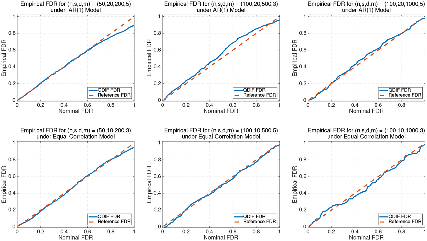
Empirical FDR of the proposed method in AR(1) and equal correlation models, where we take the correlation parameter as 0.75.

Finally, we investigate the empirical power of the proposed test, and compare it with some other high-dimensional inference procedures: the debiased Lasso method (Zhang and Zhang, 2014; van de Geer et al., 2014) and the decorrelation method (Ning and Liu, 2017) by pretending all observations are independent. In particular, we test H₀ : β₁ = 0, under the Dirac setting, where the signal of β₁ gradually increase from 0 to 0.7, and we investigate the empirical rejection rate for different settings. The results are summarized in Figure 2. As expected, our QDIF approach achieves better empirical power, especially when the signal is weak and s is relatively large. This is in line with our theoretical results.

Fig 2:

Empirical power for quadratic decorrelated inference (QDIF), debiased Lasso and decorrelation methods under AR(1) and equal correlation models, where we take the correlation parameter as 0.75.

4.2. BMI dataset.

We further evaluate our method using a BMI genomic dataset from the Framingham Heart Study (FHS). This is a long-term, ongoing cardiovascular study beginning in 1948 under the direction of the National Heart, Lung and Blood institute (NHLBI) on residents of the town of Framingham, Massachusetts. The objective is to identify the important characteristics that contribute to cardiovascular disease. We refer to Jaquish (2007) for more details of the study. Recently, 913,854 SNPs from 24 chromosomes have been genotyped from the Offspring Cohort study. We investigate the issue of obesity as the body mass index (BMI), where BMI = weight(kg)/height(m)². Our dataset contains BMI of 977 samples, where each sample’s BMI value is collected at 26 times. Since there are some missing values presented in the response of different samples, we first adopt n = 234 samples with time points m_i’s ranging from 3 to 7 where their BMI values are recorded. The nonrare SNPs genotypes from the twenty three chromosomes are also recorded. Taking the BMI values as response variables Y, we first screen the features by regressing the BMI values on each of the SNPs, and only keep the SNPs with marginal P-value less than 0.05. This reduces the dimension to d = 4,294. Then, for the jth SNP we treat this covariate as Z in Section 2 and the rest of the covariates as U. We apply the proposed QDIF method to test whether the jth SNP is associated with BMI, where we use the same basis matrices as in the simulations. The obtained p-value is recorded as P_j as in Section 3. We repeat this procedure for all the SNPs, which yields a sequence of p-values P₁, …, P_d. When we select important SNPs based on these p-values, we need to account for the fact that we have been looking at a large number of candidate SNPs (the so called multiple testing effect). Failure to account for the multiple testing effect causes irreproducibility of the results and may yield misleading scientific conclusions. Given the practical importance of this problem, we developed a rigorous result on the FDR control. Applying our result to the data analysis, we find that the 12289th position of the 1st chromosome, 681st, 756th and 19880th SNPs of the 10th chromosome, and 1189th and 12075th SNPs of the 20th chromosome are the significant SNPs under the FDR at 10%. Interestingly, it is known that the 10th and 20th chromosomes are related to the obesity (Dong et al., 2003), which matches our results that the significant SNPs are mostly located at the 10th and 20th chromosomes.

5. Technical Lemmas and Proofs.

5.1. Technical lemmas.

In this subsection, we provide some technical lemmas used in our proofs in Sections 2 and 3. The proofs of these technical lemmas are given in the supplementary material Fang et al. (2018).

The first lemma on the rate of convergence of random matrices in the spectral norm is derived from the matrix Bernsteins inequality and is fundamental for the rest of the proof.

Lemma 5.1. Suppose that Assumptions 2.1 – 2.5 and $\frac{d_0{(\text{log }n)}^2\text{log }{d}_0}{n}=o\text{(1)}$ hold. Then

$$\begin{gathered} \underset{1\le k\le K}{\text{max}}{\Vert \nabla {\overline{S}}_k^{*}\left({\theta }^{*}\right)-g_{0k}\left({\theta }^{*}\right)\Vert }_2={\mathcal{O}}_{\mathbb{P}}(\sqrt{d_0\text{log}{d}_0/n}), \\ \underset{1\le k\le K}{\text{max}}{\Vert \frac{1}{n}\sum _{i=1}^n{\left(Z_i-U_i{W}_k^{*}\right)}^T{\Psi }_i\left(Z_i-U_i{W}_k^{*}\right)-g_{0k}\left({\theta }^{*}\right)\Vert }_2={\mathcal{O}}_{\mathbb{P}}(\sqrt{d_0\text{log}{d}_0/n}), \\ \underset{1\le k\le K}{\text{max}}{\Vert \frac{1}{n}\sum _{i=1}^n{Z}_i{\Psi }_i{Z}_i-\mathbb{E}\left(Z_i{\Psi }_i{Z}_i\right)\Vert }_2={\mathcal{O}}_{\mathbb{P}}(\sqrt{d_0\text{log}{d}_0/n}), \end{gathered}$$ (5.1)

and

$${\Vert \frac{1}{n}\sum _{i=1}^n{S}_i^{*}\left({\mathit{\theta }}^{*}\right)S_i^{*T}\left({\mathit{\theta }}^k\right)-C^{*}\Vert }_2={\mathcal{O}}_{\mathbb{P}}(\sqrt{d_0\text{log }{d}_0{(\text{log }n)}^2/n}).$$ (5.2)

Lemma 5.2. Recall that $\widehat{\mathbf{g}}(\mathit{\theta })=\nabla {\overline{S}}_n(\mathit{\theta })$ and ${\mathbf{g}}_0(\mathit{\theta })=\mathbb{E}\left\{\nabla S_i^{*}(\mathit{\theta })\right\}$. Under the conditions in Theorem 2.7, we have

$${\Vert \widehat{g}(\widehat{\theta })-g_0\left({\theta }^{*}\right)\Vert }_2={\mathcal{O}}_{\mathbb{P}}\left(\sqrt{\frac{\left(s\vee s^{\prime }\right)d_0\text{log}d}{n}}\right).$$

$${\Vert \widehat{\mathbf{\text{g}}}\left({\theta }^{*}\right)-{\mathbf{\text{g}}}_0\left({\theta }^{*}\right)\Vert }_2={\mathcal{O}}_{\mathbb{P}}\left(\sqrt{\frac{\left(s\vee s^{\prime }\right)d_0\text{log}d}{n}}\right).$$

Lemma 5.3. Recall that $\widehat{\mathbf{\text{C}}}=n^{-1}\sum _{i=1}^n{\widehat{\text{S}}}_i(\widehat{\mathit{\theta }}){\widehat{\text{S}}}_i^T(\widehat{\mathit{\theta }})$ in (2.9), where ${\widehat{S}}_i(\mathit{\theta })={\left\{{\widehat{S}}_{i1}(\mathit{\theta }),\dots ,{\widehat{S}}_{iK}(\mathit{\theta })\right\}}^T$, and $C^{*}=\mathbb{E}\left\{S_i^{*}\left({\mathit{\theta }}^{*}\right)S_i^{*}{\left({\mathit{\theta }}^{*}\right)}^T\right\}$ in (2.16), where ${\text{S}}_i^{*}\left({\mathit{\theta }}^{*}\right)={\left(S_{i1}^{*}\left({\mathit{\theta }}^{*}\right),\dots ,S_{iK}^{*}\left({\mathit{\theta }}^{*}\right)\right)}^T$. Under the conditions in Theorem 2.7, we have

$${\Vert \widehat{C}-C^{*}\Vert }_2={\mathcal{O}}_{\mathbb{P}}\left(\sqrt{\frac{d_0\left(s\vee s^{\prime }\right)\text{log }d{(\text{log }n)}^2}{n}}\right).$$

Lemma 5.4. Under the same conditions as in Theorem 2.7, we have,

$$\underset{1\le k\le K}{\text{max}}{\Vert {\overline{S}}_{nk}\left({\mathit{\theta }}^{*}\right)-\frac{1}{n}\sum _{i=1}^n{S}_{ik}^{*}\left({\mathit{\theta }}^{*}\right)\Vert }_2={\mathcal{O}}_{\mathbb{P}}\left(\frac{d_0^{1/2}\left(s\vee s^{\prime }\right)\text{ log }d\text{ log }n}{n}\right).$$

Lemma 5.5. Recall that $Q_n^{*}(\mathit{\theta })={\overline{S}}_n^{*}{(\mathit{\theta })}^T{C}^{*-1}{\overline{S}}_n^{*}(\mathit{\theta })$, where ${\overline{S}}^{*}(\mathit{\theta })=\frac{1}{n}\sum _{i=1}^n{S}_i^{*}(\mathit{\theta })$. Under the same conditions as in Theorem 2.7, we have

$${\Vert \nabla Q_n^{*}\left({\mathit{\theta }}^{*}\right)\Vert }_2={\mathcal{O}}_{\mathbb{P}}\left(\sqrt{\frac{d_0}{n}}\right),$$

$${\Vert \nabla {\tilde{Q}}_n\left({\mathit{\theta }}^{*}\right)-\nabla Q_n^{*}\left({\mathit{\theta }}^{*}\right)\Vert }_2={\mathcal{O}}_{\mathbb{P}}\left(\frac{d_0{\left\{\left(s\vee s^{\prime }\right)\text{log }d{(\text{log }n)}^2\right\}}^{1/2}}{n}+\frac{d_0^{1/2}\left(s\vee s^{\prime }\right)\text{log }d\text{log }n}{n}\right).$$

Lemma 5.6. Let c be a small constant. Under the conditions in Theorem 2.7, uniformly over ${\Vert \mathit{\theta }-{\mathit{\theta }}^{*}\Vert }_2\le c{d}_0^{-1/2}$ it holds that with probability tending to one

$${\tilde{Q}}_n(\mathit{\theta })-{\tilde{Q}}_n\left({\mathit{\theta }}^{*}\right)-\nabla {\tilde{Q}}_n\left({\mathit{\theta }}^{*}\right)\left(\mathit{\theta }-{\mathit{\theta }}^{*}\right)\ge C{\Vert \mathit{\theta }-{\mathit{\theta }}^{*}\Vert }_2^2$$

for some positive constant C.

Lemma 5.7. Suppose Assumptions 2.1, 2.2, 2.3, 2.4 and 2.5 hold for all ${\mathit{\beta }}_j^{*}$ for j ∈ [d], and suppose that $\lambda \asymp {\lambda }^{\prime }\asymp \sqrt{n^{-1}}\text{log }d$ and n^−1/2s(log d)(log n) = o(1/log d). Let the “ideal” version of ${\tilde{\mathit{\beta }}}_j$ be

$$\frac{1}{n}\sum _{i=1}^n{A}_{ij}=\frac{1}{n}\sum _{i=1}^n{\left\{{\mathbf{\text{g}}}_{0j}\left({\mathit{\beta }}_j^{*}\right){\mathbf{\text{C}}}_j^{*-1}{\mathbf{\text{g}}}_{0j}\left({\mathit{\beta }}_j^{*}\right)\right\}}^{-1}{\mathbf{\text{g}}}_{0j}\left({\mathit{\beta }}_j^{*}\right){\mathbf{\text{C}}}_j^{*-1}\cdot {\text{S}}_{ij}^{*}\left({\mathit{\beta }}_j^{*}\right),$$ (5.3)

where ${\mathbf{g}}_{0j}^{*}$, $C_j^{*}$ and $S_{ij}^{*}\left({\mathit{\beta }}_j^{*}\right)$ denote corresponding g₀, C* and $S_i^{*}\left({\mathit{\beta }}_j^{*}\right)$ in the previous section for ${\mathit{\beta }}_j^{*}$, and let the ideal version of ${\widehat{T}}_j$ be

$$T_j=\sqrt{n}{\sigma }_j^{-1}\left(\frac{1}{n}\sum _{i=1}^n{A}_{ij}\right),$$

where σ_j is defined in (2.21). We have that $\sqrt{n}{\tilde{\mathit{\beta }}}_j$ converges to $\frac{1}{\sqrt{n}}\sum _{i=1}^n{A}_{ij}$ such that as n → ∞,

$$\underset{j\in {\mathcal{H}}_0}{\text{max}}\left|\sqrt{n}{\tilde{\mathit{\beta }}}_j-\frac{1}{\sqrt{n}}\sum _{i=1}^n{A}_{ij}\right|={\mathcal{O}}_{\mathbb{P}}\left(n^{-1/2}s(\text{log }d)(\text{log }n)\right),$$

and

$$\underset{j}{\text{max}}|{\widehat{T}}_j-T_j|={\mathcal{O}}_{\mathbb{P}}\left(n^{-1/2}s(\text{log }d)(\text{log }n)\right).$$

Lemma 5.8. Suppose the conditions in Theorem 3.1 holds. Let r_d be any sequence such that r_d → ∞ as d → ∞, and $r_d=o\left(|{\mathcal{S}}_1|\right)$. Then we have

$$\underset{r_d/d\le u\le 1}{\text{sup}}\left|\frac{\sum _{j\in {\mathcal{S}}_0}1\left\{P_j\le u\right\}}{u\cdot |{\mathcal{S}}_0|}-1\right|\to 0,$$

in probability.

5.2. Proof of main results.

Proof of Theorem 2.7. Since ${\mathit{\theta }}^{*}-{\widehat{\mathit{\theta }}}_2\lesssim \sqrt{s\text{log }d/n}\le c{d}_0^{-1/2}$ under condition (2.18), we claim that θ* lies in Θ_n with probability tending to one. By the definition of $\tilde{\mathit{\theta }}$, it holds that ${\tilde{Q}}_n(\tilde{\mathit{\theta }})\le {\tilde{Q}}_n\left({\mathit{\theta }}^{*}\right)$, which further implies

$${\tilde{Q}}_n(\tilde{\mathit{\theta }})-{\tilde{Q}}_n\left({\mathit{\theta }}^{*}\right)-\nabla {\tilde{Q}}_n\left({\mathit{\theta }}^{*}\right)\left(\tilde{\mathit{\theta }}-{\mathit{\theta }}^{*}\right)\le -\nabla {\tilde{Q}}_n\left({\mathit{\theta }}^{*}\right)\left(\tilde{\mathit{\theta }}-{\mathit{\theta }}^{*}\right).$$

By Lemma 5.6, the left hand side is lower bounded by $C{\Vert \tilde{\mathit{\theta }}-{\mathit{\theta }}^{*}\Vert }_2^2$. Thus, by Cauchy-Schwartz inequality,

$$C{\Vert \tilde{\mathit{\theta }}-{\mathit{\theta }}^{*}\Vert }_2^2\le {\Vert \nabla {\tilde{Q}}_n\left({\mathit{\theta }}^{*}\right)\Vert }_2{\Vert \tilde{\mathit{\theta }}-{\mathit{\theta }}^{*}\Vert }_2\le \left(\nabla {\Vert {\tilde{Q}}_n\left({\mathit{\theta }}^{*}\right)-\nabla Q_n^{*}\left({\mathit{\theta }}^{*}\right)\Vert }_2+{\Vert \nabla Q_n^{*}\left({\mathit{\theta }}^{*}\right)\Vert }_2\right){\Vert \tilde{\mathit{\theta }}-{\mathit{\theta }}^{*}\Vert }_2.$$

Together with Lemma 5.5, we have ${\Vert \tilde{\mathit{\theta }}-{\mathit{\theta }}^{*}\Vert }_2={\mathcal{O}}_{\mathbb{P}}(\sqrt{d_0/n})$, which completes the proof.

Proof of Theorem 2.8. We first note that

$$\Vert \tilde{\mathit{\theta }}-\widehat{\mathit{\theta }}{\Vert }_2\le {\Vert \tilde{\mathit{\theta }}-{\mathit{\theta }}^{*}\Vert }_2+{\Vert \widehat{\mathit{\theta }}-{\mathit{\theta }}^{*}\Vert }_2\lesssim \sqrt{\frac{d_0}{n}}+\sqrt{\frac{s\text{log }d}{n}}=o_{\mathbb{P}}\left(\frac{1}{\sqrt{d_0}}\right).$$

This implies $\tilde{\mathit{\theta }}$ belongs to the interior of Θ_n. By the first order optimality condition, $\tilde{\mathit{\theta }}$ satisfies

$$\widehat{\mathbf{g}}{(\tilde{\mathit{\theta }})}^T{\widehat{C}}^{-1}{\overline{S}}_n(\tilde{\mathit{\theta }})=0,\text{ where }\widehat{\mathbf{g}}(\mathit{\theta })=\partial {\overline{S}}_n(\mathit{\theta })/\partial \mathit{\theta }.$$

By the mean-value theorem for vector valued functions, for each component of ${\overline{S}}_n(\tilde{\mathit{\theta }})$, say ${\left({\overline{S}}_n(\tilde{\mathit{\theta }})\right)}_j$ there exists ${\overline{\mathit{\theta }}}_j={\zeta }_j{\mathit{\theta }}^{*}+\left(1-{\zeta }_j\right)\tilde{\mathit{\theta }}$ for some ζ_j ∈ [0, 1] such that ${\left({\overline{S}}_n(\tilde{\mathit{\theta }})-{\overline{S}}_n\left({\mathit{\theta }}^{*}\right)\right)}_j={\left[\partial {\left({\overline{S}}_n\left({\overline{\mathit{\theta }}}_j\right)\right)}_j/\partial \mathit{\theta }\right]}^T\left(\tilde{\mathit{\theta }}-{\mathit{\theta }}^{*}\right)$. For notational simplicity, we suppress the subscript j in ${\overline{\mathit{\theta }}}_j$, and write it as

$$\widehat{\mathbf{g}}{(\tilde{\mathit{\theta }})}^T{\widehat{C}}^{-1}\left\{{\overline{S}}_n\left({\mathit{\theta }}^{*}\right)+\widehat{\mathbf{g}}{(\overline{\mathit{\theta }})}^T\left(\tilde{\mathit{\theta }}-{\mathit{\theta }}^{*}\right)\right\}=0.$$

Thus, we have

$$\left\{\widehat{\mathbf{\text{g}}}{(\tilde{\mathit{\theta }})}^T{\widehat{C}}^{-1}\widehat{\mathbf{\text{g}}}(\overline{\mathit{\theta }})\right\}\left(\tilde{\mathit{\theta }}-{\mathit{\theta }}^{*}\right)=-\widehat{\mathbf{\text{g}}}{(\tilde{\mathit{\theta }})}^T{\widehat{C}}^{-1}{\overline{S}}_n\left({\mathit{\theta }}^{*}\right).$$

Define

$$T_1=\left[{\left\{\widehat{\mathbf{\text{g}}}{(\tilde{\mathit{\theta }})}^T{\widehat{\mathbf{\text{C}}}}^{-1}\widehat{\mathbf{\text{g}}}(\overline{\mathit{\theta }})\right\}}^{-1}-{\left\{{\mathbf{\text{g}}}_0{\left({\mathit{\theta }}^{*}\right)}^T{\mathbf{\text{C}}}^{*-1}{\mathbf{\text{g}}}_0\left({\mathit{\theta }}^{*}\right)\right\}}^{-1}\right]\cdot \widehat{\mathbf{\text{g}}}{(\tilde{\mathit{\theta }})}^T{\widehat{\mathbf{\text{C}}}}^{-1}{\overline{\text{S}}}_n\left({\mathit{\theta }}^{*}\right),$$

$$T_2={\left\{{\mathbf{\text{g}}}_0{\left({\mathit{\theta }}^{*}\right)}^T{\mathbf{\text{C}}}^{*-1}{\mathbf{\text{g}}}_0\left({\mathit{\theta }}^{*}\right)\right\}}^{-1}\left\{\widehat{\mathbf{\text{g}}}{(\tilde{\mathit{\theta }})}^T{\widehat{\mathbf{\text{C}}}}^{-1}{\overline{\text{S}}}_n\left({\mathit{\theta }}^{*}\right)-{\mathbf{\text{g}}}_0{\left({\mathit{\theta }}^{*}\right)}^T{\mathbf{\text{C}}}^{*-1}\cdot \frac{1}{n}\sum _{i=1}^n{\text{S}}_i^{*}\left({\mathit{\theta }}^{*}\right)\right\}.$$

$$\overline{\xi }=\frac{1}{n}\sum _{i=1}^n{\xi }_i,\text{ where }{\xi }_i=-{\left\{{\mathbf{\text{g}}}_0{\left({\mathit{\theta }}^{*}\right)}^T{\mathbf{\text{C}}}^{*-1}{\mathbf{\text{g}}}_0\left({\mathit{\theta }}^{*}\right)\right\}}^{-1}{\mathbf{\text{g}}}_0{\left({\mathit{\theta }}^{*}\right)}^T{\mathbf{\text{C}}}^{*-1}{\text{S}}_i^{*}\left({\mathit{\theta }}^{*}\right).$$

Then, it holds that $\tilde{\mathit{\theta }}-{\mathit{\theta }}^{*}=-T_1-T_2+\overline{\xi }$. Putting together Lemmas 5.2, 5.3 and 5.4, we can show that

$${\Vert T_1\Vert }_2={\mathcal{O}}_{\mathbb{P}}\left(\frac{d_0^{3/2}}{n}+\frac{d_0{\left\{\left(s\vee s^{\prime }\right)\text{log }d{(\text{log }n)}^2\right\}}^{1/2}}{n}\right)$$

with some tedious algebraic manipulation similar to the proof of Lemma 5.6. In addition, we can show that

$${\Vert T_2\Vert }_2={\mathcal{O}}_{\mathbb{P}}\left(\frac{d_0^{3/2}}{n}+\frac{d_0{\left\{\left(s\vee s^{\prime }\right)\text{log }d{(\text{log }n)}^2\right\}}^{1/2}}{n}+\frac{d_0^{1/2}\left(s\vee s^{\prime }\right)\text{log }d\text{log }n}{n}\right).$$

Combining the above results, we have

$${\Vert \tilde{\mathit{\theta }}-{\mathit{\theta }}^{*}-\overline{\mathit{\xi }}\Vert }_2={\mathcal{O}}_{\mathbb{P}}\left(\frac{d_0^{3/2}}{n}+\frac{d_0{\left\{\left(s\vee s^{\prime }\right)\text{log }d{(\text{log }n)}^2\right\}}^{1/2}}{n}+\frac{d_0^{1/2}\left(s\vee s^{\prime }\right)\text{log }d\text{log }n}{n}\right).$$

To show the limiting distribution of $n{(\tilde{\mathit{\theta }}-\mathit{\theta })}^T{\Sigma }_{\mathit{\theta }}^{-1}(\tilde{\mathit{\theta }}-\mathit{\theta })$, we first note that

$$\begin{gathered} d_0^{-1/2}n|{\left(\tilde{\mathit{\theta }}-{\mathit{\theta }}^{*}\right)}^T{\Sigma }_{\mathit{\theta }}^{-1}\left(\tilde{\mathit{\theta }}-{\mathit{\theta }}^{*}\right)-{\overline{\mathit{\xi }}}^T{\Sigma }_{\mathit{\theta }}^{-1}\overline{\mathit{\xi }}| \\ \le d_0^{-1/2}n\left[|{\left(\tilde{\mathit{\theta }}-{\mathit{\theta }}^{*}-\overline{\mathit{\xi }}\right)}^T{\Sigma }_{\mathit{\theta }}^{-1}\left(\tilde{\mathit{\theta }}-{\mathit{\theta }}^{*}\right)|+|{\overline{\mathit{\xi }}}^T{\Sigma }_{\mathit{\theta }}^{-1}\left(\tilde{\mathit{\theta }}-{\mathit{\theta }}^{*}-\overline{\mathit{\xi }}\right)|\right] \\ \le d_0^{-1/2}n\left[{\Vert \tilde{\mathit{\theta }}-{\mathit{\theta }}^{*}-\overline{\mathit{\xi }}\Vert }_2{\Vert {\Sigma }_{\mathit{\theta }}^{-1}\Vert }_2{\Vert \tilde{\mathit{\theta }}-{\mathit{\theta }}^{*}\Vert }_2+\Vert \overline{\mathit{\xi }}{\Vert }_2{\Vert {\Sigma }_{\mathit{\theta }}^{-1}\Vert }_2{\Vert \tilde{\mathit{\theta }}-{\mathit{\theta }}^{*}-\overline{\mathit{\xi }}\Vert }_2\right] \\ \lesssim \frac{n}{d_0^{1/2}}\left[\frac{d_0^{3/2}}{n}+\frac{d_0{\left\{\left(s\vee s^{\prime }\right)\text{log }d{(\text{log }n)}^2\right\}}^{1/2}}{n}+\frac{d_0^{1/2}\left(s\vee s^{\prime }\right)\text{log }d\text{log }n}{n}\right]\frac{d_0^{1/2}}{n^{1/2}}=o_{\mathbb{P}}(1), \end{gathered}$$

by Theorem 2.7 and the assumed conditions. Thus, it suffices to show the limiting distribution of ${\overline{\mathit{\xi }}}^T{\Sigma }_{\mathit{\theta }}^{-1}\overline{\mathit{\xi }}$. Note that $\mathbb{E}{\Vert {\Sigma }_{\mathit{\theta }}^{-1/2}{\mathit{\xi }}_i\Vert }_2^3\lesssim \mathbb{E}{\Vert S_i^{*}\left({\mathit{\theta }}^{*}\right)\Vert }_2^3\lesssim d_0^{3/2}$. Theorem 1.1 in Bentkus (2003) implies

$$\underset{B\in \mathcal{B}}{\text{sup}}\left|\mathbb{P}\left(\frac{1}{n^{1/2}}\sum _{i=1}^n{\Sigma }_{\mathit{\theta }}^{-1/2}{\mathit{\xi }}_i\in B\right)-\mathbb{P}(N\in B)\right|\le \frac{C{d}_0^{3/2}}{n^{1/2}},$$

where $\mathcal{B}$ is the set of all Euclidean balls in ${ℝ}^{d_0}$, C is a positive constant and $N=\left(N_1,\dots ,N_{d_0}\right)$ are d₀ independent N(0, 1). Finally, we obtain for any $t\in ℝ$,

$$\begin{gathered} \mathbb{P}\left(\frac{n{\overline{\mathit{\xi }}}^T{\Sigma }_{\mathit{\theta }}^{-1}\overline{\mathit{\xi }}-d_0}{\sqrt{2d_0}}\le t\right)\le \mathbb{P}\left(\frac{\Vert N{\Vert }_2^2-d_0}{\sqrt{2d_0}}\le t\right)+\frac{C{d}_0^{3/2}}{n^{1/2}} \\ =\mathbb{P}\left(\frac{1}{\sqrt{d_0}}\sum _{i=1}^{d_0}\frac{N_i^2-1}{\sqrt{2}}\le t\right)+\frac{C{d}_0^{3/2}}{n^{1/2}}\le \Phi (t)+\frac{C^{\prime }}{d_0^{1/2}}+\frac{C{d}_0^{3/2}}{n^{1/2}} \end{gathered}$$

where Φ(·) is the c.d.f. of a standard normal distribution and C′ is a absolute constant from the standard Berry-Esseen bound. The same probability can be lower bounded by using the same argument. Thus, as d₀, n→ ∞, $\left(n{\overline{\mathit{\xi }}}^T{\Sigma }_{\mathit{\theta }}^{-1}\overline{\mathit{\xi }}-d_0\right)/\sqrt{2d_0}$ converges weakly to N(0, 1). When d₀ is fixed, the Layponov condition for $\frac{1}{n}\sum _{i=1}^n{v}^T{\mathit{\xi }}_i$ holds for any $v\in {ℝ}^{d_0}$ and thus $\frac{1}{n^{1/2}}\sum _{i=1}^n{v}^T{\mathit{\xi }}_i\to N\left(0,v^T{\Sigma }_{\mathit{\theta }}v\right)$. Finally, we obtain (2.22) by applying the Cramer-Wald device.

Proof of Theorem 3.1. For notational simplicity, we suppress the dependence of ${\widehat{u}}_{\alpha ,t}$ on t. By the definition of FDP(u) and ${\widehat{\text{FDP}}}_t(u)$, we have

$$\text{FDP}\left({\widehat{u}}_{\alpha }\right)={\widehat{\text{FDP}}}_{\lambda }\left({\widehat{u}}_{\alpha }\right)\cdot \frac{|{\mathcal{S}}_0|}{\pi (t)d}\cdot \frac{\sum _{j\in {\mathcal{S}}_0}\mathbb{1}\left\{P_j\le {\widehat{u}}_{\alpha }\right\}}{{\widehat{u}}_{\alpha }\cdot |{\mathcal{S}}_0|}.$$ (5.5)

We first show that ${\left(u\cdot |{\mathcal{S}}_0|\right)}^{-1}\sum _{j\in {\mathcal{S}}_0}\mathbb{1}\left\{P_j\le u\right\}\to 1$ in probability. We prove a moderate deviation result for this quantity. By assumption, we have $|{\mathcal{S}}_1|\to \infty$. Let r_d be a sequence such that r_d → ∞ as d → ∞, and $r_d=o\left(|{\mathcal{S}}_1|\right)$. We first prove that $\mathbb{P}\left({\widehat{u}}_{\alpha }\le r_d/d\right)\to 0$ as n → ∞. Note that

$$1-{\chi }_1^2(2\text{log }d)=2(1-\Phi (\sqrt{2\text{log }d}))\le \sqrt{2/\pi }{(d\sqrt{2\text{log }d})}^{-1}\lesssim r_d/d.$$

Hence, for any $j\in {\mathcal{S}}_1$, we have

$$\mathbb{P}\left(P_j\le r_d/d\right)=\mathbb{P}\left({\Lambda }_{nj}\ge 1-{\chi }_1^{-2}\left(r_d/d\right)\right)\ge \mathbb{P}\left({\Lambda }_{nj}\ge 2\text{log }d\right).$$ (5.6)

Recall that $V_{nj}:=\sqrt{n}\left({\tilde{\mathit{\beta }}}_j-{\mathit{\beta }}_j^{*}\right)/\widehat{\sigma }$. By extending the proof of Theorem 2.8, we get

$$\underset{n\to \infty }{\text{lim}}\underset{j\in \left\{1,\dots ,d\right\}}{\text{max}}\underset{x\in ℝ}{\text{sup}}|\mathbb{P}\left(V_{nj}\le x\right)-\Phi (x)|=0.$$ (5.7)

For any $j\in {\mathcal{S}}_1$, we have

$${\Lambda }_{nj}=n{\widehat{\mathit{\beta }}}_j^2/{\widehat{\sigma }}^2={\left\{V_{nj}+\sqrt{n}{\mathit{\beta }}_j^{*}/\widehat{\sigma }\right\}}^2.$$

Therefore, we have that

$$\begin{gathered} \mathbb{P}\left({\Lambda }_{nj}\le 2\text{log }d\right)\le \mathbb{P}\left(|V_{nj}+\sqrt{n}{\mathit{\beta }}_j^{*}/\widehat{\sigma }|\le \sqrt{2\text{log }d}\right) \\ \le \mathbb{P}\left(-|V_{nj}|+\sqrt{n}|{\mathit{\beta }}_j^{*}|/\widehat{\sigma }\le \sqrt{2\text{log }d}\right)***\le \mathbb{P}\left(C{C}^{\prime }\sqrt{\text{log }d}-{(\text{log }d)}^{1/4}\le \sqrt{2\text{log }d}\right)+\mathbb{P}\left(|V_{nj}|\ge {(\text{log }d)}^{1/4}\right). \end{gathered}$$

where in the last inequality we used the condition that $|{\mathit{\beta }}_j^{*}|\ge C\sqrt{(\text{log }d)/n}$ for $j\in {\mathcal{S}}_1$ and $1/\widehat{\sigma }\ge C^{\prime }$. If $C{C}^{\prime }>\sqrt{3}$, hence $C{C}^{\prime }\sqrt{\text{log }d}-{(\text{log }d)}^{1/4}>\sqrt{2\text{log }d}$ for large enough d. Moreover, by (5.7)

$$\begin{gathered} \underset{j\in {\mathcal{S}}_1}{\text{max}}\mathbb{P}\left(|V_{nj}|\ge {(\text{log }d)}^{1/4}\right) \\ \le \underset{j\in {\mathcal{S}}_1}{\text{max}}\left|\mathbb{P}\left(|V_{nj}|\ge {(\text{log }d)}^{1/4}\right)-2\left\{1-\Phi \left({(\text{log }d)}^{1/4}\right)\right\}\right|+2\left\{1-\Phi \left({(\text{log }d)}^{1/4}\right)\right\}\to 0. \end{gathered}$$

Hence we get ${\text{max}}_{j\in {\mathcal{S}}_1}\mathbb{P}\left({\Lambda }_{nj}\le 2\text{log }d\right)\to 0$. Therefore, by (5.6), we conclude that $\mathbb{P}\left(P_j\le r_d/d\right)\to 1$, uniformly over $j\in {\mathcal{S}}_1$. Therefore, we have

$$\frac{1}{|{\mathcal{S}}_1|}\sum _{j\in {\mathcal{S}}_1}\mathbb{P}\left(P_j\le \frac{r_d}{d}\right)\to 1,$$

which implies that $1/|{\mathcal{S}}_1|\sum _{j\in {\mathcal{S}}_1}\mathbb{1}\left\{P_j\le r_d/d\right\}\to 1$ in L₁ and in probability. Hence, we have

$${\widehat{\text{FDP}}}_t\left(r_d/d\right)=\frac{\pi (t)\cdot r_d}{\sum _{j=1}^d\mathbb{1}\left\{P_j\le r_d/d\right\}}\le \pi (t)\cdot \frac{|{\mathcal{S}}_1|}{\sum _{j\in {\mathcal{S}}_1}\mathbb{1}\left\{P_j\le r_d/d\right\}}\cdot \frac{r_d}{|{\mathcal{S}}_1|}.$$

As $r_d=o\left(|{\mathcal{S}}_1|\right)$, we conclude that ${\widehat{\text{FDP}}}_t\left(r_d/d\right)\to 0<\alpha$ in probability, and hence by the definition of ${\widehat{u}}_{\alpha }$, we obtain

$$\mathbb{P}\left({\widehat{u}}_{\alpha }\ge r_d/d\right)\to 1.$$ (5.8)

Hence, by (5.8) and Lemma 5.8, we conclude that ${\left({\widehat{u}}_{\alpha }\cdot |{\mathcal{S}}_0|\right)}^{-1}\sum _{j\in {\mathcal{S}}_0}1\left\{P_j\le {\widehat{u}}_{\alpha }\right\}\to 1$ in probability. Finally, by the definition of π(t), we have

$$\frac{|{\mathcal{S}}_0|}{\pi (t)d}=\frac{|{\mathcal{S}}_0|}{\text{min}\left(\sum _{j=1}^d\mathbb{1}\left\{P_j\ge t\right\}/(1-t),d\right)}.$$

If $\sum _{j=1}^d\mathbb{1}\left\{P_j\ge t\right\}/(1-t)\le d$ we have

$$\frac{|{\mathcal{S}}_0|}{\pi (t)d}=\frac{|{\mathcal{S}}_0|(1-t)}{d-\sum _{j=1}^d\mathbb{1}\left\{P_j\le t\right\}}=\frac{|{\mathcal{S}}_0|(1-t)}{d-\left(\sum _{j\in {\mathcal{S}}_0}+\sum _{j\notin {\mathcal{S}}_0}\right)\mathbb{1}\left\{P_j\le t\right\}}.$$

We have $|{\mathcal{S}}_0|/d\to 1$, and $\left(1/|{\mathcal{S}}_0|\right)\sum _{j\notin {\mathbb{S}}_0}\mathbb{1}\left\{P_j\le t\right\}\le \left(d-|{\mathcal{S}}_0|\right)/|{\mathcal{S}}_0|\to 0$ in probability. Moreover, given any t ∈ [c, 1), for d large enough, we have t ≥ r_d/d. Hence by Lemma (5.8), we have $\left(1/|{\mathcal{S}}_0|\right)\sum _{j\in {\mathcal{S}}_0}\mathbb{1}\left\{P_j\le t\right\}\to t$ in probability. Hence we conclude that $|{\mathcal{S}}_0|/\left(\pi \left(t\right)\cdot d\right)\to 1$ in probability. On the other hand, if $\sum _{j=1}^d\mathbb{1}\left\{P_j\ge t\right\}/(1-t)>d$, we have $|{\mathcal{S}}_0|/(\pi (t)\cdot d)=|{\mathcal{S}}_0|/d\to 1$.

Putting together the above results and by (5.5), we get $\text{FDP}\left({\widehat{u}}_{\alpha }\right)\le \alpha$ and similarly $\text{FDR}\left({\widehat{u}}_{\alpha }\right)\le \alpha$ in probability, hence concluding the proof.