MIDCAN: A multiple input deep convolutional attention network for Covid-19 diagnosis based on chest CT and chest X-ray

Abstract

Background

COVID-19 has caused 3.34m deaths till 13/May/2021. It is now still causing confirmed cases and ongoing deaths every day.

Method

This study investigated whether fusing chest CT with chest X-ray can help improve the AI's diagnosis performance. Data harmonization is employed to make a homogeneous dataset. We create an end-to-end multiple-input deep convolutional attention network (MIDCAN) by using the convolutional block attention module (CBAM). One input of our model receives 3D chest CT image, and other input receives 2D X-ray image. Besides, multiple-way data augmentation is used to generate fake data on training set. Grad-CAM is used to give explainable heatmap.

Results

The proposed MIDCAN achieves a sensitivity of 98.10±1.88%, a specificity of 97.95±2.26%, and an accuracy of 98.02±1.35%.

Conclusion

Our MIDCAN method provides better results than 8 state-of-the-art approaches. We demonstrate the using multiple modalities can achieve better results than individual modality. Also, we demonstrate that CBAM can help improve the diagnosis performance.

1. Introduction

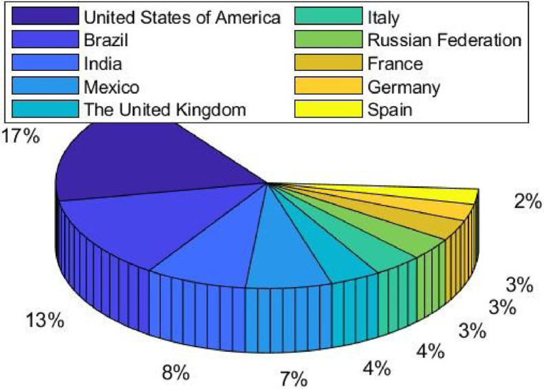
COVID-19 (also known as coronavirus) pandemic is an ongoing infectious disease caused by severe acute respiratory syndrome (SARS) coronavirus 2 [1]. As of 13/May/2021, there are over 161.14m confirmed cases and over 3.34m deaths attributed to COVID-19. The cumulative deaths of the top 10 countries are shown in Fig. 1 .

Fig. 1.

Top 10 countries in terms of cumulative deaths (13/May/2021).

The main symptoms of COVID-19 are a low fever, a new and ongoing cough, a loss or change to taste and smell. In UK, the vaccines approved were developed by Pfizer/BioNTech, Oxford/AstraZeneca, and Moderna. The joint committee on vaccination and immunization (JCVI) [2] determines the order in which people will be offered the vaccine. At April/2021, people aged 50 and over, people of clinically (extremely) vulnerable, people living or working in the care homes, and health care providers, people with a learning disability are being offered.

Two COVID-19 diagnosis methods are available. The first method is viral testing to test the existence of viral RNA fragments [3]. The shortcomings of swab test [4] are two folds: (i) the swab samples may be contaminated and (ii) it needs to wait from several hours to several days to get the results. The other method is chest imaging. There are two main different chest imaging available: chest computed tomography (CCT) and chest X-ray (CXR)

CCT is one of the best chest imaging techniques so far, because it provides the finest resolution and it is capable of recognizing extremely small nodules [5]. It provides high-quality volumetric 3D chest data. On the other hand, CXR performs poor on soft tissue contrast, and it only provides 2D image [6].

In this paper, we aim to fuse CCT and CXR images, and expects the fusion can improve the performance compared to using CCT or CXR individually. Besides, we create a novel multiple input deep convolutional attention network (MIDCAN) that can handle CCT and CXR images simultaneously, and present the diagnosis output. The contributions of this study are itemized briefly as following five points:

• •Attention mechanism, convolutional block attention module, is included in the proposed MIDCAN model to improve the performance;
• •The proposed MIDCAN model can handle CCT and CXR images simultaneously;
• •Multiple-way data augmentation is employed to overcome overfitting problem;
• •This proposed MIDCAN model gives more accurate performances than individual modality-based approaches;
• •The proposed MIDCAN model is superior to state-of-the-art COVID-19 diagnosis approaches.

2. Literature survey

From previous year, AI field has investigated ongoing researches on automatic COVID-19 diagnosis, which can save the workloads of manual labelling.

For the CCT image based COVID-19 diagnosis, Chen (2020) [7] employed gray-level occurrence matrix (GLCM) as feature extraction method. The authors then used support vector machine (SVM) as the classifier. Yao (2020) [8] combined wavelet entropy (WE) and biogeography-based optimization (BBO). Wu (2020) [9] presented a novel method—wavelet Renyi entropy (WRE) to help diagnose COVID-19. El-kenawy, Ibrahim (2020) [10] proposed a feature selection voting classifier (FSVC) approach for COVID-19 classification. Satapathy (2021) [11] combined DenseNet with optimization of transfer learning setting (OTLS). Saood and Hatem (2021) [12] explored two structurally-different deep learning (DL) methods—U-Net and SegNet—for COVID-19 CT image segmentation.

On the other side, there are several successful AI models for CXR image based COVID-19 diagnosis. For example, Ismael and Sengur (2020) [13] presented a multi-resolution analysis (MRA) approach. Loey, Smarandache (2020) [14] combined generative adversarial network (GAN) with GoogleNet. Their method is abbreviated as GG. Togacar, Ergen (2020) [15] employed social mimic optimization (SMO) for feature selection and combination. Das, Ghosh (2021) [16] used weighted average ensembling technique with convolutional neural network (CNN) for automatic COVID-19 detection.

The main shortcomings of above approaches are three points: (i) They only consider individual modality, either CCT or CXR. (ii) Their AI models are either traditional feature extraction plus classifier model, or modern deep neural network models. Nevertheless, their models lack attention mechanism. (iii) Efficient measures to resist overfitting are missing.

To solve or alleviate above three shortcomings, we proposed the multiple input deep convolutional attention network. The dataset and details of our method will be discussed in Sections 3 and 4, respectively.

3. Dataset

3.1. Data harmonization

This retrospective study was granted to exempt ethical approval. 42 COVID-19 patients and 44 healthy controls (HCs) were recruited. All the data were collected from local hospitals. Each subject $n$ takes a CCT scan a CXR scan, and thus generate a CCT image $A_0\left(n\right)$ and CXR image $B_0\left(n\right)$. Due to different chest sizes of different people and the different sources of scanning machines, the height of image $A_0\left(n\right)$ and the size of $B_0\left(n\right)$ vary.

To make a homogeneous dataset, data harmonization [17] is used. The central 64 slices of CCT image and the central rectangle region of CXR image are reserved. The height and width of CCT slices are resized to $1024\times 1024$, and the CXR image is resized to $2048\times 2048$. They are named $A_1\left(n\right)$ and $B_1\left(n\right)$. We choose 64 and 2048 because we find this can keep the lung part of images while get rid of unrelated body tissues. The details are displayed in Algorithm 1 .

Algorithm 1.

Data harmonization.

Input	CCT image $A_0\left(n\right)$ and CXR image $B_0\left(n\right)$ of subject $n$.
Step 1	For CCT image $A_0\left(n\right)$ 64 central slices are reserved, and top/bottom slices are removed
Step 2	For CXR image $B_0\left(n\right)$ Central rectangle region is reserved, and outskirt pixels are removed.
Step 3	CCT images are resized to $1024\times 1024$, and CXR image is resized to $2048\times 2048$.
Output	CCT image $A_1\left(n\right)$ and CXR image $B_1\left(n\right)$. $size\left[A_1\left(n\right)\right]=1024\times 1024\times 64$. $size\left[B_1\left(n\right)\right]=2048\times 2048$.

3.2. Data Preprocessing

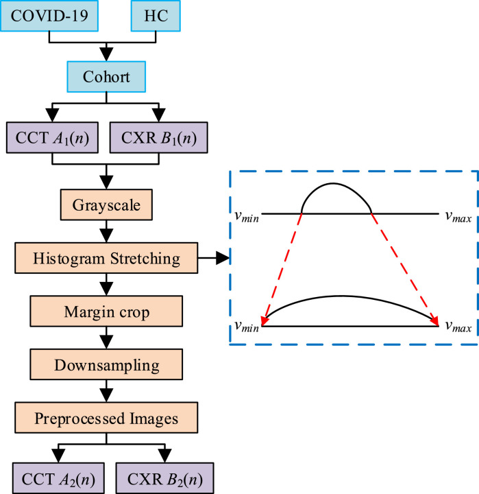
Second, data preprocessing (See Fig. 2 ) is used since both CCT and CXR image contain redundant/unrelated spatial information and their sizes are still too large. First, all the CCT and CXR images are grayscaled. Second, histogram stretch is carried to enhance the image contrast, where $\left(v_{min},v_{max}\right)$ stand for the minimum and maximum grayscale values of our images. Third, the margins at four directions are cropped (e.g., the text in the right side and the check-up bed in bottom side of CCT images, the neck part in the top side of CXR images, the background regions at four directions, etc.). Finally, CCT images are resized to $H^{CCT}\times W^{CCT}\times C^{CCT}$ and CXR images are resized to $H^{CXR}\times W^{CXR}\times 1$.

Fig. 2.

Flowchart of preprocessing.

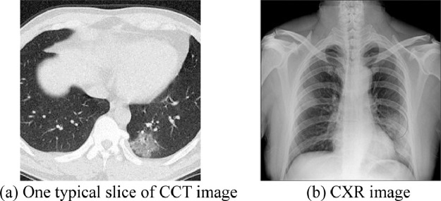
Fig. 3 gives the examples of preprocessed images of a COVID-19 patient. Fig. 3(a) displays one slice out of 16 CCT slices, and Fig. 3(b) displays the CXR image.

Fig. 3.

Pre-processed images of one COVID-19 patient.

4. Methodology

4.1. Convolutional block attention module

Table 1 gives the abbreviation list. DL has gained many successes in prediction/classification quests. Among all the DL structures, convolutional neural network (CNN) [18, 19] is particularly suitable for analyzing 2D/3D images. To help boost the performance of CNN, researches are proposed to modify CNN structures in terms of either depth, or cardinality, or width. Newly, scholars have studied on attention mechanism, and attempted to integrate attention to DL structures. For example, Hu, Shen (2020) [20] proposed squeeze-and-excitation (SE) network. Woo, Park (2018) [21] presented a new convolutional block attention module (CBAM), that improves the traditional convolutional block (CB) by integrating attention mechanism. This study we choose CBAM because CBAM can provider both spatial attention and channel attention, compared to SE.

Table 1.

Abbreviation list.

Meanings	Abbreviations
AM	activation map
AI	artificial intelligence
AP	average pooling
BN	batch normalization
CAM	channel attention module
CCT	chest computed tomography
CXR	chest X-ray
CB	convolutional block
CBAM	convolutional block attention module
CNN	convolutional neural network
DA	data augmentation
DL	deep learning
FMI	Fowlkes–Mallows index
MCC	Matthews correlation coefficient
MP	max pooling
MSD	mean and standard deviation
ReLU	rectified linear unit
SAPN	salt-and-pepper noise
SAM	spatial attention module
SN	speckle noise
SE	squeeze-and-excitation

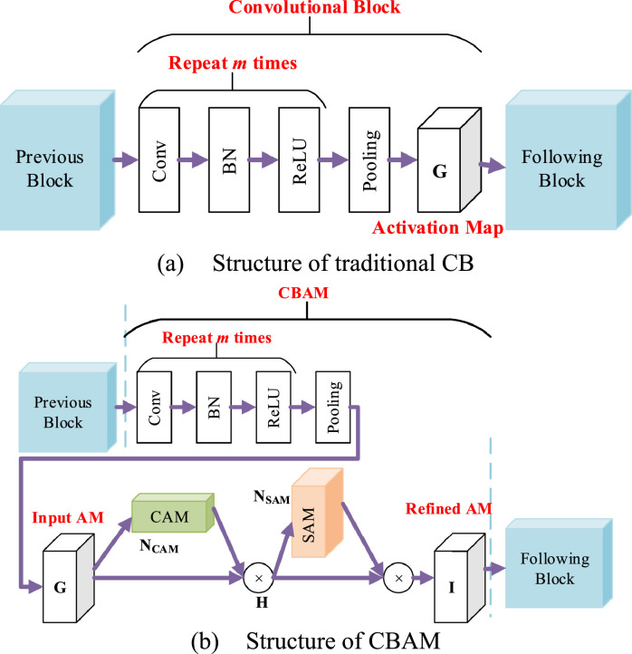
Take a 2D-image input as an example, Fig. 4 (a) displays the structure of a traditional CB. The output of previous block was sent to $m$-repetitions of convolution layer, batch normalization (BN), and rectified linear unit (ReLU) layer. Finally, the $m$-repetitions is followed by a pooling layer. The output is named activation map (AM), symbolized as $\mathbf{G}\in {\mathbb{R}}^{C\times H\times W}$, where $\left(C,H,W\right)$ stands for the sizes of channel, height, and width, respectively.

Fig. 4.

Structural comparison.

In contrast to Fig. 4(a), Fig. 4(b) adds the structure of CBAM, by which two modules: channel attention module (CAM) and spatial attention module (SAM) are added to refine the activation map $\mathbf{G}$. Suppose the CBAM applies a 1D CAM ${\mathbf{N}}_{\mathbf{CAM}}\in {\mathbb{R}}^{C\times 1\times 1}$ and a 2D SAM ${\mathbf{N}}_{\mathbf{SAM}}\in {\mathbb{R}}^{1\times H\times W}$ in sequence to the input $\mathbf{G}$. Hence, the channel-refined activation map can be obtained as:

$$\mathbf{H}={\mathbf{N}}_{\mathbf{CAM}}\left(\mathbf{D}\right)\otimes \mathbf{G}$$ (1)

And the final refined AM

$$\mathbf{I}={\mathbf{N}}_{\mathbf{SAM}}\left(\mathbf{E}\right)\otimes \mathbf{H}$$ (2)

where $\otimes$ means the element-wise multiplication. $\mathbf{I}$ is the refined AM, which replaces the $\mathbf{G}$ of traditional CB output, and it will be sent to the next block.

Note if the above two operands are not with the same dimension, the values are reproduced so that (i) the spatial attentional values are copied along the channel dimension, and (ii) the channel attention values are copied along the spatial dimension.

4.2. Channel Attention Module

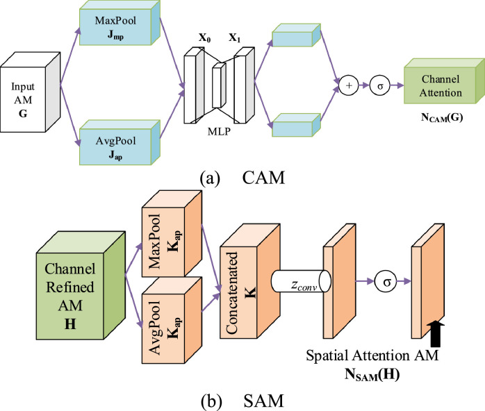
CAM is firstly defined. Both max pooling (MP) $z_{mp}$ and average pooling (AP) $z_{mp}$ are employed, making two features ${\mathbf{J}}_{\mathbf{ap}}$ and ${\mathbf{J}}_{\mathbf{mp}}$ as shown in Fig. 5 (a).

$$\{\begin{array}{c}{\mathbf{J}}_{\mathbf{ap}}=z_{ap}\left(\mathbf{G}\right)\\ {\mathbf{J}}_{\mathbf{mp}}=z_{mp}\left(\mathbf{G}\right)\end{array}$$ (3)

Fig. 5.

Flowchart of two modules.

Both ${\mathbf{J}}_{\mathbf{ap}}$ and ${\mathbf{J}}_{\mathbf{mp}}$ are thenceforth sent to a shared multi-layer perceptron (MLP) to make the output AMs, that are then merged via element-wise summation $\oplus$. The merged sum $z_{mlp}\left[{\mathbf{J}}_{\mathbf{ap}}\right]\oplus z_{mlp}\left[{\mathbf{J}}_{\mathbf{mp}}\right]$ is lastly forwarded to $\sigma$. That is,

$${\mathbf{N}}_{\mathbf{CAM}}\left(\mathbf{G}\right)=\sigma \left\{z_{mlp}\left[{\mathbf{J}}_{\mathbf{ap}}\right]\oplus z_{mlp}\left[{\mathbf{J}}_{\mathbf{mp}}\right]\right\}$$ (4)

where $\sigma$ is sigmoid function.

To decrease the parameter space, the hidden size of MLP is fixed to ${\mathbb{R}}^{C/r\times 1\times 1}$, where $r$ stands for the reduction ratio. Assume ${\mathbf{X}}_0\in {\mathbb{R}}^{C/r\times C}$ and ${\mathbf{X}}_1\in {\mathbb{R}}^{C\times C/r}$ mean the MLP weights (See Fig. 5a), respectively, equation (4) can be rewritten as:

$${\mathbf{N}}_{\mathbf{CAM}}\left(\mathbf{G}\right)=\sigma \left\{{\mathbf{X}}_1\left[{\mathbf{X}}_0\left({\mathbf{J}}_{\mathbf{ap}}\right)\right]\oplus {\mathbf{X}}_1\left[{\mathbf{X}}_0\left({\mathbf{J}}_{\mathbf{mp}}\right)\right]\right\}$$ (5)

Note ${\mathbf{X}}_0$ and ${\mathbf{X}}_1$ are shared by both ${\mathbf{J}}_{\mathbf{ap}}$ and ${\mathbf{J}}_{\mathbf{mp}}$. Fig. 5(a) displays the diagram of CAM.

4.3. Spatial Attention Module

Next, SAM is defined in Fig. 5(b). The spatial attention module ${\mathbf{N}}_{\mathbf{SAM}}$ is a complementary procedure to the previous CAM ${\mathbf{N}}_{\mathbf{CAM}}$. The average pooling $z_{ap}$ and max pooling $z_{mp}$ are harnessed again to the channel-refined activation map $\mathbf{H}$,

$$\{\begin{array}{c}{\mathbf{K}}_{\mathbf{ap}}=z_{ap}\left(\mathbf{H}\right)\\ {\mathbf{K}}_{\mathbf{mp}}=z_{mp}\left(\mathbf{H}\right)\end{array}$$ (6)

Both ${\mathbf{K}}_{\mathbf{ap}}$ and ${\mathbf{K}}_{\mathbf{mp}}$ are two dimensional AMs: ${\mathbf{K}}_{\mathbf{ap}}\in {\mathbb{R}}^{1\times H\times W}\wedge {\mathbf{K}}_{\mathbf{mp}}\in {\mathbb{R}}^{1\times H\times W}$. They are concatenated via concatenation function $z_{con}$ together along the channel dimension as

$$\mathbf{K}=z_{con}\left({\mathbf{K}}_{\mathbf{ap}},{\mathbf{K}}_{\mathbf{mp}}\right)$$ (7)

Afterwards, the concatenated AM is passed into a standard convolution $z_{conv}$ with the size of $7\times 7$, followed by sigmoid function $\sigma$. Overall, we attain:

$${\mathbf{N}}_{\mathbf{SAM}}\left(\mathbf{H}\right)=\sigma \left\{z_{conv}\left[\mathbf{K}\right]\right\}$$ (8)

The ${\mathbf{N}}_{\mathbf{SAM}}\left(\mathbf{H}\right)$ is then element-wisely multiplied by $\mathbf{H}$ to get the final refined AE $\mathbf{I}$. See Equation (2). The diagram of SAM is portrayed in Fig. 5(b).

4.4. Single Input and Multiple Input Deep Convolutional Attention Networks

In this study, we proposed a novel multiple-input deep convolutional attention network (MIDCAN) based on the ideas of CBAM and multiple-input. The structure of this proposed MIDCAN is determined by trial-and-error method. The variable $m$ in each block varies, and we found the best values are chosen in the range from $\left[1,3\right]$. We tested values larger than 3, which increase the computation burden, but the performances do not increase.

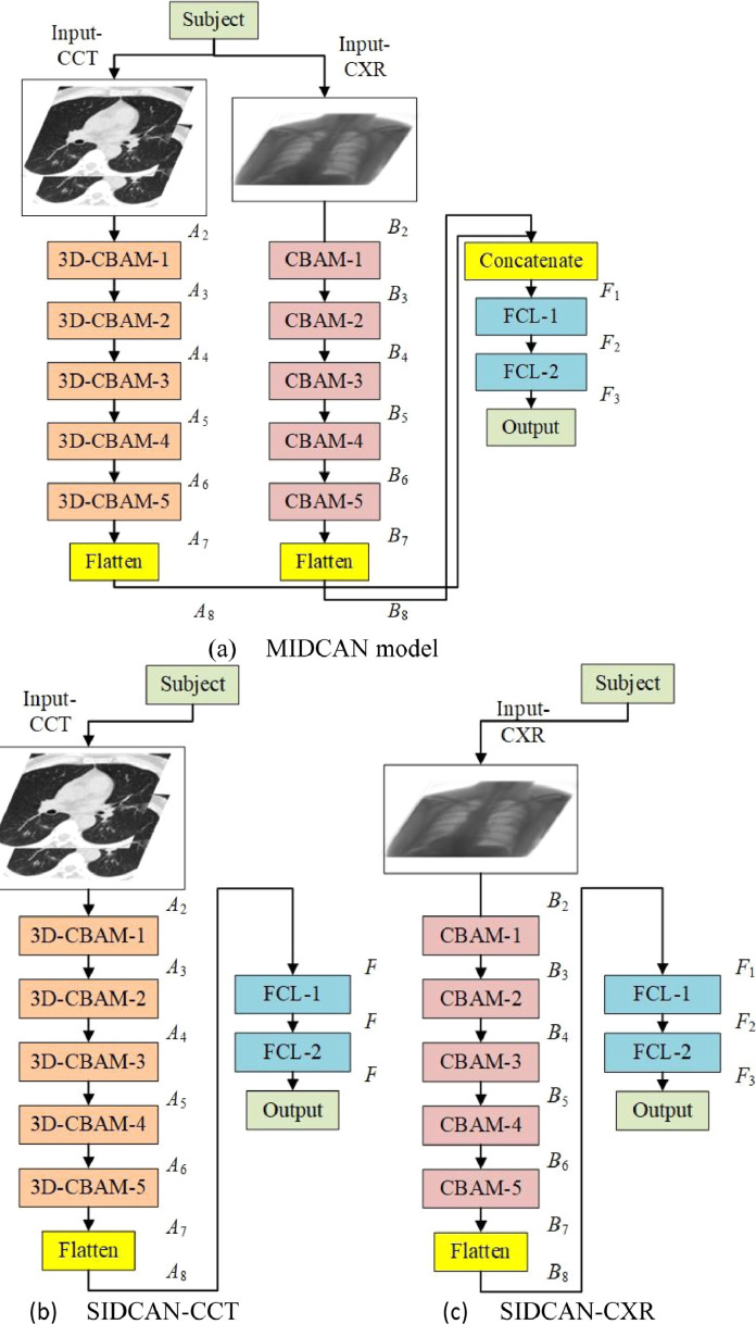
The structure of proposed shown below in Fig. 6 (a), which is composed of two inputs. The left input is “Input-CCT” where CCT images are passed into the network. The right input is “Input-CXR” where CXR images are passed into the network. Suppose $N_C^{CCT}$ and $N_C^{CXR}$ stand for the number of CBAM blocks individually. We set $N_C^{CCT}=N_C^{CXR}=5$ in this study by trial-and-error.

Fig. 6.

Variables and sizes of AMs of three proposed models.

For the left branch, the CCT input $A_2$ goes through $N_C^{CCT}$ 3D-CBAMs and generates the output AM $A_7$, which is then flattened into $A_8$. Similarly, the CXR input at right branch $B_2$ goes through $N_C^{CXR}$ 2D-CBAMs, generates the output AM $B_7$, which is flattened into $B_8$. The deep CCT features and deep CXR features are then concatenated via concatenation function $z_{con}$ as

$$\text{MIDCAN}:F_1=z_{con}\left(A_8,B_8\right)$$ (9)

Here note than in our experiments, we use ablation studies, where we set two models: single-input deep convolutional attention network (SIDCAN) models, which remove the left and right branches, respectively. The first SIDCAN model, shown in Fig. 6(b), will only use CCT features, i.e.,

$$\text{SIDCAN}-\text{CCT}:F_1=A_8$$ (10)

This model is given a short name as SIDCAN-CCT.

The second SIDCAN model will only use CXR features, i.e.,

$$\text{SIDCAN}-\text{CXR}:F_1=B_8$$ (11)

This model is named as SIDCAN-CXR. Its flowchart is displayed in Fig. 6(c). Those two models will used as comparison method in our experiments.

The feature $F_1$ is then passed to two fully-connected layers [22]. The first FCL contains 500 neurons, and the last FCL contains $N_C$ neurons, where $N_C$ stands for the number of classes. In this study $N_C=2$. Finally, a softmax layer [23] turns the $F_3$ to probability. The loss function of this MIDCAN is cross entropy [24] function.

Table 2 gives the details of proposed MIDCAN. For the kernel parameter in Table 2, [3 × 3 × 3, 16]x3, [/2/2/2] stands for 3 repetitions of 16 filters with each size of $3\times 3\times 3$, following by a pooling with pooling factor of 2, 2, and 2 along three dimensions, respectively. In FCL stage, the kernel parameter gives the size of weight matrix and bias vector, respectively.

Table 2.

Details of proposed MIDCAN model.

Name	Kernel Parameter	Variable and size
Input-CCT		$size\left(A_2\right)=256\times 256\times 16$
3D-CBAM-1	[3 × 3 × 3, 16]x3, [/2/2/2]	$size\left(A_3\right)=128\times 128\times 8\times 16$
3D-CBAM-2	[3 × 3 × 3, 32]x2, [/2/2/1]	$size\left(A_4\right)=64\times 64\times 8\times 32$
3D-CBAM-3	[3 × 3 × 3, 32]x2, [/2/2/2]	$size\left(A_5\right)=32\times 32\times 4\times 32$
3D-CBAM-4	[3 × 3 × 3, 64]x2, [/2/2/1]	$size\left(A_6\right)=16\times 16\times 4\times 64$
3D-CBAM-5	[3 × 3 × 3, 64]x2, [/2/2/2]	$size\left(A_7\right)=8\times 8\times 2\times 64$
Flatten		$size\left(A_8\right)=8192$
Input-CXR		$size\left(B_2\right)=256\times 256$
CBAM-1	[3 × 3, 16]x3, [/2/2]	$size\left(B_3\right)=128\times 128\times 16$
CBAM-2	[3 × 3, 32]x2, [/2/2]	$size\left(B_4\right)=64\times 64\times 32$
CBAM-3	[3 × 3, 64]x2, [/2/2]	$size\left(B_5\right)=32\times 32\times 64$
CBAM-4	[3 × 3, 64]x2, [/2/2]	$size\left(B_6\right)=16\times 16\times 64$
CBAM-5	[3 × 3, 128]x2, [/2/2]	$size\left(B_7\right)=8\times 8\times 128$
Flatten		$size\left(B_8\right)=8192$
Concatenate		$size\left(F_1\right)=16,384$
FCL-1	500 × 16384, 500 × 1	$size\left(F_2\right)=500$
FCL-2	2 × 500, 2 × 1	$size\left(F_3\right)=2$
Softmax

4.5. 18-way data augmentation

Data augmentation (DA) [25] is an important utensil over the training set to avoid overfitting of classifiers when applied to test set. Meanwhile, DA can overcome the small-size dataset problem. Recently, Wang (2021) [26] proposed a novel 14-way data augmentation (DA), which used seven different DA techniques to the preprocessed training image $v\left(k\right)$ and its horizontal mirrored image $v^H\left(k\right)$, respectively. Cheng (2021) [27] presented a 16-way DA, and used PatchShuffle technique to avoid overfitting.

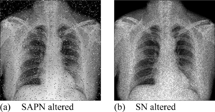
This study enhances the 14-way DA method [26] to 18-way DA, by adding two new DA methods: salt-and-pepper noise (SAPN) and speckle noise (SN) on both $v\left(k\right)$ and $v^H\left(k\right)$. Use $v\left(k\right)$ as an example, the SAPN altered image is symbolized as $v^{SAPN}\left(k\right)$ with its values are set as

$$\{\begin{array}{c}\mathbf{R}\left(v^{SAPN}=v\right)=1-{\gamma }_d^{sa},\hfill \\ \mathbf{R}\left(v^{SAPN}=v_{min}\right)=\frac{{\gamma }_d^{sa}}{2},\hfill \\ \mathbf{R}\left(v^{SAPN}=v_{max}\right)=\frac{{\gamma }_d^{sa}}{2},\hfill \end{array}$$ (12)

where ${\gamma }_d^{sa}$ stands for noise density, and $\mathbf{R}$ the probability function. $v_{\text{min}}$ and $v_{\text{max}}$ correspond to black and white colors, respectively.

On the other side, the SN altered image is defined as

$$v^{SN}\left(k\right)=v\left(k\right)+\mathbb{U}\times v\left(k\right),$$ (13)

where $\mathbb{U}$ is a uniformly distributed random noise, of which the mean and variance are symbolized as $U_m^{sn}$ and $U_v^{sn}$, respectively. Take Fig. 3(b) as the example, Fig. 7 (a-b) display the SAPN and SN altered images, respectively. Due to the page limit, the results of other DA are not shown in this paper.

Fig. 7.

Examples of newly proposed DA methods.

Let $M_a$ stands for the number of DA techniques to the preprocessed image $v\left(k\right)$, and $M_b$ stands for the number of new generated images for each DA. This proposed $\left(2\times M_a\right)$-way DA algorithm is a four-step algorithm depicted below:

First, $M_a$ geometric/photometric/noise-injection DA transforms are utilized on preprocessed train image $v\left(k\right)$,. We use $w_{\left(m\right)}^{DA},m=1,\dots ,M_a$ to denote each DA operation. See each DA operations $w_{\left(m\right)}^{DA}$ yields $M_b$ new images. Thus, for a given image $t\left(k\right)$, we yield $M_a$ different data set $w_{\left(m\right)}^{DA}\left[v\left(k\right)\right],m=1,\cdots ,M_a$, and each dataset contains $M_b$ new images.

Second, horizontally mirrored image is generated as

$$v^H\left(k\right)=z_M\left[v\left(k\right)\right],$$ (14)

where $z_M$ means horizontal mirror function.

Third, all the $M_a$ DA methods are carried out on the mirror image $v^H\left(k\right)$, and generate $M_a$ different dataset $w_{\left(m\right)}^{DA}\left[v^H\left(k\right)\right],m=1,\cdots ,M_a$.

Four, the raw image $v\left(k\right)$, the horizontally mirrored image $v^H\left(k\right)$, all $M_a$-way results of preprocessed image $w_{\left(m\right)}^{DA}\left[v\left(k\right)\right],m=1,\cdots ,M_a$, and $M_a$-way DA results of horizontally mirrored image $w_{\left(m\right)}^{DA}\left[v^H\left(k\right)\right],m=1,\cdots ,M_a$, are fused together using concatenation function $z_{CON}$, as defined in Eq. (9).

The final combined dataset is defined as $\Lambda$

$$v\left(k\right)\mapsto \Lambda =z_{con}\left\{\begin{array}{cc}v\left(k\right)& v^H\left(k\right)\\ \underset{M_b}{\underbrace{w_{\left(1\right)}^{DA}\left[v\left(k\right)\right]}}& \underset{M_b}{\underbrace{w_{\left(1\right)}^{DA}\left[v^H\left(k\right)\right]}}\\ \cdots & \cdots \\ \underset{M_b}{\underbrace{w_{\left(M_a\right)}^{DA}\left[v\left(k\right)\right]}}& \underset{M_b}{\underbrace{w_{\left(M_a\right)}^{DA}\left[v^H\left(k\right)\right]}}\end{array}\right\}$$ (15)

Therefore, one image $v\left(k\right)$ will generate

$$\left|\Lambda \right|=2\times M_a\times M_b+2$$ (16)

images (including the original image $v\left(k\right)$). Note in our dataset, different $M_b$ will be assigned to CCT training images and CXR images since CCT images are 3D and CXR images are 2D. That means for each DA, we have $M_b^{CCT}$ new images for each CCT image and $M_b^{CXR}$ new images for each CXR image.

4.6. Implementation and evaluation

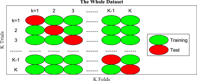
$K$-fold cross validation is employed on both datasets. Suppose confusion matrix $\mathbf{J}$ over r-th ($1\le r\le R$) run and k-th ($1\le k\le K$) fold is defined as

$$\mathbf{J}\left(r,k\right)=\left[\begin{array}{cc}{j}_{11}\left(r,k\right)& j_{12}\left(r,k\right)\\ j_{21}\left(r,k\right)& j_{22}\left(r,k\right)\end{array}\right]$$ (17)

where $\left(j_{11},j_{12},j_{21},j_{22}\right)$ stand for TP, FN, FP, and TN, respectively. P stands for positive class, i.e., COVID-19, and N means negative class, i.e., healthy control. $k$ represents the index of trial/fold, and r stands for the index of run. At $k$-th trial, the $k$-th fold is used as test, and all the left folds are used as training,

Note that $\mathbf{J}\left(r,k\right)$ is calculated based on each test fold, and are then summarized across all $K$ trials, as shown in Fig. 8 . Afterwards, we get the confusion matrix at r-th run $\mathbf{J}\left(r\right)$ as

$$\mathbf{J}\left(r\right)=\sum _{k=1}^K\mathbf{J}\left(r,k\right)$$ (18)

Fig. 8.

Diagram of one run of $K$-fold cross validation.

Seven indicators $\overrightarrow{\tau }\left(r\right)$ are computed based on the confusion matrix over r-th run $\mathbf{J}\left(r\right)$.

$$\mathbf{J}\left(r\right)\mapsto \overrightarrow{\eta }\left(r\right)=\left[{\eta }_1\left(r\right),{\eta }_2\left(r\right),\cdots ,{\eta }_7\left(r\right)\right],$$ (19)

where first four indicators are: ${\eta }_1$ sensitivity, ${\eta }_2$ specificity, ${\eta }_3$ precision, and ${\eta }_4$ accuracy. Those four indicators are commonly used. Their definitions can be found easily. ${\eta }_5$ is F1 score.

$${\eta }_5\left(r\right)=\frac{2\times j_{11}\left(r\right)}{2\times j_{11}\left(r\right)+j_{12}\left(r\right)+j_{21}\left(r\right)}$$ (20)

${\eta }_6$ is Matthews correlation coefficient (MCC)

$${\eta }_6\left(r\right)=\frac{j_{11}\left(r\right)\times j_{22}\left(r\right)-j_{21}\left(r\right)\times j_{12}\left(r\right)}{\sqrt{\left[j_{11}\left(r\right)+j_{21}\left(r\right)\right]\times \left[j_{11}\left(r\right)+j_{12}\left(r\right)\right]\times \left[j_{22}\left(r\right)+j_{21}\left(r\right)\right]\times \left[j_{22}\left(r\right)+j_{12}\left(r\right)\right]}}$$ (21)

and ${\eta }_7$ is the Fowlkes–Mallows index (FMI).

$${\eta }_7\left(r\right)=\sqrt{\frac{j_{11}\left(r\right)}{j_{11}\left(r\right)+l_{21}\left(r\right)}\times \frac{j_{11}\left(r\right)}{j_{11}\left(r\right)+j_{21}\left(r\right)}}$$ (22)

There are two indicators ${\eta }_4$ and ${\eta }_6$ using all the four basic measures $\left(j_{11},j_{12},j_{21},j_{22}\right)$. Considering the range of ${\eta }_4$ is $0\le {\eta }_4\le 1$, and the range of ${\eta }_6$ is $-1\le {\eta }_6\le +1$, we finally choose ${\eta }_6$ as the most important indicator. Besides, Chicco, Totsch (2021) [28] stated that MCC is more reliable than many other indicators.

Above procedure is one run of $K$-fold cross validation. We run the $K$-fold cross validation $R$ runs. The mean and standard deviation (MSD) of all seven indicators ${\eta }_m\left(m=1,\dots ,7\right)$ are calculated over all $R$ runs.

$$\{\begin{array}{c}\mu \left({\eta }_m\right)=\frac{1}{R}\times \sum _{r=1}^R{\eta }_m\left(r\right)\hfill \\ \sigma \left({\eta }_m\right)=\sqrt{\frac{1}{R-1}\times \sum _{r=1}^R{\left|{\eta }_m\left(r\right)-\mu \left({\eta }_m\right)\right|}^2}\hfill \end{array}$$ (23)

where $\mu$ stands for the mean value, and $\sigma$ stands for the standard deviation. The MSDs are reported in the format of $\eta =\mu \left(\eta \right)\pm \sigma \left(\eta \right)$.

5. Experiments, results, and discussions

5.1. Parameter setting

Table 3 itemizes the parameter setting. Here the minimum value and maximum value of our images are set to 0 and 255, respectively. The size of preprocessed CCT images and CXR images are set to $256\times 256\times 16$ and $256\times 256$, respectively. The number of CBAM blocks for CCT and CXR branches are set to 5. The noise density of SAPN is set to 0.05. The mean and variance of uniform distributed noise in SN are set to 0 and 0.05, respectively. Nine different DA methods are used, so we have an 18-way DA if we consider both raw training image and its horizontal mirrored image. For each DA, 30 new images are generated for each CXR image, and 90 new images are generated for each CCT image. The number of $K$-fold is set to $K=10$. We run our model $R=10$ runs.

Table 3.

Parameter setting.

Parameter	Value
$\left(v_{min},v_{,max}\right)$	(0, 255)
$H^{CCT}\times W^{CCT}\times C^{CCT}$	$256\times 256\times 16$
$H^{CXR}\times W^{CXR}$	$256\times 256$
$N_C^{CCT}$	5
$N_C^{CXR}$	5
${\gamma }_d^{sa}$	0.05
$U_m^{sn}$	0
$U_v^{sn}$	0.05
$M_a$	9
$M_b^{CXR}$	30
$M_b^{CCT}$	90
$K$	10
$R$	10

5.2. Statistics of proposed MIDCAN

We use two modalities, CCT and CXR, in this experiment. The structure of our model is shown in Fig. 6(a). The statistical results of proposed MIDCAN are shown in Table 4 . As it shows, the sensitivity, specificity, precision and accuracy are 98.10±1.88, 97.95±2.26, 97.92±2.24, and 98.02±1.35, respectively. Moreover, the F1 score is 97.98±1.37, the MCC is 96.09±2.66, and FMI is 97.99±1.36.

Table 4.

Statistical results of proposed MIDCAN model.

Run	${\eta }_1$	${\eta }_2$	${\eta }_3$	${\eta }_4$	${\eta }_5$	${\eta }_6$	${\eta }_7$
1	97.62	100.00	100.00	98.84	98.80	97.70	98.80
2	97.62	97.73	97.62	97.67	97.62	95.35	97.62
3	100.00	100.00	100.00	100.00	100.00	100.00	100.00
4	100.00	97.73	97.67	98.84	98.82	97.70	98.83
5	95.24	97.73	97.56	96.51	96.39	93.04	96.39
6	100.00	93.18	93.33	96.51	96.55	93.26	96.61
7	100.00	100.00	100.00	100.00	100.00	100.00	100.00
8	97.62	95.45	95.35	96.51	96.47	93.05	96.48
9	95.24	100.00	100.00	97.67	97.56	95.44	97.59
10	97.62	97.73	97.62	97.67	97.62	95.35	97.62
MSD	98.10 ±1.88	97.95 ±2.26	97.92 ±2.24	98.02 ±1.35	97.98 ±1.37	96.09 ±2.66	97.99 ±1.36

5.3. Effect of multimodality and attention mechanism

We compare multiple-modality against single-modality. Two models, viz., SIDCAN-CCT and SIDCAN-CXR, shown in Fig. 6(b-c) are used. Meanwhile, using attention and not using attention are compared.

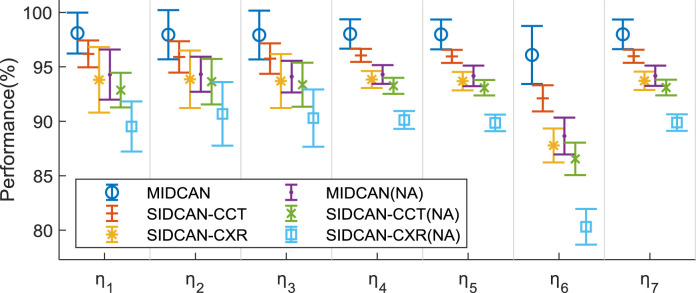
The comparison results are shown in Table 5 , where NA means no attention. Fig. 9 presents the error bar comparison of all the six setting. Comparing using attention against without using attention, we can observe the attention mechanism does help improve the classification performance, which is coherent with the conclusion of Ref. [21].

Table 5.

Comparison of different settings.

Method	${\eta }_1$	${\eta }_2$	${\eta }_3$	${\eta }_4$	${\eta }_5$	${\eta }_6$	${\eta }_7$
MIDCAN	98.10 ±1.88	97.95 ±2.26	97.92 ±2.24	98.02 ±1.35	97.98 ±1.37	96.09 ±2.66	97.99 ±1.36
SIDCAN -CCT	96.19 ±1.23	95.91 ±1.44	95.76 ±1.40	96.05 ±0.60	95.96 ±0.60	92.11 ±1.20	95.97 ±0.60
SIDCAN-CXR	93.81 ±3.01	93.86 ±2.64	93.70 ±2.48	93.84 ±0.78	93.69 ±0.85	87.78 ±1.56	93.72 ±0.84
MIDCAN (NA)	94.29 ±2.30	94.32 ±1.61	94.10 ±1.45	94.30 ±0.86	94.17 ±0.94	88.65 ±1.69	94.18 ±0.93
SIDCAN-CCT(NA)	92.86 ±1.59	93.64 ±2.09	93.36 ±2.02	93.26 ±0.74	93.08 ±0.71	86.55 ±1.49	93.10 ±0.72
SIDCAN-CXR(NA)	89.52 ±2.30	90.68 ±2.92	90.29 ±2.63	90.12 ±0.82	89.85 ±0.76	80.31 ±1.64	89.88 ±0.76

Fig. 9.

Error bar comparison of six different settings.

Meanwhile, if we compare MIDCAN with two SIDCAN models, we can conclude that multimodality has the better performance than single modalities (both CT and CXR).

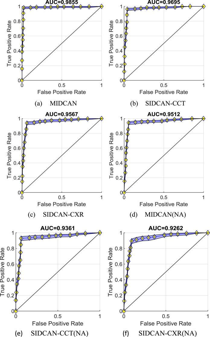
Fig. 10 displays the ROC curves of six settings. The blue patch corresponds to the lower bound and upper bound. For the first three models using attention, we can observe their AUCs are 0.9855, 0.9695, and 0.9567 for MIDCAN, SIDCAN-CCT, and SIDCAN-CXR, respectively. If removing the CBAM module, we can observe from the bottom part of Fig. 10, that the corresponding AUCs decrease to 0.9512, 0.9361, and 0.9262, respectively. In addition, multimodality is proven to give better performance than using single-modality.

Fig. 10.

ROC curves of six settings.

5.4. Explainability of proposed model

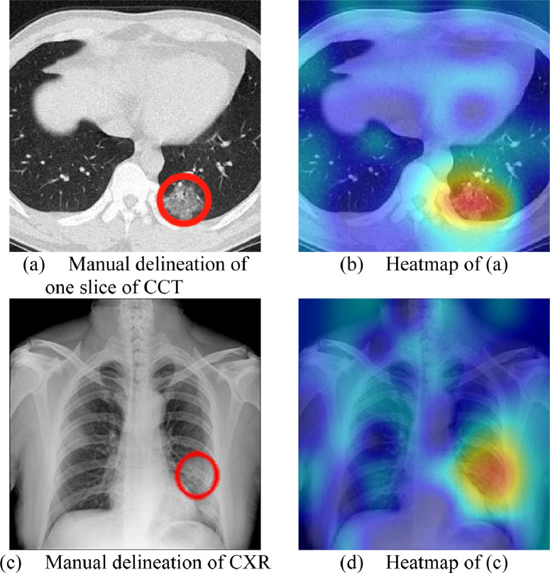
Fig. 11 presents the manual delineation and heatmap results of Fig. 3. The heatmap images are generated via Grad-CAM method [29].

Fig. 11.

Manual delineation and heatmap results of one patient.

From Fig. 11, we can observe the proposed MIDCAN model is able to capture the lesions of both CCT image and CXR image accurately. This explainability via Grad-CAM can help the doctors, radiologists, and patients to better understand how our AI model works.

5.5. Comparison to State-of-the-art approaches

We compare the proposed method “MIDCAN” with 8 state-of-the-art methods: GLCM [7], WE-BBO [8], WRE [9], FSVC [10], OTLS [11], MRA [13], GG [14], SMO [15]. Those methods were carried out on single modality dataset depending on their original paper reported (either CCT or CXR), so we test those methods in the corresponding SIDCAN models and single-modality dataset.

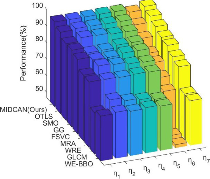
All the methods were evaluated via 10 runs of 10-fold cross validation. The MSD results $\overrightarrow{\eta }$ of all approaches on ten runs of 10-fold cross validation are pictured in Fig. 12 , which sorts all the methods in terms of ${\eta }_6$, and itemized in Table 6 .

Fig. 12.

3D bar plot of approach comparison.

Table 6.

Comparison with SOTA approaches (Unit: %).

Approach	${\eta }_1$	${\eta }_2$	${\eta }_3$	${\eta }_4$	${\eta }_5$	${\eta }_6$	${\eta }_7$
GLCM [7]	71.90 ±4.02	78.18 ±3.89	76.04 ±2.41	75.12 ±0.98	73.80 ±1.49	50.35 ±1.91	73.89 ±1.39
WE-BBO [8]	74.05 ±4.82	74.77 ±3.93	73.83 ±1.84	74.42 ±0.78	73.81 ±1.65	48.98 ±1.65	73.88 ±1.67
WRE [9]	86.43 ±3.18	86.36 ±3.86	86.01 ±3.13	86.40 ±0.56	86.12 ±0.39	72.95 ±1.15	86.17 ±0.40
FSVC [10]	91.90 ±2.56	90.00 ±2.44	89.85 ±1.99	90.93 ±0.49	90.82 ±0.55	81.97 ±0.99	90.85 ±0.56
OTLS [11]	95.95 ±2.26	96.59 ±1.61	96.45 ±1.56	96.28 ±1.07	96.17 ±1.13	92.60 ±2.09	96.19 ±1.12
MRA [13]	86.43 ±3.90	90.45 ±2.79	89.71 ±2.63	88.49 ±2.08	87.98 ±2.27	77.09 ±4.17	88.02 ±2.26
GG [14]	93.33 ±2.70	90.00 ±4.44	90.13 ±3.81	91.63 ±1.53	91.61 ±1.35	83.49 ±2.84	91.67 ±1.30
SMO [15]	93.10 ±2.37	95.23 ±2.50	94.99 ±2.45	94.19 ±1.10	93.99 ±1.13	88.45 ±2.16	94.02 ±1.11
MIDCAN (Ours)	98.10 ±1.88	97.95 ±2.26	97.92 ±2.24	98.02 ±1.35	97.98 ±1.37	96.09 ±2.66	97.99 ±1.36

From Table 6, we can observe that this proposed MIDCAN outperforms all the other 8 comparison baseline methods in terms of all indicators.

The reason why our MIDCAN method is the best lie in following three facts: (i) we propose to use multiple modality instead of traditional single modality; (ii) CBAM is used in our network that attention mechanism can help our AI model focuses on the lesion region; (iii) multiple-way data augmentation is employed to overcome overfitting.

6. Conclusion

This paper proposed a novel multiple input deep convolutional attention network (MIDCAN) model for diagnosis of COVID-19. The results show our method achieves a sensitivity of 98.10±1.88%, a specificity of 97.95±2.26%, and an accuracy of 98.02±1.35%.

In the future researches, we shall carry out several attempts: (i) expand our dataset; (ii) include other advanced network strategies, such as graph neural network; (iii) collect IoT signals of subjects.

Declaration of Competing Interest

The authors declare that they have no known competing financial interests or personal relationships that could have appeared to influence the work reported in this paper.

Edited by: Maria De Marsico

References

- 1.Turgutalp K., et al. Determinants of mortality in a large group of hemodialysis patients hospitalized for COVID-19. BMC Nephrol. 2021;22(1):10. doi: 10.1186/s12882-021-02233-0. Article ID. 29. [DOI] [PMC free article] [PubMed] [Google Scholar]
- 2.Hall A.J. The United Kingdom joint committee on vaccination and immunisation. Vaccine. 2010;28:A54–A57. doi: 10.1016/j.vaccine.2010.02.034. [DOI] [PubMed] [Google Scholar]
- 3.Sakanashi D., et al. Comparative evaluation of nasopharyngeal swab and saliva specimens for the molecular detection of SARS-CoV-2 RNA in Japanese patients with COVID-19. J. Infect. Chemother. 2021;27(1):126–129. doi: 10.1016/j.jiac.2020.09.027. [DOI] [PMC free article] [PubMed] [Google Scholar]
- 4.Giannitto C., et al. Chest CT in patients with a moderate or high pretest probability of COVID-19 and negative swab. Radiol. Med. (Torino) 2020;125(12):1260–1270. doi: 10.1007/s11547-020-01269-w. [DOI] [PMC free article] [PubMed] [Google Scholar]
- 5.Draelos R.L., et al. Machine-learning-based multiple abnormality prediction with large-scale chest computed tomography volumes. Med. Image Anal. 2021;67:12. doi: 10.1016/j.media.2020.101857. Article ID. 101857. [DOI] [PMC free article] [PubMed] [Google Scholar]
- 6.Braga A., et al. When less is more: regarding the use of chest X-ray instead of computed tomography in screening for pulmonary metastasis in postmolar gestational trophoblastic neoplasia. Br. J. Cancer. 2021 doi: 10.1038/s41416-020-01209-5. [DOI] [PMC free article] [PubMed] [Google Scholar]
- 7.Chen Y. in COVID-19: Prediction, Decision-Making, and its Impacts. Springer Singapore; Singapore: 2020. Covid-19 classification based on gray-level co-occurrence matrix and support vector machine; pp. 47–55. K.C. Santosh and A. Joshi, Editors. [Google Scholar]
- 8.Yao X. in COVID-19: Prediction, Decision-Making, and its Impacts. Springer; 2020. COVID-19 detection via wavelet entropy and biogeography-based optimization; pp. 69–76. K.C. Santosh and A. Joshi, Editors. [Google Scholar]
- 9.Wu X. Diagnosis of COVID-19 by wavelet Renyi entropy and three-segment biogeography-based optimization. Int. J. Comput. Intell. Syst. 2020;13(1):1332–1344. [Google Scholar]
- 10.El-kenawy E.S.M., et al. Novel feature selection and voting classifier algorithms for COVID-19 classification in CT images. IEEE Access. 2020;8:179317–179335. doi: 10.1109/ACCESS.2020.3028012. [DOI] [PMC free article] [PubMed] [Google Scholar]
- 11.Satapathy S.C. Covid-19 diagnosis via DenseNet and optimization of transfer learning setting. Cognitive Comput. 2021 doi: 10.1007/s12559-020-09776-8. [DOI] [PMC free article] [PubMed] [Google Scholar]
- 12.Saood A., et al. COVID-19 lung CT image segmentation using deep learning methods: U-Net versus SegNet. BMC Med. Imaging. 2021;21(1):10. doi: 10.1186/s12880-020-00529-5. Article ID. 19. [DOI] [PMC free article] [PubMed] [Google Scholar]
- 13.Ismael A.M., et al. The investigation of multiresolution approaches for chest X-ray image based COVID-19 detection. Health Inf. Sci. Syst. 2020;8(1) doi: 10.1007/s13755-020-00116-6. Article ID. 29. [DOI] [PMC free article] [PubMed] [Google Scholar]
- 14.Loey M., et al. Within the lack of chest COVID-19 X-ray dataset: a novel detection model based on GAN and deep transfer learning. Symmetry-Basel. 2020;12(4) Article ID. 651. [Google Scholar]
- 15.Togacar M., et al. COVID-19 detection using deep learning models to exploit Social Mimic Optimization and structured chest X-ray images using fuzzy color and stacking approaches. Comput. Biol. Med. 2020;121:12. doi: 10.1016/j.compbiomed.2020.103805. Article ID. 103805. [DOI] [PMC free article] [PubMed] [Google Scholar]
- 16.Das A.K., et al. Automatic COVID-19 detection from X-ray images using ensemble learning with convolutional neural network. Pattern Anal. Appl. 2021:14. doi: 10.1007/s10044-021-00970-4. [DOI] [Google Scholar]
- 17.Susukida R., et al. Data management in substance use disorder treatment research: Implications from data harmonization of National Institute on Drug Abuse-funded randomized controlled trials. Clin. Trials. 2021:11. doi: 10.1177/1740774520972687. [DOI] [PubMed] [Google Scholar]
- 18.Kumari K., et al. Multi-modal aggression identification using convolutional neural network and binary particle swarm optimization. Future Generat. Comput. Syst. Int. J. Escience. 2021;118:187–197. [Google Scholar]
- 19.Hamer A.M., et al. Replacing human interpretation of agricultural land in Afghanistan with a deep convolutional neural network. Int. J. Remote Sens. 2021;42(8):3017–3038. [Google Scholar]
- 20.Hu J., et al. Squeeze-and-excitation networks. IEEE Trans. Pattern Anal. Mach. Intell. 2020;42(8):2011–2023. doi: 10.1109/TPAMI.2019.2913372. [DOI] [PubMed] [Google Scholar]
- 21.Woo S., et al. CBAM: Convolutional block attention module. Proceedings of the European conference on computer vision (ECCV); Munich, Germany; Springer; 2018. pp. 3–19. [Google Scholar]
- 22.Sindi H., et al. Random fully connected layered 1D CNN for solving the Z-bus loss allocation problem. Measurement. 2021;171:8. Article ID. 108794. [Google Scholar]
- 23.Kumar A., et al. Topic-document inference with the gumbel-softmax distribution. IEEE Access. 2021;9:1313–1320. [Google Scholar]
- 24.Sathya P.D., et al. Color image segmentation using Kapur, Otsu and minimum cross entropy functions based on exchange market algorithm. Expert Syst. Appl. 2021;172:30. Article ID. 114636. [Google Scholar]
- 25.Kim S., et al. Synthesis of brain tumor multicontrast MR images for improved data augmentation. Med. Phys. 2021:14. doi: 10.1002/mp.14701. [DOI] [PubMed] [Google Scholar]
- 26.Wang S.-H. Covid-19 classification by FGCNet with deep feature fusion from graph convolutional network and convolutional neural network. Inf. Fusion. 2021;67:208–229. doi: 10.1016/j.inffus.2020.10.004. [DOI] [PMC free article] [PubMed] [Google Scholar]
- 27.Cheng X. PSSPNN: PatchShuffle stochastic pooling neural network for an explainable diagnosis of COVID-19 with multiple-way data augmentation. Comput. Math. Methods Med. 2021;2021 doi: 10.1155/2021/6633755. Article ID. 6633755. [DOI] [PMC free article] [PubMed] [Google Scholar] [Retracted]
- 28.Chicco D., et al. The Matthews correlation coefficient (MCC) is more reliable than balanced accuracy, bookmaker informedness, and markedness in two-class confusion matrix evaluation. Biodata Mining. 2021;14(1):22. doi: 10.1186/s13040-021-00244-z. Article ID. 13. [DOI] [PMC free article] [PubMed] [Google Scholar]
- 29.Selvaraju R.R., et al. Grad-CAM: visual explanations from deep networks via gradient-based localization. Int. J. Comput. Vision. 2020;128(2):336–359. [Google Scholar]