

Abstract
The Autoregressive Latent Trajectory (ALT) model synthesizes the autoregressive model and the latent growth curve model. The ALT model is flexible enough to produce a variety of discrepant model-implied change trajectories. While some researchers consider this a virtue, others have cautioned that this may confound interpretations of the model’s parameters. In this article, we show that some – but not all – of these interpretational difficulties may be clarified mathematically and tested explicitly via likelihood ratio tests (LRTs) imposed on the initial conditions of the model. We show analytically the nested relations among three variants of the ALT model, and the constraints needed to establish equivalences. A Monte Carlo simulation study indicated that LRTs, particularly when used in combination with information criterion measures, can allow researchers to test targeted hypotheses about the functional forms of the change process under study. We further demonstrate when and how such tests may justifiably be used to facilitate our understanding of the underlying process of change using a subsample (N=3995) of longitudinal family income data from the National Longitudinal Survey of Youth.
Keywords: Autoregressive latent trajectory model, Initial condition, Latent growth curve models
More than two decades since the introduction and popularization of the latent growth curve (LGC) models in the social and behavioral sciences (Bryk & Raudenbush, 1987; McArdle & Epstein, 1987; Meredith & Tisak, 1984, 1990; Rogosa & Willett, 1985), LGC models and their extensions have become ever more popular as a tool for studying change. One such extensions is the Autoregressive Latent Trajectory model (ALT; Bollen & Curran, 1999, 2004; Curran & Bollen, 1999, 2001), proposed as a way to synthesize autoregressive (AR) features (Box, Jenkins, Reinsel, & Ljung, 2016; Hamilton, 1994) — or time dependencies between adjacent measurement occasions — into the LGC model. Thus, the ALT model retains the strengths of the LGC model as a way to represent systematic growth/decline patterns and interindividual differences therein, as well as AR features in which the current measurement occasion is allowed to depend on one or more previous occasions.
Despite the strengths of the ALT model as a unification of the AR model and the LGC model, several researchers have brought up cautionary notes concerning the use of the ALT model, as well as potential confusions that may arise from an inferential standpoint (Curran, Howard, Bainter, Lane, & McGinley, 2014; Hamaker, 2005). One cautionary note from Voelkle (2008) is that if the ALT model with a linear latent trajectory is fitted to processes that show nonlinear changes, the AR parameter is often observed to “correct for” this misspecification through inflation in its (absolute) magnitude. Jongerling and Hamaker (2011) also brought up a related note that the ALT model has the flexibility to yield a variety of change trajectories whose functional forms may not be easily deduced from mere inspection of the parameter estimates, which leads to confusions in the interpretations of the parameters. This flexibility is not unanticipated, however, given that AR models have often been used as an approximation model for various change processes (e.g., AR models with time-varying parameters; Prado, West, & Krystal, 2001; Rovine & Molenaar, 2005; Tarvainen, Hiltunen, Ranta-aho, & Karjalainen, 2004). In addition, the AR model also includes as a special case the random walk model — another popular model for approximating many change processes in economics and other sciences (Iacus, 2008; Révész, 1990). Thus, the flexibility of the ALT model in itself does not constitute a problem if it is indeed used as an approximation of change. Greater problems arise, however, when researchers are drawing substantive conclusions — including inferences concerning the nature and sources of the interindividual difference in change — without a clear understanding of the change trajectories implied by the ALT model.
In the present article, we show that some of the assumptions and implications of the ALT model can be clarified via a formal investigation of the initial condition specification (ICS) of the ALT model: that is, the hypothesized structure of the ALT process before and up to the first available observation. While the issue of ICS is typically regarded as a trivial methodological detail in most empirical applications of the ALT model, ICS is a central issue in many longitudinal models that assume lagged dependencies among successive occasions. This issue has been investigated in the context of state-space models (De Jong, 1991; Harvey, 2001), as well as time series models within the structural equation modeling framework (du Toit & Browne, 2007). Misspecification of the distribution and structure of the initial conditions can lead to biased estimation, the consequences of which are especially severe in longitudinal panel data (Chow, Ho, Hamaker, & Dolan, 2010; De Jong, 1991; du Toit & Browne, 2007; Losardo, 2012; Oud, van den Bercken, & Essers, 1990). Importantly, we show analytically that the ALT models with different ICSs can be nested, and likelihood ratio tests (LRTs) may be used in conjunction with other fit indices (e.g., information criterion measures) to perform targeted tests of the assumptions implicated in the ALT model. A Monte Carlo simulation study and an empirical example are provided to demonstrate how different choices of ICS can affect interpretations of modeling results and how LRTs and other fit indices can be used to compare three different variants of the ALT model.
In the sections that follow, we first introduce the ALT modeling framework and the variants of the ALT model considered in the present article. We then analytically show the nested relations among the ALT models with different ICSs, and elucidate the interpretation of the parameters in different models. This is followed by a Monte Carlo simulation study conducted to examine the performance of the LRTs, particularly when used in combination with information criterion measures, in identifying the true ALT model and the consequences of ICS misspecification under different sample-size conditions. We then demonstrate how such tests may be used in analyzing a set of empirical data. We end with a discussion of the key insights from this paper as well as future directions.
The ALT Model
At its core, the ALT model combines the LGC model and the AR model of order 1 within a structural equation modeling framework, yielding:
| (1) |
where t = 2, 3, · · · , T indexes time and i = 1, · · · , N indexes subjects. The ALT model as it stands does not make explicit distributional (e.g., normality) assumptions about the residual errors, ϵit; in addition, there are established estimators that are robust to, or can correct for non-normality. To ease presentation, however, we focus here on the special case in which the residual errors are assumed to be normally distributed with mean zero and variance to facilitate the presentation of our analytic comparisons, which focus on comparisons of the means and covariance structures of different ALT variants. The AR part of the model permits individual i’s y value at time t − 1 to influence the individual’s current y value with AR parameter ρt,t−1. This parameter is held invariant across individuals, but may be freed to vary over time. The person-specific terms, αi and βi, are components of the growth curve portion of the ALT model. These growth curve components are further expressed as equations of
| (2) |
where μα and μβ are the mean of αi and βi across all subjects, ζα,i and ζβ,i the correlated disturbances with zero means, variances of and respectively, and covariance of σα,β. When the AR parameters are not zero, these growth curve components have distinct conceptual meanings, as will be explained later.
As an AR structure is assumed in the ALT model, the process has to be “started up” (Bollen & Curran, 2004; Curran & Bollen, 2001; Hamaker, 2005; Jongerling & Hamaker, 2011). In Figure 1, path diagrams of three variants of the ALT model that only differ in their ICSs are shown, referred to herein as the Predetermined, Ongoing Endogenous, and History-Independent Endogenous ALT models, respectively. These models are all special cases of the ALT model presented thus far, except that they are based on different assumptions about the nature of the process at or prior to the first available time point, which constitute different ICSs of the ALT model. We consider these three variants of ALT model to illustrate the intricate analytical relations between the initial conditions of the ALT model and the resultant model-implied change trajectories. We are assuming in this article that t is coded as 1 at the first available time point and the loading for βi on yit is t − 1, at least for t ≥ 2. The ICSs characterize the distributional characteristics of the process at t = 1. For t = 2, 3, · · · , T, Equations 1–2 apply.
Figure 1.
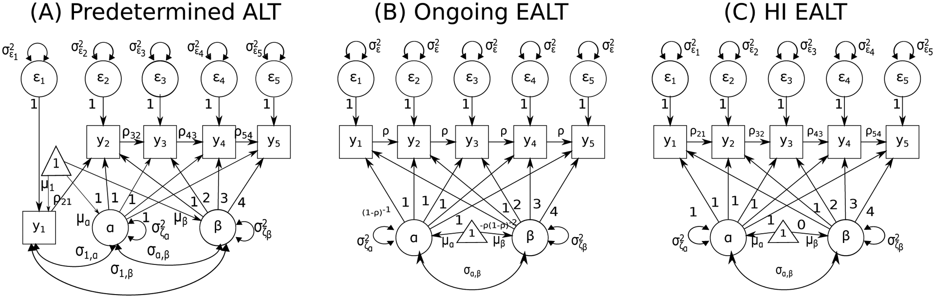
Autoregressive Latent Trajectory (ALT) models with different initial condition specifications. (A), (B), and (C) respectively illustrate the Predetermined, Ongoing Endogenous, and History-Independent Endogenous ALT models.
Predetermined ALT Model
One way of specifying the initial conditions of the ALT process is to treat yi1 as predetermined (Bollen & Curran, 1999, 2004), yielding:
| (3) |
where μ1 represents an unconditional mean of the first time point across all subjects and ϵi1, with mean zero and variance of , stands for an individual’s deviation from μ1 at this time point. The first available observed measurement, yi1, is allowed to covary with αi and βi, with their covariances denoted, respectively as, σ1,α and σ1,β. A path diagram representation of the Predetermined ALT model is shown in Figure 1(A).
With three or fewer measurement occasions, the Predetermined ALT model is not identified. An alternative strategy suggested by Curran and Bollen (2001; see also Bollen and Curran, 2004) is to treat the initial condition for yi1 as endogenous – namely, to explain yi1 as a function of αi and βi. The next two models are examples of such endogenous ALT (EALT) models, and as we will show later, are both nested within the Predetermined ALT model.
Ongoing EALT Model
One EALT model discussed by Curran and Bollen (2001; see also Bollen and Curran, 2004) and elaborated further by Hamaker (2005) assumes that the ALT process has started a long time ago (i.e., as time extends back to negative infinity1) and that ρt,t−1 = ρ, |ρ| < 1, and for all time points. That is, the AR part of the ALT process is assumed to be an ongoing stationary process. In this case, yi1 reduces to (for full derivation details see Bollen and Curran (2004, p. 363–364) and Hamaker (2005, p. 408)):
| (4) |
where ϵi1 has a mean of 0 and variance of . We refer to this model as the Ongoing EALT model to highlight the ongoing stationarity property of the AR portion of the model (see Figure 1(B) for a path diagram representation).
Hamaker (2005) showed that under such ongoing stationarity assumptions, the Ongoing EALT model is algebraically equivalent (i.e., indistinguishable in terms of mean and covariance structures, as well as model fit) to a linear LGC model with AR disturbances, expressed as:
| (5) |
where t = 2, 3, · · · , T, and ϵi,t is assumed to be normally distributed with mean zero and variance . For t = 1, Zi1 comes from a normal distribution with a mean of 0 and variance of . The intercept and slope of individual i in this LGC model with AR disturbances, denoted by Ai and Bi, are related to αi, βi, and ρ from the Ongoing EALT model as (Hamaker, 2005):
| (6) |
hence βi may be interpreted as a scaled or transformed slope factor; however, αi – given that it is a function of both the intercept factor, Ai and the slope factor, Bi – cannot be interpreted directly as the intercept factor. We refer to αi for now as the slope-dependent intercept factor and will clarify its meanings further in the context of other ALT model variants where appropriate. In all subsequent implementations of the Ongoing EALT model, we explicitly incorporate these mapping functions into the Ongoing EALT model to allow the intercept and slope (Ai and Bi) from the LGC model with AR disturbances to be defined within the Ongoing EALT model, while simultaneously estimating αi and βi.
History-Independent EALT Model
The Predetermined and particularly the Ongoing Endogenous ALT models are typically presented in ways that emphasize the need to “start up” the recursions in the ALT process prior to the availability of the first time point. However, in empirical applications, there are many instances in which researchers are only interested in modeling the “local changes” in the process of interest, and regard the potential cumulative effects of earlier time points as negligible or a distinct process that may be omitted from the model (Petersen et al., 2013; Wilson et al., 2013). For instance, Wilson et al. (2013) modeled the cognitive decline of older adults since the onset of dementia as an ALT process. Thus, the intercept marks the onset of the cognitive decline, while the history of cognitive changes prior to the onset of dementia is not of interest to the researchers.
The notion of such a history-independent ALT process is a direct generalization of the LGC model, retaining the expression of yi1 (by substuting t by 1 and setting ρ1,0 = 0 in Equation 1) as:
| (7) |
where the intercept, αi, has the same conceptual meaning as the intercept term in an LGC model (see Figure 1(C) for the path diagram). This alternative ICS is a special case of the endogenous approach to initializing the ALT model; the resultant ALT model, denoted as the History-Independent (HI) EALT model, does not explicitly assume stationarity and time invariance of the ALT process as are posited in the Ongoing EALT model.
Analytic Analysis of the ICSs
In this section, we will show that the Ongoing EALT and the HI EALT models are nested within the Predetermined ALT model, and the constraints needed to specify such nested relations have implications beyond just the first available time point. Specifically, due to the various parameterizations in the ALT models, αi and βi do not always have the same conceptual meanings across the different ALT models. Further difficulties arise in interpreting modeling results when covariates are used to predict interindividual differences in αi and βi. To illustrate these points, we first outline the conditions under which the Predetermined ALT model can be equivalent to the other two EALT models, defined as showing identical model-implied mean and covariance structures, and then discuss the substantive meanings of αi and βi in the context of the three ALT models. Finally, we extend the analytic comparisons to situations involving conditional ALT models, namely, ALT models in which predictors are used to predict the growth-curve related components.
To see that the Ongoing EALT and HI EALT models are nested within the Predetermined ALT model, consider the person-specific vector ηi = [yi1, αi, βi]T, which is assumed to follow a multivariate normal distribution as:
| (8) |
where and are the mean vector and the covariance matrix of the distribution respectively. We refer to μη and Ση as the “initial condition” mean vector and covariance matrix because they contain information that characterizes group and individual differences in initial condition, although we emphasize that elements corresponding to αi and βi, as we will discuss later, may continue to affect the change trajectories beyond the first time point.
The conditions of equivalence for the three variants of the ALT model are summarized in Table 1 (see Appendix A for derivation details). In the Predetermined ALT model, all of the elements in μη and Ση are freely estimated. Adding constraints B1–B5 to the Predetermined ALT model yields the Ongoing EALT model; imposing constraints C1–C5 on the Predetermine ALT model gives rise to the HI EALT model. Thus, by imposing appropriate constraints on the most general Predetermined ALT model, LRTs can be used to evaluate whether it is plausible to relax assumptions of stationarity (Constraint B1 in the Ongoing EALT model), as well as specific postulates concerning the mean (Constraint 2) and variance-covariance structures (Constraints 3–5) of the first observed time point.
Table 1.
Conditions for Equivalence for Autoregressive Latent Trajectory (ALT) models with Different Initial Condition Specifications (ICS)
| ICS | (A) Predetermined | (B) Ongoing EALT | (C) HI EALT |
|---|---|---|---|
| Constraint 1: Stationarity | ρt,t−1 = ρ,∀t, |ρ| < 1, , ∀t | ||
| Constraint 2 | μ1 freely estimated | μ1 = μα | |
| Constraint 3 | freely estimated | ||
| Constraint 4 | σ1,α freely estimated | ||
| Constraint 5 | σ1,β freely estimated | σ1,β = σα,β | |
| Constraint 6: Conditional ALT Models | γα,k, γβ,k, γy,k, k = 1, 2, ⋯ , K freely estimated | , k = 1, 2, ⋯ , K | γy,k = γα,k, k = 1, 2, ⋯ , K |
| Notes | The most general ICS | Nested within (A); (A) & (B) are equivalent with constraints B1–B5 (in unconditional models) or B1–B6 (in conditional models) | Nested within (A); (A) & (C) are equivalent with constraints C2–C5 (in unconditional models) or C1–C6 (in conditional models) |
EALT stands for endogenous ALT models; HI means History-Independent.
Here, we focus on elucidating the roles of αi and βi in the ALT models by evaluating the expected (group average) change trajectory resulted from each ALT variation. Based on Equations 1–2, letting ρt,t−1 = ρ for all t, the group mean trajectory of yit, denoted as μt, can be obtained for all t ≥ 2 as
| (9) |
in the form of a one-step-ahead difference equation and may be solved to yield an expression for μt as a function of time, as opposed to μt−1 (see Appendix B for details). This enables researchers to understand the effects of parameters such as μα and μβ on μt over a range of time points. The solutions for the different ALT models can be shown to be, respectively:
where t ≥ 2, and ρ0 = 1 for any real ρ.
The solution for the Ongoing EALT model (see Equation 10a) suggests that the expected value of yit at time 1 is given by , and the expected change with every unit of increase in time is obtained as . An example of a mean trajectory generated with μα = 1, μβ = 2 and ρ =0.5 is shown in Figure 2(A). This solution form is obtained by imposing stationarity and time invariance assumptions on the ALT process prior to the first available time point (i.e., constraint B1 in Table 1; see also Hamaker, 2005). One important implication is that the mean trajectory implied by the Ongoing EALT model is linear, with an intercept at time 1 of and a slope of (see Equation 10a); by extension, as long as ρ is constrained to be invariant over time, the individual-specific growth/decline trajectories additionally governed by αi and βi are also linear.2 Thus, as shown previously by Hamaker (2005), αi and βi from the Ongoing EALT model can be transformed into the intercept, Ai, and slope, Bi, in an equivalent LGC model with AR disturbances (see the reverse transformation of Equation 6). We refer to βi as the transformed slope factor, and αi as the slope-dependent intercept factor because it is a function of both Ai and Bi.
Figure 2.

(A): Simulated mean trajectory for the unconditional Ongoing Endogenous Autoregressive Latent Trajectory (EALT) model. (B) and (C): Simulated mean trajectories for the unconditional Predetermined Autoregressive Latent Trajectory (ALT) and History-Independent (HI) EALT models (when μα = μ1).
We emphasize here that the statistical equivalence of the Ongoing EALT model and the LGC model with AR disturbances only holds under strict assumptions (i.e., ρ is time-invariant with |ρ| < 1). Even if these assumptions do hold, we acknowledge that statistical equivalence does not imply strict or substantive equivalence, and there are certainly other subtle conceptual differences between the Ongoing EALT model and the linear LGC model with AR disturbances (e.g., whether the AR relation exists at the level of the disturbances or the manifest observations) that are not empirically falsifiable, but may be clarified as guided by theory. However, the important point to note is that despite these conceptual differences, both of these models yield linear change trajectories at the latent level. When the AR parameter is not zero, comparing the fit of the Ongoing EALT model to other ALT variations that do allow for departure from linearity thus provides a way to test the extent to which other nonlinear growth/decline patterns may be preferred over a linear change pattern.
In contrast to the Ongoing EALT model, the Predetermined ALT and HI EALT models are characterized by mean trajectories that may deviate from linearity and vary in shapes across different parameter values (see also Jongerling & Hamaker, 2011). In both of these ALT models, the growth curve components and the AR parameter show intricate interrelations with one another in determining the overall trajectories of change. Furthermore, there is no explicit requirement for the lag-1 AR parameter to be invariant over time, or for its absolute value to be less than one (thus imposing stationarity constraint), thus further complicating the use of these models for inferential purposes. While we acknowledge that varying the AR parameter over time may help explain additional sources of variance in within-person changes at the group level, we focus on explicating the AR parameter and the growth curve components in the scenario where the AR parameter is time-invariant and the model-implied mean trajectories can be reduced to a simplified form. Based on the solutions shown in Equation 10b and Equation 10c, the mean trajectories of the Predetermined ALT and HI EALT models are identical when one imposes constraint C2, namely, μ1 = μα. Figures 2(B) show examples of different mean trajectories generated from these models, which now have identical trajectories because of the explicit constraint of μ1 = μα. By considering the model-implied successive difference, namely, μt − μt−1,3 it can be seen that if we set μ1 = μα and μβ = 0, the mean trajectory may increase monotonically (when ρ > 0 and μ1 = μα > 0), decrease monotonically (when ρ > 0 and μ1 = μα < 0), remain unchanged (when ρ = 0 or μ1 = μα = 0), or change with ongoing fluctuations in opposing directions from one point to the next (when ρ < 0), depending on the values of ρ, μ1, and μα. We show several illustrative trajectories from the specification of μ1 = μα > 0 and μβ = 0 in Figure 2(B).
First, we consider the case where the AR parameter is time-invariant and with an absolute value less than 1 (i.e., the AR portion of the model is stationary). If we further set μβ = 0, over time, the mean trajectories of the Predetermined ALT and HI EALT models always approach an equilibrium given by as t → ∞ (see the solid lines in Figure 2(B) but note the constraint of μ1 = μα is not necessary). Because the role of μα as an equilibrium parameter is only evident when μβ = 0, we interpret μα as a “long-term growth-free” equilibrium that is scaled by ρ. That is, every unit of increase in μα increases the “long-term growth-free” equilibrium by a factor of . An example set of trajectories illustrating this effect is shown in Figure 2(C) (see lines 1 and 2).
If the AR portion of the model is stationary but μβ is not equal to zero, the over-time group trajectory in Equation 10b or 10c would no longer approach the equilibrium given by . In this case, μβ represents a linear coefficient that indicates how far the mean trajectory can deviate from the “long-term growth-free” equilibrium. When |ρ| < 1, with a unit of increase in μβ, the vertical distance between the resulting diverging mean trajectory and a corresponding converging-to-equilibrium trajectory (i.e., a mean trajectory resulted from setting all other parameters to be the same, except that μβ = 0) is given by .4 That is, if other parameters are held constant satisfying |ρ| < 1, a diverging trajectory with μβ ≠ 0 will depart from an otherwise equivalent converging trajectory (μβ = 0) by the quantity of μβ × d(t) at each time point. For example, in Figure 2(C), the distance between lines 4 (μβ = 2) and 1 (μβ = 0) at each time point is twice the distance between lines 1 and 3 (μβ = 1). Thus, in this case, if person-specific covariates are used as predictors of individual differences in βi, the covariates help explain the extent to which an individual deviates from a path converging to the individual’s long-term growth-free equilibrium with each unit of increase in each covariate.
When the absolute value of ρ is greater than or equal to 1, μα and μβ do not have practically interpretable meanings in the Predetermined ALT model or the HI EALT model, except that μα = μ1 represents the group mean of the first observation in the HI EALT model. In such models, when |ρ| > 1, the mean trajectories (see trajectories 4 and 5 in Figure 2(B)) start at the value of μ1, and regardless of whether μ1 is the same as μα, would continue to diverge from μ1 with increased t.
When ρ = 1, the mean trajectory is a quadratic function of time as . However, this ALT variation, whose simulated individual trajectories are shown in Figure 3(A) through the inclusion of interindividual differences in αi, yi1, and βi, is still distinct from a quadratic latent growth curve model (Preacher, Wichman, MacCallum, & Briggs, 2008), specifically, because the trajectories of yit in the ALT variation still include the variability stemming from the influence of yi,t−1 on yit. If we fix αi and βi to be 0 in addition to setting ρ = 1 in the ALT models, we obtain the random walk model (see Figure 3(B) for a plot of the resultant yit), a model that is commonly used in econometric and other scientific applications to approximate many change processes (see e.g., Révész, 1990). To summarize, as some are also shown by Jongerling and Hamaker (2011), the mean trajectories in the Predetermined ALT and HI EALT models exhibit highly flexible forms especially when the AR portion of an ALT model is non-stationary, further hindering practical interpretations of αi and βi beyond the first time point in such cases.
Figure 3.

Simulated trajectories for (A) a Predetermined Autoregressive Latent Trajectory (ALT) model with ρ = 1 and (B) a random walk model, obtained by setting the parameters in the Predetermined ALT model at ρ = 1, αi = 0, and βi = 0.
The parallels and distinctions between the Predetermined ALT model and the HI EALT model in the roles of αi and βi may be better understood using a hypothetical modeling example. Suppose we are modeling income as the dependent variable of interest. yit is thus individual i’s observed income at time t, which may include measurement error. Hence, yi1 represents an individual’s observed income at time 1, which may include simple data reporting errors or reflect situational influences, such as a dip in the individual’s income due to employment termination at that specific time or the individual obtaining a job at a company that over- or under-compensates his/her time. If |ρ| < 1, the influence of yi1 on his/her later income weakens with time. If βi = 0, the income trajectory should converge to the long-term growth-free equilibria given by over time. That is, when divided by 1 − ρ, αi represents a preexisting baseline trajectory in the individual’s income level, which may reflect the individual’s net income worth if there is no other systematic growth or decline in income over time as reflected in βi. Whereas αi only helps define the individual’s net income worth in the Predetermined ALT model, it has the additional meaning of also being the predicted intercept at time 1 in the HI EALT model. Thus, in the HI EALT model, αi is simply the “true” income level of yi1 after the removal of measurement error, whereas in the Predetermined ALT model, yi1 and αi may or may not be correlated. In addition, if βi ≠ 0, with every unit of increase in βi, there is a change in income in the amount of d(t) from the above trend at time t. If d(t) > 0, the higher βi deviates above zero, the higher the individual’s income will reach. It may reflect the individual’s knowledge, ability, motivation, and other sources that can contribute to the individual’s change in income relative to another individual whose income converges to the equilibrium of .
Nested Relations among Conditional ALT (CALT) Models
If covariates are available to predict interindividual differences in the ALT model, it is possible to use covariates to predict yi1, αi and βi in the Predetermined ALT model, especially in cases where the change trajectories from the data suggest the existence of individual differences in a final equilibrium that deviates considerably from the individuals’ starting income, yi1. Specifically, in the Predetermined ALT model, Equations 2–3 may be expanded to incorporate the influences of K exogenous covariates, zik, k = 1, 2, · · · , K, as
| (12) |
where the γ parameters (i.e., γα,k, γβ,k, γy,k, k = 1, 2, · · · , K) represent, respectively, the fixed effects of the K exogenous covariates on αi, βi, and yi1; the μ parameters (i.e., μα, μβ, μ1) now represent regression intercepts when the values of all covariates are at zero; and the disturbances (i.e., ζα,i, ζβ,i, ϵi1) now represent regression residuals, whose variances and covariances are also denoted by the σ parameters (i.e., , , , σα,β, σ1,α, σ1,β).
As distinct from the Predetermined ALT model, yi1 in the HI EALT model is simply a linear combination of αi and the measurement error at time 1. As such, covariates should only be used to explain αi and/or βi, but not yi1, to avoid redundancy in the prediction. Finally, in the Ongoing EALT model, if a researcher is interested in explaining interindividual differences in the growth curve-related factors using other predictors, the researcher then has the choice to regress either αi and βi, or alternatively, the person-specific intercept and slope (i.e, Ai and Bi) on the predictors. If the latter is preferred for inferential purposes, one can obtain the latent variables, Ai and Bi simultaneously as α and β in the Ongoing EALT model by imposing the constraints in Equation 6. Subsequently, individual differences in the intercept and slope of the linear change trajectory may be explained as
| (13) |
where the γ parameters (i.e., γA,k, γB,k, k = 1, 2, · · · , K) represent the fixed effects of the K predictors on Ai and Bi, the μ parameters (i.e., μA, μB) are regression intercepts, and the ζ terms (i.e., ζA,i, ζB,i) are individual-specific random effects.5 Given the values of γA,k and γB,k, the values of γα,k and γβ,k can be obtained as
| (14) |
Conversely, the predictors may also be used to predict αi and βi, as shown in the first two equations in (12), and the resultant regression coefficients may be transformed into γA,k and γB,k via reverse transformation of Equation 14.
Of the three conditional ALT (CALT) models described in this section, the Predetermined CALT model with covariate effects on αi, βi and yi1 is the most general model. The endogenous conditional ALT (ECALT) models (i.e., the Ongoing ECALT and HI ECALT models) are both nested within this model. Constraint 6 in Table 1 shows the additional specifications needed to establish the equivalence among models in performing LRTs. The utility and sensitivity of the LRTs in evaluating different assumptions implicated in the ALT models are assessed by means of a Monte Carlo simulation.
Simulation Study
Simulation Design
To examine the performance of the LRTs in identifying the true ALT model and the consequences of ICS misspecification, a Monte Carlo simulation study was conducted, using the statistical software R (R Core Team, 2015) and Mplus 7.2 (L. K. Muthén & B. O. Muthén, 1998–2012). Four sample-size conditions were considered, with N = 100, 200, 500 and 1000; and T set to 5 across all sample size conditions. Data were generated using three possible underlying models, namely, the Predetermined ALT model (with 11 parameters), the Ongoing EALT model (with 7 parameters), and the HI EALT model (with 7 parameters) and used to fit each of these three models. All parameters were set to be invariant over time and the AR parameter, ρ, was set to be 0.5 to yield a stationary AR portion of the process. True parameter values used to generate the data are shown in Table 2 for the Predetermined ALT model; and Table 3 and Table 4, respectively, for the Ongoing and HI EALT models. These values of the mean, variance, and covariance parameters were selected from the respective ranges of the mean, variance, and covariance parameter estimates from our empirical example, which was based on a data set with N = 3995 and T = 5.
Table 2.
Summary of Monte Carlo (MC) Results from the Conditions where the True Model Was the Predetermined ALT Model
| True Model | Predetermined ALT | |||||||||
|---|---|---|---|---|---|---|---|---|---|---|
| Fitted Model | Predetermined ALT | Ongoing EALT | HI EALT | |||||||
| N | ||||||||||
| Statistics | True | 100 | 500 | 1000 | 100 | 500 | 1000 | 100 | 500 | 1000 |
| ρ | ||||||||||
| M | 0.50 | 0.52 | 0.50 | 0.50 | 0.86 | 0.89 | 0.89 | 0.25 | 0.25 | 0.25 |
| SD/ASE | 0.12/0.12 | 0.05/0.05 | 0.04/0.04 | 0.04/0.07 | 0.02/0.03 | 0.02/0.02 | 0.02/0.02 | 0.01/0.01 | 0.01/0.01 | |
| μα | ||||||||||
| M | 2.00 | 2.10 | 2.00 | 2.01 | 6.06 | 6.28 | 6.30 | 0.07 | 0.08 | 0.08 |
| SD/ASE | 0.90/0.85 | 0.39/0.37 | 0.26/0.26 | 0.35/0.57 | 0.18/0.25 | 0.13/0.17 | 0.11/0.11 | 0.05/0.05 | 0.03/0.04 | |
| μβ | ||||||||||
| M | 4.00 | 3.90 | 4.00 | 3.99 | 0.97 | 0.78 | 0.75 | 5.74 | 5.74 | 5.74 |
| SD/ASE | 0.85/0.80 | 0.37/0.35 | 0.25/0.25 | 0.30/0.53 | 0.15/0.23 | 0.11/0.16 | 0.17/0.17 | 0.08/0.08 | 0.06/0.05 | |
| M | 1.00 | 1.01 | 1.00 | 1.00 | 2.07 | 2.13 | 2.14 | 0.89 | 0.90 | 0.90 |
| SD/ASE | 0.17/0.16 | 0.07/0.07 | 0.05/0.05 | 0.18/0.22 | 0.09/0.10 | 0.06/0.07 | 0.08/0.07 | 0.03/0.03 | 0.03/0.02 | |
| M | 1.00 | 1.03 | 1.02 | 1.00 | 1.89 | 1.99 | 2.00 | 0.44 | 0.45 | 0.45 |
| SD/ASE | 0.41/0.42 | 0.18/0.18 | 0.13/0.13 | 0.34/0.39 | 0.17/0.17 | 0.11/0.12 | 0.14/0.15 | 0.06/0.07 | 0.04/0.05 | |
| M | 1.00 | 0.98 | 1.00 | 1.00 | 0.05 | 0.03 | 0.03 | 1.78 | 1.79 | 1.79 |
| SD/ASE | 0.39/0.39 | 0.18/0.18 | 0.12/0.13 | 0.03/0.05 | 0.01/0.02 | 0.01/0.01 | 0.28/0.27 | 0.12/0.12 | 0.08/0.09 | |
| σα,β | ||||||||||
| M | 0.30 | 0.29 | 0.29 | 0.30 | 0.30 | 0.24 | 0.24 | 0.33 | 0.32 | 0.32 |
| SD/ASE | 0.20/0.21 | 0.10/0.09 | 0.07/0.07 | 0.10/0.16 | 0.05/0.07 | 0.04/0.05 | 0.13/0.14 | 0.06/0.06 | 0.05/0.04 | |
| μ1 | ||||||||||
| M | 0.00 | −0.01 | 0.00 | 0.00 | ||||||
| SD/ASE | 0.10/0.10 | 0.05/0.04 | 0.03/0.03 | |||||||
| M | 1.00 | 0.99 | 1.00 | 1.00 | ||||||
| SD/ASE | 0.14/0.14 | 0.06/0.06 | 0.05/0.04 | |||||||
| σ1,α | ||||||||||
| M | 0.30 | 0.29 | 0.30 | 0.30 | ||||||
| SD/ASE | 0.18/0.18 | 0.08/0.08 | 0.06/0.06 | |||||||
| σ1,β | ||||||||||
| M | 0.30 | 0.30 | 0.30 | 0.30 | ||||||
| SD/ASE | 0.12/0.12 | 0.05/0.05 | 0.04/0.04 | |||||||
| P(No Conv) | 0.00% | 0.00% | 0.00% | 41.40% | 29.00% | 21.40% | 0.00% | 0.00% | 0.00% |
| M(χ2)/df | 9.45/9 | 9.01/9 | 8.92/9 | 113.58/13 | 511.93/13 | 1008.63/13 | 40.08/13 | 145.06/13 | 273.75/13 |
| M(CFI) | 1.00 | 1.00 | 1.00 | .86 | .86 | .86 | .96 | .96 | .96 |
| M(RMSEA) | 0.03 | 0.01 | 0.01 | 0.28 | 0.28 | 0.28 | 0.14 | 0.14 | 0.14 |
| M(SRMR) | 0.03 | 0.01 | 0.01 | 0.12 | 0.10 | 0.10 | 0.10 | 0.09 | 0.09 |
| M(AIC) | 1823.02 | 9080.00 | 18151.60 | 1918.23 | 9569.98 | 19136.83 | 1845.65 | 9208.05 | 18408.44 |
| M(BIC) | 1851.68 | 9126.36 | 18205.59 | 1936.47 | 9599.48 | 19171.19 | 1863.88 | 9237.55 | 18442.79 |
| M(SABIC) | 1816.94 | 9091.45 | 18170.65 | 1914.36 | 9577.26 | 19148.95 | 1841.78 | 9215.33 | 18420.56 |
(E)ALT stands for (Endogenous) Autoregressive Latent Trajectory models; HI means History-Independent. P(No Conv) represents the proportion of 500 MC runs that showed non-convergence. All estimates shown in the table were based on the convergent trials. Fit indices used are the chi-squared values (χ2) with degrees of freedom (df), the comparative fit index (CFI), Root Mean Square Error of Approximation (RMSEA), Standardized Root Mean Square Residual (SRMR), Akaike Information Criterion (AIC), Bayesian Information Criterion (BIC), and sample-size adjusted BIC (SABIC). M, SD, and ASE are the mean, standard deviation, and average standard error estimates across MC runs.
Table 3.
Summary of Monte Carlo (MC) Results from the Conditions where the True Model Was the Ongoing EALT Model
| True Model | Predetermined ALT | |||||||||
|---|---|---|---|---|---|---|---|---|---|---|
| Fitted Model | Predetermined ALT | Ongoing EALT | HI EALT | |||||||
| N | ||||||||||
| Statistics | True | 100 | 500 | 1000 | 100 | 500 | 1000 | 100 | 500 | 1000 |
| ρ | ||||||||||
| M | 0.50 | 0.66 | 0.58 | 0.54 | 0.50 | 0.50 | 0.50 | 0.00 | 0.01 | 0.01 |
| SD/ASE | 0.38/0.27 | 0.25/0.16 | 0.17/0.12 | 0.16/0.18 | 0.08/0.08 | 0.05/0.06 | 0.01/0.01 | 0.01/0.00 | 0.00/0.00 | |
| μα | ||||||||||
| M | 2.00 | 3.92 | 2.91 | 2.46 | 1.95 | 1.98 | 1.99 | −3.98 | −3.97 | −3.97 |
| SD/ASE | 4.59/3.30 | 2.97/1.87 | 2.01/1.39 | 1.93/2.13 | 0.92/0.96 | 0.65/0.68 | 0.26/0.26 | 0.12/0.12 | 0.09/0.08 | |
| μβ | ||||||||||
| M | 4.00 | 2.72 | 3.39 | 3.69 | 4.03 | 4.01 | 4.01 | 7.97 | 7.97 | 7.97 |
| SD/ASE | 3.07/2.20 | 1.98/1.25 | 1.34/0.93 | 1.29/1.42 | 0.61/0.64 | 0.43/0.46 | 0.22/0.21 | 0.09/0.09 | 0.07/0.07 | |
| M | 1.00 | 1.27 | 1.12 | 1.06 | 1.01 | 1.00 | 1.00 | 0.70 | 0.70 | 0.70 |
| SD/ASE | 0.57/0.39 | 0.35/0.20 | 0.23/0.14 | 0.16/0.17 | 0.07/0.08 | 0.05/0.05 | 0.06/0.06 | 0.03/0.03 | 0.02/0.02 | |
| M | 1.00 | 3.32 | 1.82 | 1.33 | 1.44 | 1.09 | 1.05 | 6.35 | 6.35 | 6.35 |
| SD/ASE | 3.35/2.91 | 1.83/1.05 | 1.02/0.59 | 0.66/0.84 | 0.22/0.24 | 0.15/0.15 | 0.97/0.96 | 0.44/0.43 | 0.31/0.30 | |
| M | 1.00 | 1.02 | 0.96 | 0.96 | 1.12 | 1.03 | 1.01 | 4.05 | 4.05 | 4.04 |
| SD/ASE | 0.93/0.86 | 0.61/0.52 | 0.45/0.41 | 0.70/0.71 | 0.32/0.33 | 0.23/0.23 | 0.58/0.59 | 0.26/0.26 | 0.18/0.18 | |
| σα,β | ||||||||||
| M | 0.30 | −0.40 | 0.07 | 0.22 | 0.10 | 0.25 | 0.27 | −2.94 | −2.96 | −2.95 |
| SD/ASE | 1.07/1.21 | 0.58/0.52 | 0.36/0.35 | 0.54/0.53 | 0.23/0.23 | 0.16/0.17 | 0.62/0.61 | 0.27/0.27 | 0.19/0.19 | |
| μ1 | ||||||||||
| M | −4.00 | −4.01 | −4.00 | −3.99 | ||||||
| SD/ASE | 0.26/0.26 | 0.12/0.12 | 0.09/0.08 | |||||||
| M | 6.90 | 6.90 | 6.91 | 6.92 | ||||||
| SD/ASE | 0.98/0.98 | 0.45/0.44 | 0.31/0.31 | |||||||
| σ1,α | ||||||||||
| M | 1.40 | −0.21 | 0.62 | 1.01 | ||||||
| SD/ASE | 3.89/2.83 | 2.51/1.58 | 1.66/1.17 | |||||||
| σ1,β | ||||||||||
| M | −1.40 | −0.87 | −1.15 | −1.27 | ||||||
| SD/ASE | 1.25/0.95 | 0.81/0.52 | 0.54/0.39 | |||||||
| P(No Conv) | 0.00% | 0.00% | 0.20% | 7.00% | 0.60% | 0.40% | 0.00% | 0.00% | 0.00% |
| M(χ2)/df | 8.80/9 | 8.61/9 | 8.76/9 | 12.97/13 | 13.05/13 | 12.76/13 | 25.97/13 | 76.47/13 | 140.17/13 |
| M(CFI) | 1.00 | 1.00 | 1.00 | 1.00 | 1.00 | 1.00 | .98 | .98 | .98 |
| M(RMSEA) | 0.02 | 0.01 | 0.01 | 0.02 | 0.01 | 0.01 | 0.09 | 0.10 | 0.10 |
| M(SRMR) | 0.03 | 0.01 | 0.01 | 0.04 | 0.02 | 0.01 | 0.04 | 0.02 | 0.02 |
| M(AIC) | 1996.60 | 9924.89 | 19834.22 | 1993.77 | 9921.27 | 19829.61 | 2005.77 | 9984.75 | 19957.45 |
| M(BIC) | 2025.26 | 9971.25 | 19888.21 | 2012.01 | 9950.77 | 19863.96 | 2024.00 | 10014.25 | 19991.80 |
| M(SABIC) | 1990.52 | 9936.34 | 19853.27 | 1989.90 | 9928.55 | 19841.73 | 2001.89 | 9992.03 | 19969.57 |
(E)ALT stands for (Endogenous) Autoregressive Latent Trajectory models; HI means History-Independent. P(No Conv) represents the proportion of 500 MC runs that showed non-convergence. All estimates shown in the table were based on the convergent trials. Fit indices used are the chi-squared values (χ2) with degrees of freedom (df), the comparative fit index (CFI), Root Mean Square Error of Approximation (RMSEA), Standardized Root Mean Square Residual (SRMR), Akaike Information Criterion (AIC), Bayesian Information Criterion (BIC), and sample-size adjusted BIC (SABIC). M, SD, and ASE are the mean, standard deviation, and average standard error estimates across MC runs.
Table 4.
Summary of Monte Carlo (MC) Results from the Conditions where the True Model Was the HI EALT Model
| True Model | Predetermined ALT | |||||||||
|---|---|---|---|---|---|---|---|---|---|---|
| Fitted Model | Predetermined ALT | Ongoing EALT | HI EALT | |||||||
| N | ||||||||||
| Statistics | True | 100 | 500 | 1000 | 100 | 500 | 1000 | 100 | 500 | 1000 |
| ρ | ||||||||||
| M | 0.50 | 0.51 | 0.50 | 0.50 | 0.92 | 0.92 | 0.50 | 0.50 | 0.50 | |
| SD/ASE | 0.09/0.08 | 0.04/0.04 | 0.03/0.03 | 0.04/0.08 | 0.01/0.06 | 0.03/0.03 | 0.01/0.01 | 0.01/0.01 | ||
| μα | ||||||||||
| M | 2.00 | 2.06 | 2.01 | 2.00 | 6.19 | 6.18 | 2.02 | 2.00 | 2.00 | |
| SD/ASE | 0.46/0.44 | 0.19/0.19 | 0.14/0.14 | 0.25/0.41 | 0.10/0.29 | 0.14/0.14 | 0.06/0.06 | 0.04/0.04 | ||
| μβ | ||||||||||
| M | 4.00 | 3.93 | 3.99 | 4.00 | 0.55 | 0.52 | 3.99 | 3.99 | 4.00 | |
| SD/ASE | 0.55/0.54 | 0.24/0.24 | 0.17/0.17 | 0.26/0.52 | 0.05/0.37 | 0.18/0.19 | 0.09/0.08 | 0.06/0.06 | ||
| M | 1.00 | 1.01 | 1.00 | 1.00 | 2.83 | 2.75 | 1.00 | 1.00 | 1.00 | |
| SD/ASE | 0.14/0.14 | 0.06/0.06 | 0.04/0.04 | 0.26/0.31 | 0.13/0.21 | 0.08/0.09 | 0.04/0.04 | 0.03/0.03 | ||
| M | 1.00 | 0.99 | 0.99 | 1.01 | 1.89 | 1.99 | 1.00 | 0.99 | 1.00 | |
| SD/ASE | 0.46/0.45 | 0.20/0.20 | 0.15/0.14 | 0.32/0.37 | 0.26/0.26 | 0.24/0.24 | 0.11/0.11 | 0.08/0.07 | ||
| M | 1.00 | 0.97 | 0.99 | 1.00 | 0.02 | 0.01 | 0.99 | 0.99 | 1.00 | |
| SD/ASE | 0.32/0.31 | 0.14/0.14 | 0.10/0.10 | 0.01/0.03 | 0.00/0.02 | 0.17/0.17 | 0.08/0.08 | 0.05/0.05 | ||
| σα,β | ||||||||||
| M | 0.30 | 0.31 | 0.30 | 0.30 | 0.18 | 0.17 | 0.30 | 0.30 | 0.30 | |
| SD/ASE | 0.20/0.20 | 0.09/0.09 | 0.06/0.07 | 0.07/0.17 | 0.02/0.12 | 0.13/0.13 | 0.06/0.06 | 0.04/0.04 | ||
| μ1 | ||||||||||
| M | 2.00 | 2.02 | 2.00 | 2.00 | ||||||
| SD/ASE | 0.14/0.14 | 0.06/0.06 | 0.04/0.04 | |||||||
| M | 2.00 | 2.00 | 2.00 | 2.00 | ||||||
| SD/ASE | 0.28/0.28 | 0.13/0.13 | 0.09/0.09 | |||||||
| σ1,α | ||||||||||
| M | 1.00 | 0.98 | 0.99 | 1.00 | ||||||
| SD/ASE | 0.28/0.28 | 0.12/0.12 | 0.09/0.09 | |||||||
| σ1,β | ||||||||||
| M | 0.30 | 0.30 | 0.30 | 0.30 | ||||||
| SD/ASE | 0.16/0.16 | 0.07/0.07 | 0.05/0.05 | |||||||
| P(No Conv) | 0.00% | 0.00% | 0.00% | 91.00% | 99.80% | 100.00% | 0.00% | 0.00% | 0.00% |
| M(χ2)/df | 9.32/9 | 8.97/9 | 8.97/9 | 203.67/13 | 992.77/13 | 13.50/13 | 13.09/13 | 13.12/13 | |
| M(CFI) | 1.00 | 1.00 | 1.00 | .75 | .75 | 1.00 | 1.00 | 1.00 | |
| M(RMSEA) | 0.03 | 0.01 | 0.01 | 0.38 | 0.39 | 0.03 | 0.01 | 0.01 | |
| M(SRMR) | 0.03 | 0.01 | 0.01 | 0.16 | 0.13 | 0.04 | 0.02 | 0.01 | |
| M(AIC) | 1877.83 | 9337.94 | 18673.09 | 2073.13 | 10377.04 | 1874.02 | 9334.06 | 18669.24 | |
| M(BIC) | 1906.49 | 9384.30 | 18727.07 | 2091.36 | 10406.54 | 1892.25 | 9363.56 | 18703.59 | |
| M(SABIC) | 1871.75 | 9349.38 | 18692.14 | 2069.26 | 10384.32 | 1870.15 | 9341.34 | 18681.36 |
(E) ALT stands for (Endogenous) Autoregressive Latent Trajectory models; HI means History-Independent. P(No Conv) represents the proportion of 500 MC runs that showed non-convergence. All estimates shown in the table were based on the convergent trials. Fit indices used are the chi-squared values (χ2) with degrees of freedom (df), the comparative fit index (CFI), Root Mean Square Error of Approximation (RMSEA), Standardized Root Mean Square Residual (SRMR), Akaike Information Criterion (AIC), Bayesian Information Criterion (BIC), and sample-size adjusted BIC (SABIC). M, SD, and ASE are the mean, standard deviation, and average standard error estimates across MC runs.
We carried out 500 Monte Carlo runs for each sample-size and true-model conditions, resulting in a total of 4 (sample-size conditions) × 3 (true data generating models) × 3 (fitted models) = 36 conditions. For each Monte Carlo data set in each condition, two LRTs were performed: (1) to compare the change in fit from the Predetermined ALT model to the Ongoing EALT model on 4 degrees of freedom (denoted below as LRT 1); and (2) to compare the change in fit from the Predetermined ALT model to the HI EALT model on 4 degrees of freedom (denoted herein as LRT 2). Based on results from the LRTs, the Predetermined ALT model was selected as the final preferred model if both LRTs showed significant improvements in fit at the .05 level when the Predetermined ALT model, as opposed to the other two models, was fitted. In contrast, the Ongoing EALT model would be selected as the final preferred model if LRT 1 selected the Ongoing EALT model over the Predetermined ALT model and LRT 2 selected the Predetermined ALT model over the HI EALT model. Finally, the HI EALT model would be selected as the final preferred model if LRT 1 preferred the Predetermined ALT model over the Ongoing EALT model but LRT 2 selected the HI EALT model over the Predetermined ALT model. To evaluate the performance of the LRTs relative to other fit indices, we also considered the chi-squared values of the models, the comparative fit index (CFI; Bentler, 1990), Root Mean Square Error of Approximation (RMSEA; Steiger, 1990), Standardized Root Mean Square Residual (SRMR; Hu and Bentler, 1999), Akaike Information Criterion (AIC; Akaike, 1998), Bayesian Information Criterion (BIC; Konishi, Ando, and Imoto, 2004), and sample-size adjusted BIC (SABIC; Nylund, Asparouhov, and Muthén, 2007).
Simulation Results
For each true-model condition, Tables 2–4 list the convergence information and summarize – across the Monte Carlo runs where the fitted model converged – the averages, Monte Carlo standard deviations, and average standard errors of the parameter estimates, as well as average values of the fit indices summarized above. Due to space limitations, results from the n = 200 conditions were omitted from Tables 2–4, although results from these conditions are included in the general trends portrayed graphically in Figure 4. Generally, when the true models were fitted, the fit and estimates from the converged trials were satisfactory. In particular, the average CFI was consistently greater than .90, the average RMSEA and average SRMR were consistently less than 0.05, and the parameter estimates were characterized by small biases and small discrepancies between the standard errors and Monte Carlo standard deviations, as well as increased accuracy (as reflected in the lower biases) and efficiency (as reflected in the lower magnitudes of the standard error estimates) with increase in sample size. Fitting overly restrictive models – such as the Ongoing EALT or HI EALT model to data generated using the Predetermined ALT model – generally led to increased proportions of non-convergent trials and “biased” estimates. Here, the notion of “bias” needs to be interpreted with caution because the parameters may not have the same conceptual meanings across the ALT models. Regardless, the estimates summarized in Tables 2–4 served the purpose of demonstrating the consequences of fitting a misspecified ALT model: the parameter estimates showed values that deviated substantially from the “true” parameter values that one would otherwise get if the correctly specified model was fitted.
Figure 4.

Proportions of Monte Carlo runs in which the true model can be identified as the best-fitting model. ALT stands for Autoregressive Latent Trajectory models; EALT stands for endogenous ALT models; HI means History-Independent. Methods used include likelihood ratio tests (LRTs) and comparisons of Akaike Information Criterion (AIC), Bayesian Information Criterion (BIC), and sample-size adjusted BIC (SABIC).
Of the three ALT models fitted to the simulated data, the Ongoing EALT model was characterized by distinctly higher proportions of non-convergence, even when the true model was indeed the Ongoing EALT model – due in part to the higher number of nonlinear constraints in this model relative to the other two models. The proportions of non-convergence were especially low when the Ongoing EALT models were fitted to data generated using the other two models, sometimes yielding zero convergent trial (see e.g., Table 4, under N = 500 and 1000).6 In such situations where one or more of the three ALT models did not converge and a full LRT comparison could not be performed, the model that did not converge was automatically dropped as the final preferred model.7
We were particularly interested in whether the LRT approach and other model fit indices could be used to falsify incorrect assumptions and identify the correct model from the three candidate models. Our simulation results indicated that the CFI, RMSEA and SRMR were generally able to provide some indication of misfit, but were often not sensitive enough to distinguish between a more restrictive model and the more general Predetermined ALT model when the true model was in fact the Ongoing EALT or the HI EALT model (see Tables 3–4). In Figure 4, the proportions of Monte Carlo runs in which the true model was correctly identified as the final preferred model using different selection methods are shown. Results associated with the CFI, RMSEA and the SRMR were omitted because of their distinctly lower detection rates compared to the other methods. Based on Figure 4, when the sample sizes were reasonably large (e.g., greater than 200), the selection methods considered all displayed a high rate (>.85) of identifying the correct ALT model. In particular, the BIC showed a correct detection rate of .98 and both LRTs and the AIC showed correct detection rates that exceeded .90. When the sample size was small (e.g., N = 100), the best-performing model selection approach differed by the true data generating model. Both the LRT approach and the BIC showed high rates of correct detection (>.90) when the data generating model was the HI EALT model. In contrast, when the Predetermined ALT model was the true model, the BIC tended at times to prefer the more parsimonious HI EALT model over the true Predetermined ALT model, leading to a slightly lower correct detection rate (<.90). The SABIC did appear to compensate for this particular weakness of the BIC and was able to identify the Predetermined ALT model as the correct model in almost all trials when N = 100. Unfortunately, the SABIC did not perform as well as the other approaches when N = 100 and the true model was one of the two more restrictive models. The LRT approach, as distinct from the BIC, tended to show lower correct detection rate with N = 100 when the true model was the Ongoing EALT model. To summarize, the LRT appears to have unique strengths in identifying the correct model in ways that complement information from the IC measures, particularly the BIC.
Empirical Illustration with the NLSY Data
We present an illustrative example based on a subsample (N = 3995) of longitudinal family income data from the National Longitudinal Survey of Youth (NLSY; Bureau of Labor Statistics, 2013). This study was aimed at examining the transition of U.S. young residents from school to work. Although our data were not identical to those used in Bollen and Curran (2004)’s analysis due to recent updates to the NLSY data repositories, we selected this subsample to mirror the characteristics of the NLSY subsample they chose. While Bollen and Curran (2004) only fitted the unconditional and conditional Predetermined ALT models to the subset of the NLSY data but made no comparison between the model fit and estimates of different ICSs, our goal was to expand Bollen and Curran’s previous analysis to find the best-fitting ALT model for the data and show that different ALT variations can generate different parameter estimates that may yield disparate interpretations. The participants in our subsample were assessed every two years from 1986 to 1994 and reported complete data across all time points, yielding a total of 5 time points. The mean age of subjects in 1986 was 25.49, with a standard deviation of 2.18. Approximately 52.70% of the subsample were female and 39.80% were Black or Hispanic. The variable of interest was the reported total net family income for the prior calendar year. Following the data pre-processing steps taken by Bollen and Curran (2004), we conducted a square root transformation of the scaled data to reduce the kurtosis and skewness of the original data. The resultant data trajectories for 200 randomly sampled participants are plotted in Figure 5(A). We began by fitting ALT models with various ICSs and performing LRTs to find the best-fitting ICS. We then included ethnicity (or minority status) as an exogenous predictor of yi1, αi, and βi in follow-up conditional models.
Figure 5.

The square root of family income for 200 randomly sampled participants from the National Longitudinal Survey of Youth study (Bureau of Labor Statistics, 2013): (A) observed trajectories and (B) predicted trajectories overlaid with predicted mean trajectories of the entire sample, the Caucasian group, and the minority group.
The Unconditional ALT Models with Different ICSs
We fitted the models summarized in Table 5 to the square root of the net family income data. Whereas Bollen and Curran (2004) considered only one ICS (the Predetermind ALT model) and examined changes in the model fit from the more general model without time invariance constraints to the less general ones with constraints, we focused first on evaluating the ALT model with time invariance constraints and different ICSs to better isolate sources of misfit due to misspecification of the ICS and violation of the stationarity assumptions, before further freeing up the time invariance constraints to arrive at a best-fitting model. The following models with alternative ICSs were considered: (1) Model 1 was the Predetermined ALT model with time invariance constraints; (2) Model 2 was the Ongoing EALT model, which was nested within Model 1 with constraints B1 to B5 in Table 1; and (3) Model 3 was the HI EALT model with time invariance constraints, which was also nested within Model 1 with constraints C2 to C5 in Table 1. The Predetermined ALT model with and without time invariance constraints were considered by Bollen and Curran (2004) and because the data we used were not identical to those used by these authors, our fit results or estimates for these models were not comparable to those reported in the paper. LRTs were used to compare whether the constraints in Models 2 and 3 led to significantly worse fit compared to Model 1.
Table 5.
Models Fitted to the National Longitudinal Survey of Youth Data
| Model | Label | Description | Relation |
|---|---|---|---|
| 1 | Prelnv | Predetermined ALT model with time-invariant ρ and | Nested within Model 4 |
| 2 | Onglnv | Ongoing EALT model with time-invariant ρ and | Nested within Model 1 |
| 3 | Hllnv | HI EALT model with time-invariant ρ and | Nested within Model 1 |
| 4 | PreVry | Predetermined ALT model with time-varying ρt,t-1 and | Nested within Model 6 (if obtained by setting the γ parameters to 0 in Model 6) |
| 5 | HIVry | HI EALT model with time-varying ρt,t-1 and | Nested within Model 9 |
| 6 | PreCVry | Predetermined CALT model with time-varying ρt,t-1 and | Nested within Model 4 |
| 7 | OngCInv | Ongoing ECALT model with time-invariant ρ and | Nested within Model 6 |
| 8 | HICVry | HI ECALT model with time-varying ρt,t-1 and | Nested within Model 6 |
ALT stands for Autoregressive Latent Trajectory models; CALT stands for conditional ALT models; E(C)ALT stands for endogenous (C)ALT models; HI means History-Independent.
Based on the LRTs comparing Models 2 and 3 to Model 1, the Predetermined ALT model with time invariance constraints was found to provide a better fit to the data. Besides LRTs, other criteria we evaluated for model selection purposes included the CFI, RMSEA, SRMR, AIC, BIC, and SABIC. The overall fit of the unconditional ALT models for the data and the results of the LRTs comparing nested models are shown in Table 6. Results from these alternative indices were consistent with results from the LRTs in that the Predetermined ALT model with time invariance constraints (Model 1) was found to provide a better fit to the data compared to other ALT models with time invariance constraints but different ICSs.
Table 6.
Parameter Estimates and Fit Statistics in the Fitted ALT models for the Square Root of Family Income from 1986 to 1994 (N=3995)
| Model | Unconditional ALT | Conditoinal ALT | ||||||
|---|---|---|---|---|---|---|---|---|
| Model 1 | Model 2 | Model 3 | Model 4 | Model 5 | Model 6 | Model 7 | Model 8 | |
| Label | Prelnv | OngInv | HIInv | PreVry | HIVry | PreCVry | OngCInv | HICVry |
| Parameter | Estimates/Standard Errors | |||||||
| γy,minority | −0.67/0.06 | |||||||
| γα,minority | −0.58/0.07 | −0.54/0.04 | −0.69/0.05 | |||||
| γβ,minority | −0.12/0.03 | −0.10/0.01 | −0.04/0.02 | |||||
| γA,minority | −0.68/0.05 | |||||||
| γB,minority | −0.12/0.02 | |||||||
| μ1 | 4.66/0.03 | 4.66/0.03 | 4.93/0.04 | |||||
| μα | 3.95/0.08 | 3.61/0.08 | 4.60/0.03 | 3.92/0.22 | 4.64/0.03 | 4.14/0.23 | 3.83/0.08 | 4.92/0.04 |
| μβ | 0.32/0.01 | 0.29/0.01 | 0.34/0.01 | 0.39/0.12 | −0.11/0.05 | 0.44/0.12 | 0.33/0.01 | −0.09*/0.06 |
| 1.74/0.13 | 0.86/0.07 | 1.82/0.06 | 1.69/0.19 | 1.50/0.07 | 1.59/0.18 | 0.80/0.07 | 1.39/0.07 | |
| 0.16/0.01 | 0.08/0.01 | 0.17/0.01 | 0.15/0.02 | 0.06/0.01 | 0.15/0.02 | 0.07/0.01 | 0.06/0.01 | |
| σα,β | −0.13/0.03 | 0.07/0.01 | −0.04/0.02 | −0.09/0.04 | −0.06/0.02 | −0.10/0.04 | 0.05/0.01 | −0.06/0.02 |
| σ1,α | 1.16/0.08 | 1.19/0.13 | 1.09/0.12 | |||||
| σ1,β | 0.08/0.02 | 0.09*/0.05 | 0 | 0.07*/0.05 | ||||
| ρ | 0.17/0.02 | 0.24/0.02 | 0.04/0.01 | 0.24/0.02 | ||||
| ρ2,1 | 0.15/0.03 | 0.10/0.01 | 0.15/0.03 | 0.10/0.01 | ||||
| ρ3,2 | 0.17/0.02 | 0.22/0.02 | 0.17/0.02 | 0.22/0.02 | ||||
| ρ4,3 | 0.12/0.03 | 0.26/0.03 | 0.12/0.03 | 0.25/0.03 | ||||
| ρ5,4 | 0.13/0.05 | 0.34/0.04 | 0.12/0.05 | 0.34/0.04 | ||||
| 1.33/0.03 | 1.59/0.03 | 1.38/0.02 | 1.59/0.03 | |||||
| 3.31/0.07 | 1.69/0.04 | 3.31/0.07 | 1.94/0.07 | 3.20/0.07 | 1.69/0.04 | 1.93/0.07 | ||
| 1.25/0.07 | 1.46/0.05 | 1.25/0.07 | 1.47/0.05 | |||||
| 1.44/0.05 | 1.61/0.05 | 1.44/0.05 | 1.60/0.05 | |||||
| 0.99/0.07 | 1.25/0.06 | 0.99/0.07 | 1.24/0.06 | |||||
| 1.68/0.07 | 1.88/0.07 | 1.68/0.07 | 1.88/0.07 | |||||
| Fit Indices | ||||||||
| χ2/df | 177.91/9 | 307.11/13 | 489.95/13 | 11.35/3 | 57.69/6 | 11.60/5 | 310.12/16 | 59.40/9 |
| CFI | .98 | .97 | .96 | 1.00 | 1.00 | 1.00 | .97 | 1.00 |
| RMSEA | 0.07 | 0.08 | 0.10 | 0.03 | 0.05 | 0.02 | 0.07 | 0.04 |
| SRMR | 0.05 | 0.06 | 0.06 | 0.01 | 0.04 | 0.01 | 0.06 | 0.03 |
| AIC | 74523.57 | 74644.77 | 74827.61 | 74369.01 | 74409.345 | 74061.90 | 74338.42 | 74101.70 |
| BIC | 74592.79 | 74688.82 | 74871.66 | 74475.99 | 74497.445 | 74187.76 | 74395.05 | 74202.39 |
| SABIC | 74557.84 | 74666.58 | 74849.42 | 74421.97 | 74452.959 | 74124.21 | 74366.46 | 74151.55 |
| Δχ2/Δdf | 129.20a/4a | 312.04a/4a | 166.56a/6a | 46.34b/3b | 298.52c/11c | 47.80c/4c | ||
| F-value | 32.30 | 78.01 | 27.76 | 15.45 | 27.14 | 11.95 | ||
Models and their labels are summarized in Table 5. The underlined parameter estimates are implied by other parameter estimates.
The absolute difference between the model and Model 1.
The absolute difference between the model and Model 4.
The absolute difference between the model and Model 6.
p > .05.
In the next step, we freed up the time invariance constraints in the Predetermined ALT model and compared the Predetermined ALT model without time invariance constraints (Model 4) to the constrained Predetermined ALT model (Model 1) using LRTs and the same model comparison indices noted above. All indices consistently favored the more general Model 4 to Model 1. Model 4, the Predetermined ALT model without time invariance constraints, was therefore selected to be the best-fitting model among the four unconditional ALT models considered (see Table 6).
To illustrate the importance of considering alternative ICSs for the ALT model when the AR parameters are time-varying, we fitted the HI EALT model without time invariance constraints as Model 5, and compared the fit of this model to the Predetermined ALT model without time invariance constraints (Model 4), within which Model 5 was nested. Results from LRTs as well as other model evaluation criteria indicated that the more general Predetermined ALT model without time invariance constraints provided significantly better fit than its time-varying HI EALT counterpart, and that the AR parameter estimates from these two models were very different in values from each other (see Table 6). For instance, the AR parameter estimates in the Predetermined ALT model were relatively constant, fluctuating in the range of 0.12 to 0.17. In contrast, in the HI EALT model, the AR parameter increased monotonically from 0.10 to 0.34, possibly reflecting the HI EALT model’s tendency to account for the presence of nonlinear trends in the data through inflation in the AR(1) parameter under inappropriate assumptions about the ICS. Specifically, plots of the observed data suggested that a substantial portion of participants showed relative stability (i.e., lack of growth) in the square root of income during the first two years, followed by a slow increase as the study progressed (see Figure 5(A)). Specifically, the constraint in the HI EALT model for the time-1 group mean to coincide with the scaled “long-term growth-free” equilibrium factor (μ1 = μα; see constraint C2 in Table 1) may not be appropriate for these data. That is, there appeared to be a need to separate individual differences in “long-term growth-free” equilibria (captured in part by αi) from individual differences in initial square root of income (captured in yi1)—a feature that can be accommodated by the Predetermined ALT model but not the HI EALT model.
Results from the CALT Models
Even though the Predetermined ALT model without time invariance constraints was found to be the best-fitting model among the unconditional ALT models considered, we proceeded to include the effects of minority status (0 = Caucasian; 1 = Hispanic or Black) on all three ALT specifications to demonstrate the differences in parameter estimates and model interpretations that may result from a researcher’s choice of the ICS. In the Predetermined CALT model (Model 6), we used minority status to predict αi, βi, and yi1, whereas in the HI ECALT model (Model 7), we only used the covariate to predict αi and βi as it is conceptually redundant to also predict yi1 in this model. In both the Predetermined CALT and HI ECALT models, we freed up the time invariance constraints by allowing the AR parameter and residual variance to be time-varying in these models. In contrast, given that the constraints imposed on the Ongoing ECALT model (Model 8) to establish the linkages between αi, βi, Ai and Bi essentially require the process of interest to be stationary and invariant over time, we did not relax the time invariance constraints on the Ongoing ECALT model. In addition, in the Ongoing ECALT model, we estimated γA,minority and γB,minority, the regression coefficients of minority status on the growth curve intercepts and slopes, Ai and Bi, but also computed γα,minority and γβ,minority, the corresponding regression coefficients associated with αi and βi using Equation 14.
The parameter estimates and fit statistics of the three models are also summarized in Table 6. Results indicated that of the three conditional ALT models considered, the Predetermined CALT model without time invariance constraints (Model 6) was characterized by the best fit. Based on the best-fitting Predetermined CALT model, significant differences were found between the Caucasian and minority participants in the square root of their income: the Caucasian group (the reference group) was estimated to have a significantly higher μ1 of 4.93 (0.04), μα of 4.14 (0.23) and μβ of 0.44 (0.12), while the difference in μ1, μα, and μβ for the minority group with respect to the reference group were −0.67 (0.06), −0.58 (0.07) and −0.12 (0.03) respectively (standard errors are shown in parentheses). The predicted trajectories shown in Figure 5(B) further clarified the results: the two groups had significantly different starting points in the square root of income in 1986, and the differences in the square root of income became increasingly more pronounced over time.
The HI ECALT model had similar residual variance estimates to the Predetermined CALT model, and also showed significant effects of minority status on the scaled “long-term growth-free” equilibria, αi. However, several differences can be noted between the parameter estimates from the Predetermined CALT and HI ECALT models. First, the estimate for μα was notably higher in the HI ECALT model than the Predetermined CALT model. This elevation in μα may be related to the fact that this parameter was also constrained to be the time-1 group mean for the Caucasian group in the HI ECALT model. It can also be seen that the estimates for ρt,t−1 in the HI ECALT model showed inflation over time while such increases in the AR(1) parameters were not evidenced in the Predetermined CALT model. In addition, μβ for the Caucasian group (the reference group) was estimated to be negative but not statistically significant in the HI ECALT model, while μβ for the Caucasian group was estimated to be positive and significantly different from zero in the Predetermined CALT model. Moreover, unlike the Predetermined CALT model, the effect of minority status on βi was only marginally significant, p ≈ .05, in the HI ECALT model. Such discrepancies may reflect the ways in which the HI ECALT model compensates for the inappropriate constraint for the time-1 intercept to also coincide with the “long-term growth-free” equilibrium factor, and accounts for increases in the square root of income through increases in the AR(1) parameters. Therefore, because of the inherent dependencies between the growth curve and the AR portions of the model, substantive interpretations of the parameter estimates and the associated covariate effects can be aided by more thorough understanding of the conceptual meanings of αi and βi in each model.
The effects of minority status on the growth curve factors were similar in magnitude between the Ongoing ECALT and Predetermined CALT models, except that αi and βi play slightly different roles in the change trajectories and as a result, the values of the estimates, including estimates for both the fixed and random effects parameters associated with αi and βi, were all very different between the two models as shown also in the simulation study. The Ongoing ECALT model posits a linear trajectory of change, and Ai and Bi in this case represent time-1 intercept and linear slope that are specific to person i (see Equation 6). This is in contrast to the Predetermined CALT model in which the fitted trajectories might not be linear (see e.g., Figure 5(B)). Furthermore, because ρt,t−1 was allowed to vary over time in the Predetermined ALT model, but not the Ongoing EALT model, it helped capture additional patterns of within-person fluctuations in the former. In particular, there is no “long-term growth-free” equilibrium in this case, and αi and βi do not have clear substantive meanings.
Given that minority status was the only covariate considered in this illustration, another way to evaluate group differences in ALT-related dynamics is to fit multiple-group ALT models and evaluate how particular parameters may differ by group (e.g., ethnic differences in ρ, which was not testable directly in the CALT models). We fitted a multiple-group extension of the Predetermined ALT model without time invariance constraints (a multiple-group extension of Model 4), in which we allowed all parameters to vary by group. This led to significant improvement in fit (Δχ2/Δdf = 424.27/17) relative to constraining all parameters to be equal across the groups (statistically equivalent to Model 4). We then successively removed parameters that were not statistically significant (including the covariance between yi1 and βi, σ1,β, for both groups, and the covariance between αi and βi, σα,β, and the mean of βi, μβ, for the minority group), which resulted in insignificantly worse fit (Δχ2/Δdf = 5.70/4; CFI = 1.00; RMSEA =0.03; SRMR =0.02; AIC = 73976.43; BIC = 74165.22; SABIC = 74069.89) and was therefore preferred. Inspection of the group-specific parameter estimates indicated that the AR parameters for the Caucasian group was characterized by higher over-time constancy (ρt,t−1 = 0.11, 0.14, 0.10, 0.12 across the occasions) than the minority group (ρt,t−1 = 0.17, 0.25, 0.27, 0.33), whose ρ estimates increased with time. This suggests that for the minority group, the effect of the previous income on current income is increasing across time, and since μβ was fixed at zero, minority participants’ trajectories may be better characterized by an AR(1) model. Other differences in the mean structure were consistent with the results obtained from fitting the Predetermined CALT model (Model 6): the Caucasian group showed higher estimated means for yi1, αi and βi compared to the minority group. Overall, results from the multiple-group ALT analysis complemented results from our earlier CALT analysis, and revealed additional group differences in income dynamics stemming from between-group differences in the AR parameter.
Given the large sample size in the present study, the better fit of the most general Predetermined CALT model may be expected. However, inspection of the parameter estimates from the best-fitting Predetermined CALT model suggested that the actual magnitudes of the AR parameter estimates as well as the residual variance estimates in the Predetermined CALT model (Model 6) did not vary substantially over time. The limited over-time fluctuations evidenced by the AR(1) parameters in the Predetermined CALT model cannot preclude the more parsimonious possibility of imposing time invariance constraints on some of the modeling parameters. Ultimately, given the flexibility afforded by the AR component in capturing diverse change trajectories in the ALT model, researchers should be cautious in interpreting components of the model and interindividual differences therein in relation to other covariates. Whenever possible, theoretical hypotheses and beliefs should be integrated with model comparison and diagnostic tools to better assess the appropriateness of the model, including the tenability of the ICS.
Discussion
The issue of ICS has been studied by researchers in previous work on the ALT models to different degrees (Bollen & Curran, 2004; Hamaker, 2005; Jongerling & Hamaker, 2011). In this paper, we brought new insights in different ways. First, we discussed the HI EALT model formally as an alternative to other ICSs for ALT models and clarified the implications of adopting this ICS. This specification is commonly adopted in empirical studies (Petersen et al., 2013; Wilson et al., 2013); it is also an important special case of the Predetermined ALT model: when the AR parameter in the HI EALT model is restricted to 0, the model reduces to the conventional LGC model. Second, we showed analytically the nested relations between Endogenous ALT models, including the Ongoing E(C)ALT and HI E(C)ALT models, and the more general Predetermined (C)ALT model, both conditionally and unconditionally. Third, we showed analytically and further demonstrated using an empirical example and via a simulation study that some of the assumptions implicated in the different ICSs warrant further attention in model fitting and interpretations. Fourth, we show that the Predetermined (C)ALT model offers a helpful proxy for testing targeted assumptions about the ALT process (e.g., linearity, time invariance constraint, and divergence between the time-1 group mean and μα).
Our simulation and empirical modeling results entailed several implications. First, choosing a proper ICS that maps on well to the research questions of interest is challenging but crucial. Second, doing so requires researchers to not only discern the distinct assumptions inherent to each model, but also consider the conceptual interpretations of the different components in the models. For example, as the meaning of growth curve-related factors varies across ICSs, regressing it on covariates under different circumstances would result in very different implications. Many of the contemporary applications of the ALT models (Petersen et al., 2013; Wilson et al., 2013) were based on the HI EALT model. While these researchers recognized that there may be misspecifications in the model considered (Wilson et al., 2013), the consequences of misinterpreting the effects of covariates on the growth curve-related factors may be more severe. For instance, covariates that help predict initial individual differences at time 1 may be different from covariates that help predict individual differences in the “long-term growth-free” equilibrium.
Some parallels can be drawn between the ICSs considered in the present study and those examined within the structural equation modeling (SEM) and the state-space frameworks (Chow et al., 2010; du Toit & Browne, 2007; Hamaker, Dolan, & Molenaar, 2003). In particular, ICS has received considerable attention as a modeling issue in the state-space framework (De Jong, 1991; Harvey, 2001). Some of the approaches for ICSs proposed in the state-space framework have also been utilized and evaluated within the SEM framework (du Toit & Browne, 2007). The Predetermined ICS considered in the present study coincides with the so-called “free-parameter” approach considered by du Toit and Browne (2007) in fitting SEM-based time series models and by other researchers in fitting state-space models (Harvey & Souza, 1987). Similar to the Predetermined ALT model, the free-parameter approach freely estimates parameters in the initial condition distribution of the latent variables and thus allows the change processes under study to be non-stationary (du Toit & Browne, 2007). The Ongoing EALT model is also similar to another approach, termed the “model-implied” approach, considered by du Toit and Browne (2007) and other state-space researchers (Harvey, 2001) for stationary processes. It assumes stationarity throughout the process and uses the unconditional mean and covariance matrix implied by the model to specify the initial distribution on the latent variables. While the model-implied approach is only applicable to stationary processes, the free-parameter approach works well across different conditions, but at the expense of introducing additional modeling parameters that need to be estimated. The ALT model is but one special case of a structural equation model and such, some of the commonalities among these different ICS approaches also apply to the ALT model.
As pointed out by Voelkle (2008), the LGC and AR portions of the ALT model all account for within-person changes in different but possibly related ways. When the LGC and AR processes are combined, their respective magnitudes show dependencies on one another. Our view is that the dependencies between the LGC and AR portions of the change trajectories can, and should be strategically clarified whenever theoretical beliefs about the processes of interest are available. For instance, if stationarity of the AR process can be reasonably assumed over the course of the study, such constraints help clarify the roles of the growth curve-related factors. Other functional forms may also be assumed for the LGC portion of the ALT model (e.g., quadratic growth curve, sigmoid-shaped growth curve, etc.) to negate the need to use the AR(1) parameter to correct for misspecification of the growth processes of interest. At other times, a clear separation may not be necessary, for instance, when the goal is to perform accurate prediction of future trajectories, in which case other variations and extensions of the ALT model are not only possible, but also desirable, as they may help provide more targeted tests of intraindividual change and interindividual differences in intraindividual change.
Although the present article helps clarify the dependencies between the growth curve-related factors and the AR parameter in the ALT model, much remains to be done to consolidate the strengths of the two distinctly rooted models—namely, the LGC and AR models. Along this line, several extensions of the current work are possible. While the current ALT model only considers the AR(1) structure, a natural extension suggested by Bollen and Curran (2004) is to consider AR processes of higher order (e.g., AR(2) processes) in the ALT model. Doing so allows more flexibility in capturing other (e.g., cyclic) change patterns, particularly when the modeling goal is to obtain more flexible approximation trajectories for prediction purposes. In addition, we did not consider the issue of fitting variations of the ALT model to categorical and/or non-Gaussian data. The implications brought on by different ICS choices when non-Gaussian data are used also warrant further investigation. Further extensions may include nonlinear, multilevel and mixture extensions to the LGC as well as the AR portion of the ALT model (Asparouhov & Muthén, 2015; Chow, Zu, Shifren, & Zhang, 2011; Grimm, Zhang, Hamagami, & Mazzocco, 2013; Kuppens, Allen, & Sheeber, 2010; Muthén & Asparouhov, 2015; Rovine & Walls, 2006).
In closing, we emphasize that our goal in the present article is to clarify some of the assumptions inherent to different variants of the ALT model, and offer some suggestions on possible ways to test some of these assumptions via LRTs. These suggestions are but one possible way of utilizing the ALT model and are not intended to be golden rules to which researchers have to adhere. Regardless of one’s modeling goals, we hope to have shown that the issue of ICS selection remains an integral and important modeling decision that deserves careful consideration both within the ALT modeling context and beyond.
Acknowledgments
Funding for this study was provided by NSF grant BCS-0826844, NIH grant R01GM105004, Penn State Quantitative Social Sciences Initiative and UL TR000127 from the National Center for Advancing Translational Sciences.
Appendix A
Analytical Relations
To find the relations among the ICSs, we consider the entries in the “initial condition” mean vector and covariance matrix, μη and Ση, that may be different across the ALT models with different ICSs because they are associated with yi1: μ1, , σ1,α, and σ1,β. In the Predetermined ALT model, all the parameters are freely estimated, whereas in the HI EALT and Ongoing EALT models, μ1, , σ1,α, and σ1,β are not estimated, but are functions of other estimated parameters. That is, in the latter two models, μ1, , σ1,α, and σ1,β are subject to constraints, although the constraints are different across the two models.
In the Ongoing EALT model, under the ICS condition that ρt,t−1 = ρ, |ρ| < 1 and , for all t (constraint B1 in Table 1), we obtain from Equation 4
| (15) |
| (16) |
| (17) |
| (18) |
which leads to the constraints B2–B5 in Table 1. In the Ongoing ECALT model, while Equations 16–18 hold, Equation 15 should be substituted by
| (19) |
| (20) |
which reduces to the constraints B2 and B6, in addition to the constraints B3–B5 in Table 1.
In the HI EALT model, based on Equation 7 we have
| (21) |
| (22) |
| (23) |
| (24) |
which links to the constraints C2–C5 in Table 1. In the HI ECALT model, similarly, while Equations 22–24 hold, Equation 21 should be substituted by
| (25) |
which reduces to the constraints C2 and C6, besides the constraints C3–C5 in Table 1.
In the Predetermined ALT model, if constraint B1 in Table 1 holds, and μ1, , σ1,α, and σ1,β are respectively constrained to the functions shown in Equations 15–18, instead of all being freed up, then the Predetermined ALT model is equivalent to the Ongoing EALT model (see also constraints B2–B5 in Table 1). Similarly, if μ1, , σ1,α, and σ1,β are constrained to the functions shown in Equations 21–24, respectively, then the Predetermined ALT model is equivalent to the HI EALT model (see also constraints C2–C5 in Table 1). In the Predetermined CALT model, an additional constraint B6 (or C6) in Table 1 is needed to establish its equalvance to the Ongoing ECALT (or HI ECALT) model.
Appendix B
Expected Change Trajectories in the ALT models
When k is an integer less than the current time, t, such that μt−k represents the group average of yi,t−k k time points ago, we can obtain a k-step-ahead difference equation of μt by recursively entering the one-step-ahead expression of the previous time point into the one-step-ahead difference equation (Equation 9); that is,
| (26) |
In the Ongoing EALT model, as the process is assumed to be stationary and have started a long time ago, we can let k go to infinity. Since and , as k → ∞, we have the group mean trajectory of the Ongoing EALT model as shown in Equation 10a.
In the Predetermined ALT model, μ1 is a freely estimated parameter. Therefore, if we set k = t − 1, we can obtain the group mean trajectory of the Predetermined ALT model as a function of time and parameters only (see Equation 10b).
In the HI EALT model, we also set k = t − 1 because the process has no prior history before time 1, but since μ1 = μα (see Appendix A), Equation 10b can be simplified to Equation 10c.
Footnotes
It is assumed in the mathematical derivation of the ICS. However, the model is used as a local description of a process and does not imply that the actual process has been following Equation 1 from minus infinity.
Strictly speaking, the stationarity beyond the second time point is not needed to establish the equivalence between the Ongoing EALT and the Predetermined ALT models as long as the AR parameter linking the first to the second measurement occasion is assumed to also characterize the stationary AR process prior to the first time point. If ρ is freed to be varying from t = 2 onward, then the mean and individual-specific latent change trajectories would no longer be linear. However, as stationarity is assumed to hold prior and up to the second available time point, it is arguably more reasonable to assume stationarity across all time points for consistency’s sake.
From Equations 10b and 10c, for t ≥ 2, , when μ1 = μα; or , when μ1 ≠ μα.
| (11) |
When all four latent variables are included in the model, the μ and variance-covariance parameters only have to be estimated once (e.g., only for αi and βi but not Ai and Bi, and vice versa) because the other set of parameters can be obtained through transformations.
Lower non-convergence rates were observed when we fit the linear LGC model with AR disturbances (Equation 5) as opposed to the Ongoing EALT model with nonlinear constraints to the same sets of simulated data. Respectively for N = 100, 500, 1000 sample-size conditions, the proportions of non-convergent trials across 500 Monte Carlo runs were 10.20%, 0.20%, 0.00%, if the true model was the Predetermined ALT model (compared to 41.40%, 29.00%, and 21.40% in Table 2); 3.20%, 0.00%, 0.00%, when the true model was the Ongoing EALT model (compared to 7.00%, 0.60%, and 0.40% in Table 3); and 60.20%, 73.40%, 79.20%, when the true model was the HI EALT model (compared to 91.00%, 99.80%, and 100.00% in Table 4). This finding supports our postulate that misspecification is a major reason for non-convergence, but the nonlinear constraints in the Ongoing EALT model further aggravated the convergence issue.
This decision was driven primarily by the extremely low convergence rates of the Ongoing EALT model when it was a misspecified model. We also considered the option of dropping all non-convergent trials, but that entailed excessively low number of retained trials in some conditions.
References
- Akaike H (1998). Information theory and an extension of the maximum likelihood principle. In Selected papers of Hirotugu Akaike (pp. 199–213). New York, NY: Springer. [Google Scholar]
- Asparouhov T & Muthén B (2015). Structural equation models and mixture models with continuous nonnormal skewed distributions. Structural Equation Modeling: A Multidisciplinary Journal, 23 (1), 1–19. doi: 10.1080/10705511.2014.947375 [DOI] [Google Scholar]
- Bentler PM (1990). Comparative fit indexes in structural models. Psychological Bulletin, 107 (2), 238–246. doi: 10.1037/0033-2909.107.2.238 [DOI] [PubMed] [Google Scholar]
- Bollen KA & Curran PJ (1999). An autoregressive latent trajectory (ALT) model: A synthesis of two traditions. Paper presented at the 1999 meeting of the Psychometric Society, Lawrence, KS. [Google Scholar]
- Bollen KA & Curran PJ (2004). Autoregressive latent trajectory (ALT) models a synthesis of two traditions. Sociological Methods & Research, 32 (3), 336–383. doi: 10.1177/0049124103260222 [DOI] [Google Scholar]
- Box GEP, Jenkins GM, Reinsel GC, & Ljung GM (2016). Time series analysis: Forecasting and control (Fifth Edition). Hoboken, NJ: John Wiley & Sons. [Google Scholar]
- Bryk AS & Raudenbush SW (1987). Application of hierarchical linear models to assessing change. Psychological Bulletin, 101 (1), 147–158. doi: 10.1037/0033-2909.101.1.147 [DOI] [Google Scholar]
- Bureau of Labor Statistics, U. D. o. L. (2013). National Longitudinal Survey of Youth 1979 cohort, 1997–2011 (rounds 1–15). Produced and distributed by the Center for Human Resource Research, The Ohio State University. Columbus, OH. [Google Scholar]
- Chow S-M, Ho M.-h. R., Hamaker EL, & Dolan CV (2010). Equivalence and differences between structural equation modeling and state-space modeling techniques. Structural Equation Modeling: A Multidisciplinary Journal, 17 (2), 303–332. doi: 10.1080/10705511003661553 [DOI] [Google Scholar]
- Chow S-M, Zu J, Shifren K, & Zhang G (2011). Dynamic factor analysis models with time-varying parameters. Multivariate Behavioral Research, 46 (2), 303–339. doi: 10.1080/00273171.2011.563697 [DOI] [PubMed] [Google Scholar]
- Curran PJ & Bollen KA (1999). Extensions of the autoregressive latent trajectory model: Explanatory variables and multiple group analysis. Paper presented at the 1999 meeting of the Society for Prevention Research, New Orleans, LA. [Google Scholar]
- Curran PJ & Bollen KA (2001). The best of both worlds: Combining autoregressive and latent curve models. In Collins LM & Sayer AG (Eds.), New methods for the analysis of change (pp. 105–136). Washington, DC: American Psychological Association. [Google Scholar]
- Curran PJ, Howard AL, Bainter SA, Lane ST, & McGinley JS (2014). The separation of between-person and within-person components of individual change over time: A latent curve model with structured residuals. Journal of Consulting and Clinical Psychology, 82 (5), 879–894. doi: 10.1037/a0035297 [DOI] [PMC free article] [PubMed] [Google Scholar]
- De Jong P (1991). The diffuse Kalman filter. The Annals of Statistics, 19 (2), 1073–1083. doi: 10.1214/aos/1176348139 [DOI] [Google Scholar]
- du Toit SHC & Browne MW (2007). Structural equation modeling of multivariate time series. Multivariate Behavioral Research, 42 (1), 67–101. doi: 10.1080/00273170701340953 [DOI] [PubMed] [Google Scholar]
- Grimm K, Zhang Z, Hamagami F, & Mazzocco M (2013). Modeling nonlinear change via latent change and latent acceleration frameworks: Examining velocity and acceleration of growth trajectories. Multivariate Behavioral Research, 48 (1), 117–143. doi: 10.1080/00273171.2012.755111 [DOI] [PubMed] [Google Scholar]
- Hamaker EL (2005). Conditions for the equivalence of the autoregressive latent trajectory model and a latent growth curve model with autoregressive disturbances. Sociological Methods & Research, 33 (3), 404–416. doi: 10.1177/0049124104270220 [DOI] [Google Scholar]
- Hamaker EL, Dolan CV, & Molenaar PC (2003). ARMA-based SEM when the number of time points T exceeds the number of cases N: Raw data maximum likelihood. Structural Equation Modeling: A Multidisciplinary Journal, 10 (3), 352–379. doi: 10.1207/S15328007SEM1003_2 [DOI] [Google Scholar]
- Hamilton JD (1994). Time series analysis. Princeton, NJ: Princeton University Press. [Google Scholar]
- Harvey AC (2001). Forecasting, structural time series models and the Kalman filter. Cambridge, United Kingdom: Cambridge University Press. [Google Scholar]
- Harvey AC & Souza RC (1987). Assessing and modeling the cyclical behavior of rainfall in Northeast Brazil. Journal of Climate and Applied Meteorology, 26, 1339–1344. doi: [DOI] [Google Scholar]
- Hu L-T & Bentler PM (1999). Cutoff criteria for fit indexes in covariance structure analysis: Conventional criteria versus new alternatives. Structural Equation Modeling: A Multidisciplinary Journal, 6 (1), 1–55. doi: 10.1080/10705519909540118 [DOI] [Google Scholar]
- Iacus SM (2008). Simulation and inference for stochastic differential equations: with R examples. New York, NY: Springer-Verlag. doi: 10.1007/978-0-387-75839-8 [DOI] [Google Scholar]
- Jongerling J & Hamaker EL (2011). On the trajectories of the predetermined ALT model: What are we really modeling? Structural Equation Modeling: A Multidisciplinary Journal, 18 (3), 370–382. doi: 10.1080/10705511.2011.582004 [DOI] [Google Scholar]
- Konishi S, Ando T, & Imoto S (2004). Bayesian information criteria and smoothing parameter selection in radial basis function networks. Biometrika, 91 (1), 27–43. doi: 10.1093/biomet/91.1.27 [DOI] [Google Scholar]
- Kuppens P, Allen NB, & Sheeber LB (2010). Emotional inertia and psychological maladjustment. Psychological Science. doi: 10.1177/0956797610372634 [DOI] [PMC free article] [PubMed] [Google Scholar]
- Losardo D (2012). An examination of initial condition specification in the structural equation modeling framework (Doctoral dissertation, University of North Carolina, Chapel Hill, NC: ). [Google Scholar]
- McArdle JJ & Epstein DB (1987). Latent growth curves within developmental structural equation models. Child Development, 58 (1), 110–133. doi: 10.2307/1130295 [DOI] [PubMed] [Google Scholar]
- Meredith W & Tisak J (1984). On “tuckerizing” curves. Paper presented at the annual meeting of the Psychometric Society, Santa Barbara, CA. [Google Scholar]
- Meredith W & Tisak J (1990). Latent curve analysis. Psychometrika, 55 (1), 107–122. doi: 10.1007/BF02294746 [DOI] [Google Scholar]
- Muthén B & Asparouhov T (2015). Growth mixture modeling with non-normal distributions. Statistics in Medicine, 34 (6), 1041–1058. doi: 10.1002/sim.6388 [DOI] [PubMed] [Google Scholar]
- Muthén LK & Muthén BO (1998–2012). Mplus user’s guide. Seventh Edition. Muthén & Muthén. Los Angeles, CA. [Google Scholar]
- Nylund KL, Asparouhov T, & Muthén BO (2007). Deciding on the number of classes in latent class analysis and growth mixture modeling: A Monte Carlo simulation study. Structural Equation Modeling: A Multidisciplinary Journal, 14 (4), 535–569. doi: 10.1080/10705510701575396 [DOI] [Google Scholar]
- Oud JHL, van den Bercken JH, & Essers RJ (1990). Longitudinal factor score estimation using the Kalman filter. Applied Psychological Measurement, 14 (4), 395–418. doi: 10.1177/014662169001400406 [DOI] [Google Scholar]
- Petersen IT, Bates JE, D’Onofrio BM, Coyne CA, Lansford JE, Dodge KA, … Van Hulle CA (2013). Language ability predicts the development of behavior problems in children. Journal of Abnormal Psychology, 122 (2), 542–557. doi: 10.1037/a0031963 [DOI] [PMC free article] [PubMed] [Google Scholar]
- Prado R, West M, & Krystal AD (2001). Multichannel electroencephalographic analyses via dynamic regression models with time-varying lag-lead structure. Journal of the Royal Statistical Society: Series C (Applied Statistics), 50 (1), 95–109. doi: 10.1111/1467-9876.00222 [DOI] [Google Scholar]
- Preacher KJ, Wichman AL, MacCallum RC, & Briggs NE (2008). Latent growth curve modeling. 7. Thousand Oaks, CA: Sage. [Google Scholar]
- R Core Team. (2015). R: A language and environment for statistical computing. R Foundation for Statistical Computing. Vienna, Austria. Retrieved from http://www.R-project.org/ [Google Scholar]
- Révész P (1990). Random walk in random and non-random environment. Singapore: World Scientific. [Google Scholar]
- Rogosa D & Willett JB (1985). Satisfying a simplex structure is simpler than it should be. Journal of Educational and Behavioral Statistics, 10 (2), 99–107. doi: 10.3102/10769986010002099 [DOI] [Google Scholar]
- Rovine MJ & Molenaar PCM (2005). Relating factor models for longitudinal data to quasi-simplex and NARMA models. Multivariate Behavioral Research, 40 (1), 83–114. doi: 10.1207/s15327906mbr4001_4 [DOI] [PubMed] [Google Scholar]
- Rovine MJ & Walls TA (2006). Multilevel autoregressive modeling of interindiviudal differences in the stability of a process. In Walls TA & Schafer JL (Eds.), Models for intensive longitudinal data. New York, NY: Oxford University Press. [Google Scholar]
- Steiger JH (1990). Structural model evaluation and modification: An interval estimation approach. Multivariate Behavioral Research, 25 (2), 173–180. doi: 10.1207/s15327906mbr2502_4 [DOI] [PubMed] [Google Scholar]
- Tarvainen MP, Hiltunen JK, Ranta-aho P, & Karjalainen PA (2004). Estimation of nonstationary EEG with Kalman smoother approach: an application to event-related synchronization (ERS). IEEE Transactions on Biomedical Engineering, 51 (3), 516–524. doi: 10.1109/TBME.2003.821029 [DOI] [PubMed] [Google Scholar]
- Voelkle MC (2008). Reconsidering the use of autoregressive latent trajectory (ALT) models. Multivariate Behavioral Research, 43 (4), 564–591. doi: 10.1080/00273170802490665 [DOI] [PubMed] [Google Scholar]
- Wilson RS, Boyle PA, Segawa E, Yu L, Begeny CT, Anagnos SE, & Bennett DA (2013). The influence of cognitive decline on well-being in old age. Psychology and Aging, 28 (2), 304–313. doi: 10.1037/a0031196 [DOI] [PMC free article] [PubMed] [Google Scholar]