Evaluating Input Domain and Model Selection for Deep Network Ultrasound Beamforming

Abstract

Improving ultrasound B-mode image quality remains an important area of research. Recently, there has been increased interest in using deep neural networks to perform beamforming to improve image quality more efficiently. Several approaches have been proposed that use different representations of channel data for network processing, including a frequency domain approach that we previously developed. We previously assumed that the frequency domain would be more robust to varying pulse shapes. However, frequency and time domain implementations have not been directly compared. Additionally, because our approach operates on aperture domain data as an intermediate beamforming step, a discrepancy often exists between network performance and image quality on fully reconstructed images, making model selection challenging. Here, we perform a systematic comparison of frequency and time domain implementations. Additionally, we propose a contrast-to-noise ratio (CNR)-based regularization to address previous challenges with model selection. Training channel data were generated from simulated anechoic cysts. Test channel data were generated from simulated anechoic cysts with and without varied pulse shapes, in addition to physical phantom and in vivo data. We demonstrate that simplified time domain implementations are more robust than we previously assumed, especially when using phase preserving data representations. Specifically, 0.39dB and 0.36dB median improvements in in vivo CNR compared to DAS were achieved with frequency and time domain implementations, respectively. We also demonstrate that CNR regularization improves the correlation between training validation loss and simulated CNR by 0.83 and between simulated and in vivo CNR by 0.35 compared to DNNs trained without CNR regularization.

I. Introduction

Ultrasound B-mode imaging remains an invaluable tool for clinicians because it is real-time, relatively affordable, and portable. However, poor image quality can make diagnostic and guidance tasks with ultrasound unreliable. This problem is particularly relevant for abdominal imaging applications for which deep penetration and high signal-to-noise ratio (SNR) is required but difficult to achieve when imaging through many tissue layers that cause reverberation and other sources of clutter [1].

To address sources of image degradation and improve image quality, many advanced beamforming methods have been proposed, including coherence-based techniques [2]–[4], adaptive apodization schemes [5]–[7], as well as model-based approaches [8]–[11]. Despite achieving image quality improvements compared to conventional delay-and-sum (DAS), most of these advanced methods have not been adopted clinically because they are computationally intensive, limited by user defined parameters, or do not translate well to clinical application.

To address these limitations, based on the success of model-based beamforming, our group proposed the use of deep neural networks (DNNs) to accomplish the same task more efficiently [12]. In addition to our efforts, several other groups have proposed DNN approaches for improving ultrasound image quality. Generally, these efforts fall under one of two classes. The first class uses conventional DAS or advanced beamformer output as ground truth target data. These efforts include DNNs that aim to reconstruct fully sampled data from some form of sub-sampled transmit events [13]–[21], DNNs that aim to reconstruct a conventional DAS image from raw channel data [22], and DNNs that aim to mimic advanced beamformer output [23], [24]. These approaches, although effective, are theoretically restricted in terms of image quality to the desired fully sampled DAS or advanced beamforming output. In contrast, the second class, under which our approach falls, includes DNNs that use physical ground truth information as the target domain and are therefore theoretically capable of surpassing DAS or advanced beamformer performance. Among these efforts are DNNs that aim to simultaneously perform image enhancement and segmentation using ground truth segmentation maps [25]–[27], DNNs that aim to reduce speckle using ground truth echogenicity maps [28], and DNNs that aim to perform an aperture domain regression-based beamforming using ground truth simulations [12], [29]–[31].

DNNs are a machine learning technique that work by applying successive transformations to an input in order to learn a desired output. Input values are passed through multiple “hidden” layers of artificial neurons, each with its own transformation weight and bias. Training involves minimizing the error between the transformed input and desired output by repeatedly updating the transformation weights using gradient descent or similar. Neural networks have been shown to be universal approximators that can be trained to estimate any continuous function [32], and the depth of the network has been shown to be correlated to the complexity of the function being approximated [33]. Therefore, DNNs are highly applicable in the context of model-based beamforming, for which DNNs work by approximating the optimal nonlinear regression parameters for preserving the aperture domain signal of interest and suppressing sources of clutter. Apart from easing computational burden, trained DNNs are intended to be user independent, and thus, completely adaptive, allowing for the potential of superior performance to other advanced techniques, as we and others have demonstrated previously [12], [27]–[30].

Compared to most other DNN beamforming methods among the second class described above, which typically operate on some form of time domain data [25]–[28], our proposed DNN implementation has so far operated on individual frequencies in the aperture domain. Although this approach involves training separate networks for each frequency in addition to including computationally expensive forward and inverse short-time Fourier transforms per channel, we assumed that compared to time domain approaches, our frequency domain implementation would be more robust to varying pulse shapes due to phenomena such as depth dependent attenuation and mismatch between training and testing pulses. We demonstrated previously that our DNNs are robust to various forms of image degradation, including sound speed variation, phase aberration, and reverberation clutter [31]. However, DNNs in general have not been tested on varied pulse shapes nor have frequency and time domain implementations been directly compared.

Apart from the added architectural and computational complexity of using frequency domain data, our original implementation otherwise used a straightforward regression approach to accomplish adaptive beamforming. Specifically, a standard loss was computed between regressed output and ground truth simulation or physical phantom aperture domain signals for a single spatial location. Although effective at suppressing off-axis scattering, because these DNNs operate on aperture domain signals, image quality on fully reconstructed data is not always correlated to network performance. Additionally, DNNs that produce optimal image quality on simulated or phantom data often do not correlate to optimal image quality in vivo. These discrepancies make model selection difficult. We previously demonstrated that image qualityrelated aperture domain coherence metrics can be incorporated into the loss function [34]. However, because this approach still operates on aperture domains signals, a discrepancy between network performance and the image quality metrics that we use for network evaluation can still persist.

To address these shortcomings, we first compare our established frequency domain implementation to different time domain implementations, namely baseband in-phase and quadrature (IQ), analytic IQ, and radio frequency (RF). Although other groups have developed and evaluated a variety of time domain DNNs for ultrasound beamforming [22], [25]–[28], [35], [36], in this work, we use time domain implementations adapted from our previously proposed frequency domain approach to facilitate fair comparisons between data representations. To this end, for each data representation evaluated, we use fully connected DNNs that perform an aperture domain signal regression using ground truth simulated data for training. Unlike our frequency domain approach which uses a separate network per frequency, we implement the time domain networks using a single depth as input and a single network model per beamformer. We also develop networks that take multiple frequencies or depths as input with the hypothesis that under ideal conditions (i.e., no sources of image degradation), and given the same amount of information, time and frequency domain networks should perform similarly. Using simulated anechoic cyst test data, we evaluate and compare robustness of each input domain implementation to varying pulse shapes not seen during training. We also compare how well each input domain is able to generalize to physical phantom and in vivo data.

In addition to evaluating input domain approaches, we also propose a contrast-to-noise ratio (CNR)-based regularization to improve model selection for in vivo beamforming. This training scheme can be classified as end-to-end because our final metric, i.e., CNR, is included in our loss function [37]. Using CNR-regularization, we seek to demonstrate that image quality improvements on simulated training data will be more correlated to improvements on in vivo test data, thereby improving model selection.

II. Methods

We begin by summarizing the different signal processing steps required for each input domain type used in this work. We then describe details pertaining to the neural networks, including our CNR-based regularization. Next, we summarize the training data. Finally, we describe the various experiments performed to compare input domains and evaluate CNR-based regularization for improving model selection.

A. Input Domain Signal Processing

Conventional DAS, frequency domain DNN, and three different time domain DNN beamformers are compared. Conventional DAS beamforming applies focusing time delays to received channel data and then sums across the channel dimension to form an image, as depicted by the black boxes and arrows in Fig. 1. DNN beamforming involves additional signal pre- and post-processing steps, as shown by the orange boxes and arrows in Fig. 1.

Fig. 1.

Schematic summarizing DAS vs. DNN ultrasound beamforming. Example channel data are depicted in the top right. An example axial kernel used in frequency domain DNN beamforming is indicated by the red box. Conventional DAS is indicated by the black boxes and arrows. Additional steps for DNN beamforming are indicated by the orange boxes and arrows. The B-mode image in the bottom right shows an example simulated anechoic cyst.

Fig. 2 illustrates the differences between each DNN input domain type. The frequency domain implementation uses a short-time Fourier transform (STFT) with an axial kernel (shown as a red box in Fig. 1) equal to one pulse length (16 samples for all data used in this work) and with a 90% axial kernel overlap. A separate network was used for each individual frequency within the pulse bandwidth. Three frequencies encompassed the bandwidth used for the established frequency domain network beamformer, resulting in three networks per DNN beamformer, as depicted in the top left of Fig. 2. The real and imaginary components for each frequency are stacked into a 1-D array, resulting in a 2N input dimension, where N is the number of channel elements. After being processed by the networks, the remaining frequencies are zero-padded and mirrored prior to performing an inverse STFT (ISTFT).

Fig. 2.

Schematic highlighting the main differences between the input domain types used for DNN beamforming in this work. This figure indicates the immediate pre- and post-processing steps relevant to the DNN regression. The input and output dimensions are indicated at each arrow with N and M representing the input channel dimension and number of signals used as input, respectively. *For the frequency domain approach, for M>1, only a single network was used. The factor of 2 for the frequency, baseband IQ and analytic IQ input dimensions are for the real and imaginary components for a given input.

For the time domain implementations, a single network was used to process all depths. For the baseband IQ implementation, a Hilbert transform is applied to the channel data prior to demodulating to baseband. Similar to the frequency domain implementation, the input to the network are the stacked real and imaginary components. After being processed by the network, the output baseband IQ data are modulated back to the transmit center frequency to ensure constant processing for every data type. Although possible and practical for future adaptations, the demodulated baseband IQ data were not down-sampled in this work to maintain a consistent sampling frequency for all implementations. For the analytic IQ domain approach, a Hilbert transform is applied to the data and the resulting real and imaginary components are stacked and used as input to the network. No post-processing is required for the analytic IQ data. For the RF implementation, pre- and post-processing is not required. The RF implementation does not include an imaginary component and therefore the input to the network is half the size of the other input domain approaches.

Because the frequency domain network beamformers only process a certain bandwidth within a given STFT window, an inherent band pass filtering is incorporated. To facilitate a fair comparison to DAS and the time domain approaches, unless otherwise stated, all time domain channel data are band pass filtered prior to being processed by a DNN or summed for DAS. The band pass filter was designed to preserve the same bandwidth as the frequency domain data, but was applied to the full depth range as opposed to individual STFT windows.

In addition to the implicit band pass filter, the frequency domain approach also differs from the time domain implementation because it incorporates a dimensionality reduction. In other words, the three most prominent frequency bins used for DNN processing encompass the majority of the information from the 16-sample STFT window, whereas the time domain implementations use information from a single depth sample. To facilitate a fair comparison, multiple frequency and depth implementations were explored. For this approach, multiple frequencies or depths were used as input to a single DNN beamformer, resulting in a single network architecture for all input domain implementations. Input sizes of 3 and 16 axial signals were implemented and compared. An input size of 3 axial signals is considered because 3 frequencies encompassed the bandwidth of interest for the established frequency domain beamformers. An input size of 16 axial signals is considered because the full axial STFT kernel used in this work is 16 depth samples (i.e., 16 frequency bins). Therefore, the networks with an input size of 16 axial signals will have equivalent information among input domains, apart from not including imaginary components with the RF approach. For the networks with an input size of 16 axial signals, no band pass filtering was incorporated before or after DNN beamforming. For both multi-input networks, the real frequency or depth samples are stacked and then concatenated with the imaginary samples to achieve a 1×2MN input dimension (1×MN for the RF implementation) where M is the number of axial signals. Apart from the factor of M included in the input and output dimensions, the multi-input network beamforming approach differs from the schematic in Fig. 2 only in that the frequency domain no longer uses a multi-network implementation but rather mimics the time domain single network architectures. To be clear, a 16-sample window was still used for all STFT implementations. For the single input STFT approach, 3 separate networks were trained for each of the 3 most prominent frequency bins within the 16-sample window. For the multi-input approaches, the most prominent 3 or all 16 frequency bins within the 16-sample window were stacked into a single vector for network processing.

For all input domain approaches, only the real signal output from the networks was used for final evaluation. The same envelope detection scheme was applied to all real valued output signals to ensure a 90 degree phase shifted imaginary component.

B. Neural Networks

To be consistent with the known signal coherence patterns of ultrasound channel data [38], our networks are fully connected across the transducer elements. However, both the time and frequency domain implementations are implicitly convolutional through depth and across beams. This is intuitive for the time domain approaches for which the same set of network weights are applied to all depths and beams. For the frequency domain approach, the same sets of network weights are applied to the same frequency bins within each STFT window through depth and for each beam.

All networks in this work were created and trained using Pytorch [39] and are feed-forward, fully connected, and multilayered. All training was performed on GPUs provided by the Advanced Computing Center for Research and Education (ACCRE) at Vanderbilt University. All networks used a rectified linear unit (ReLU) activation function [40] and a variant of stochastic gradient descent called Adam [41]. For the Adam optimizer, parameter values matched those suggested by Kingma et al. (i.e., α = 10⁻³, β₁ = 0.9, and β₂ = 0.999) [41]. Each aperture domain input signal was normalized to a maximum of 1 prior to being processed by the network. Network weights were initialized using a zero mean Gaussian random variable with variance equal to $\sqrt{\frac{2}{n}}$ where n is the size of the previous layer [42], [43]. A patience of 20 epochs was used to determine model convergence based on validation loss improvement.

Thirty three sets of hyperparameters were randomly chosen from the values in Table I. To ensure that differences are not due to different hyperparameters, the same hyperparameters were used to train 33 networks for each input domain approach for each single and multi-input implementation (i.e., 396 DNN beamformers total). Although the hyperparameters were the same, the starting weights were different and the pre- and post-processing were different between the different input approaches, as described in Section II-A.

TABLE I.

Hyperparameter search space

Hyperparameter	Values
Batch Size	10–1000
Number of Hidden Layers	1–7
Layer Width	520–1040
Input Gaussian Noise	True or False
Input Dropout Probability	0–0.5
Hidden Node Dropout Probability	0–0.5
Batch Norm	True or False
Loss Function	L1, L2, Smooth L1
Weight Decay	0, 0.0001, 0.001

C. CNR-based Regularization

To compute CNR during training, multiple regressed output spatial locations need to be reconstructed to compute the mean and variance in specified regions of interest. This is complicated for our original frequency domain approach because each frequency bin is trained separately and also an ISTFT needs to be performed in order to compute CNR. Therefore, although not impossible with a frequency domain implementation, based on results from the input domain evaluation, CNR-based regularization was developed and evaluated using the time domain analytic IQ data only.

To incorporate CNR into the loss function during training, each mini batch must contain samples within regions of interest from a single training data realization. Therefore, for all CNR-regularized networks, the batch size was set to the number of training examples taken from each training data realization, which equates to a batch size of 5,946. The same 33 sets of hyperparameters were used to train networks with and without CNR-regularization, resulting in an additional 66 networks. The only difference between the networks without CNR regularization and the time analytic networks from the previous section is the fixed larger batch size. These additional networks without CNR-regularization were trained to allow for CNR to be computed during training on the validation data (described in Section II-D).

For each mini batch, the aperture domain examples were normalized prior to being passed through the network. The stacked real and imaginary output data from the network were then unnormalized, combined into analytic data, and summed across the aperture domain. The magnitude was taken to compute the envelope of each signal. CNR was then computed on the envelope data for which specified background and lesion examples (Fig. 3) were used to compute CNR as follows,

$$CNR=20lo{g}_{10}\frac{|{\mu }_{\mathit{\text{background }}}-{\mu }_{\mathit{\text{lesion}}n}|}{\sqrt{{\sigma }_{\mathit{\text{background }}}^2+{\sigma }_{\mathit{\text{lesion }}}^2}}$$ (1)

where μ and σ are the mean and standard deviation of the uncompressed envelope. As described in the following subsection, training data were made from simulated anechoic cysts which have a theoretical CNR of 5.6dB [44]. Therefore, a CNR loss was computed as follows,

$$L_{CNR}=\lambda \Vert CN{R}_{out}-5.6{\Vert }_l$$ (2)

where λ is a scaling term, CNR_out is the estimated CNR on the output data from the model, and l represents the loss function used for that network, i.e., L1, L2, or Smooth L1. A fixed λ value of 0.005 was used for the model selection study. A range of λ values between 0.0005 and 10 were also evaluated using the selected model. The above CNR loss function is then added to the standard data fidelity loss function L_F computed on the regressed output signals compared to the target signals as follows,

$$L=L_F+L_{CNR}$$ (3)

Fig. 3.

Boundaries of background and lesion regions of interest are indicated in black and white, respectively, for training (left) and for computing image quality on test data (right). For CNR regularization, the training regions of interest were used to compute CNR during training.

D. Training Data

Training data for all networks evaluated in this work were generated from 24 simulated 5mm diameter anechoic cyst realizations within a 1cm by 1cm area of tissue scatterers, as depicted in the bottom right of Fig. 1. Using Field II [45], focused channel data were simulated using the acquisition parameters indicated in Table II. The center of the cyst was located at the transmit focus. Background tissue scatterer realizations were generated to ensure 12 scatterers per resolution cell. Channel data were simulated using a 25x sampling rate and then downsampled. No noise was added to any channel data prior to training. Gaussian noise added during training was used as a hyperparameter, as indicated in Table I and described in Section II-B.

TABLE II.

Training Data Acquisition Summary

Parameter	Value
Transmit frequency	5.208MHz
Pitch	298μ m
Sampling Frequency	20.832MHz
Number of Elements	65
Number of Beams	69
Focus	7cm
Simulation Decimation Factor	25
Bandwidth	60%

Training data for the input domain comparison study were split into either accept or reject regions depending on whether the aperture signal within the STFT kernel originated from a location outside or inside of the cyst, respectively. Accept and reject regions for training data are indicated in Fig. 3. If the center point of the STFT kernel was primarily outside of the cyst, it was considered accept region data. If the center point of the STFT kernel was primarily inside of the cyst, it was considered reject region data. For the accept region data, the network was trained to preserve the input signal. For the reject region data, the network was trained to zero out the input signal. The number of accept and reject training examples were made equal (i.e., the full background was not used for training). Although the time domain implementations do not require an axial kernel, the same selection criteria based on the STFT kernel was used for the time domain approaches to ensure the number and spatial location of the training examples matched between input domains. For the time domain data, the center depth within the STFT kernel was used as the training example.

Training data for the CNR-regularization study were generated similarly as for the input comparison study. However, because only the time analytic IQ input domain approach was considered and also to improve sampling of the regions of interest used to compute CNR, each pixel within the accept and reject regions were used for training (as opposed to the center depth within each STFT window).

Of the 24 training realizations, for both the input comparison and CNR-regularization studies, 20 realizations were used for training and the remaining 4 were used for validation. For the input domain comparison study, a total of 55,640 training examples and 11,128 validation examples were used for training each network. For the CNR-regularization study, a total of 109,920 training examples and 21,984 validation examples were used for training each network.

E. Experiments

Experiments were designed with the following two main questions in mind: (1) Does there exist a superior data representation for training and testing DNNs for ultrasound beamforming? and (2) Does the proposed CNR regularization improve model selection for in vivo beamforming? Table III summarizes the experiments for each of these two main objectives. This section is organized by each experiment and provides further detail on the data used to test the various hypotheses.

TABLE III.

Summary of experiments. All DNNs used in these experiments were trained with simulated anechoic cysts.

Experiment	Objective	Summary
1	Input Domain Comparison	Evaluate and select models
2	Input Domain Comparison	Evaluate whether selected models can generalize to pulse shapes not seen during training
3	Input Domain Comparison	Evaluate whether selected models can generalize to physical phantom data
4	Input Domain Comparison	Evaluate whether selected models can generalize to in vivo liver data
5	CNR Regularization	Evaluate and select CNR-regularized models
6	CNR Regularization	Evaluate whether selected CNR-regularized models can generalize to in vivo liver data

1). Input Domain Comparison - Model Evaluation and Selection:

The purpose of this experiment was to perform a fair model evaluation and selection for each of the input domains and input sizes evaluated (i.e., 12 total). For each input domain, one input size and associated model was selected for further experimentation. The other main objective of this experiment was to test the hypothesis that frequency and time domain implementations should be equivalent when using an input size of 16 because the same amount of information is included.

To accomplish these pursuits, as described in section II-B, a model search across 33 sets of hyperparameters was performed for each input domain and input size evaluated (i.e., 396 DNN beamformers total). Each model was trained with the data described in Section II-D. Each model was evaluated with a separate simulated anechoic cyst test set. Using the same geometry and acquisition parameters as described in Section II-D and Table II, 21 anechoic cyst channel data realizations were simulated for testing. Noise was added to each test example and was scaled to be 50dB lower than the tissue signal. A single model and input size for each of the 4 data representations was selected based on CNR performance on the test data.

2). Input Domain Comparison - Generalization to Varied Simulated Pulse Shapes:

The purpose of this experiment was to evaluate the robustness of the selected network for each of the 4 input domains on unanticipated varying pulse shapes not seen during training. Therefore, the hypothesis for this study is that DNN performance should be best at the training data pulse shape parameters and begin to degrade when the test pulse varies substantially from the training pulse.

Simulated anechoic cysts with no noise were created for this study using the same scatterer geometry as described in Section II-D. No band pass filtering was incorporated for any input domain type. This means that the frequency domain beamformer used networks for each nonnegative frequency within the STFT window.

Three pulse shape parameters were investigated: center frequency, percent bandwidth, and ring down effects. Apart from these parameters, acquisition settings matched those in Table II. To ensure differences are not due to unresolved speckle, for the varied center frequency and percent bandwidth studies, the 5 scatterer realizations were generated to ensure 50 scatterers per resolution cell for the highest frequency and percent bandwidths evaluated. The sampling frequency fulfills Nyquist criteria for the highest center frequency tested and therefore remained fixed at 20.832MHz for all cases.

When varying each parameter, the other two parameters remained fixed at default values of 5.208MHz center frequency, 60% bandwidth, and no ring down. Center frequency was varied between 3.208MHz and 7.208MHz spaced by 100kHz. Bandwidth percentages ranged from 20 to 80 spaced by 10. Ring down effects were implemented using the asymmetric gaussian chirp model proposed by Demirli et al. [46],

$$s(t)=A(t-\tau )\text{cos}\left(2\pi f_c(t-\tau )+\psi {(t-\tau )}^2+\varphi \right)$$ (4)

where A(t) = β exp(−α(1 − r tanh(mt))t²). We used the suggested parameters for chirp rate (ψ = −1), phase (ϕ = 0) and amplitude (β = 1). We set our center frequency (f_c) to 5.208MHz, decay rate (α) to 30s⁻², arrival time (τ) to zero, and then varied the coefficient controlling the degree of envelope asymmetry, r, between 0 and 0.9. An example pulse echo using r = 0.9 with substantial ring down effect is shown in Fig. 4.

Fig. 4.

Example pulse echoes with no ring down (r = 0) and with substantial ring down (r = 0.9) are shown in red and black, respectively.

3). Input Domain Comparison - Generalization to Physical Phantom Data:

Physical phantom data were used to evaluate the ability of the selected network for each of the 4 input domains to generalize to non-simulated anechoic cyst data. Channel data were acquired of a quality assurance phantom (CIRS Model 040GSE, Norfolk, Virginia) using a Verasonics Vantage Ultrasound System (Verasonics, Inc., Kirkland, WA) and ATL L7-4 (38mm) linear array transducer. To ensure different speckle realizations, the probe was shifted in the elevation dimension to acquire 10 different realizations each of a 5mm and 10mm diameter cyst. The cysts were centered at about a 7cm depth and 128 transmit beams were acquired. Acquisition parameters otherwise matched those in Table II.

4). Input Domain Comparison - Generalization to In Vivo Data:

In vivo liver data were used to evaluate the ability of the selected network for each of the 4 input domains to generalize to non-simulated and non-anechoic cyst data. Additionally, to demonstrate the challenges with model selection and generalization to in vivo data, all 33 models for each of the 4 input domains were used to beamform the liver data. For each input domain, the model that produced the highest in vivo CNR was chosen as the ”best” model. The best models were then compared to the selected models.

Informed written consent in accordance with Vanderbilt University’s institutional review board was given by a healthy 37 year old male to acquire ultrasound images of his liver. Channel data were acquired using a Verasonics Vantage Ultrasound System (Verasonics, Inc., Kirkland, WA) and ATL L7-4 (38mm) linear array transducer. Fifteen different fields of view were acquired using 128 transmit beams. Acquisition parameters otherwise matched those in Table II.

5). CNR Regularization - Model Evaluation and Selection:

The CNR regularization scheme was developed to address two problems. First, because our networks operate on aperture domain data to perform an intermediate beamforming step, low training validation loss does not always correlate to high CNR on fully reconstructed images. Second, because ground truth physical information is unknown in vivo, we use simulated data for training, which can result in a discrepancy between simulated and in vivo performance. Therefore, our hypotheses for this study are as follows: CNR regularization will result in (1) higher negative correlation between simulated training validation loss and CNR computed on simulated training validation data (i.e., low validation loss will correlate to high CNR) and (2) higher positive correlation between CNR computed on simulated training validation data and CNR computed on in vivo test data (i.e., high simulated CNR will correlate to high in vivo CNR).

To test these hypotheses, a model search across 33 sets of hyperparameters was performed for DNNs implemented with and without CNR regularization. Each model was trained with the data described in Section II-D. Training validation loss and corresponding CNR computed on the simulated anechoic cyst training validation set (n = 4) were evaluated for each model. Additionally, each model was used to beamform the in vivo test data described in Section II-E4 to evaluate corresponding simulation and in vivo CNR performances.

For each case (i.e., with and without CNR regularization), one model was selected based on CNR performance on the simulated anechoic cyst training validation set. Using the selected CNR-regularized DNN, a range of λ scaling terms between 0.0005 and 10 were evaluated, as also described in Section II-C.

6). CNR Regularization - Generalization to In Vivo Data:

The in vivo test data described in Section II-E4 were used to further evaluate the ability of the selected DNNs with and without CNR regularization to generalize to in vivo data. Specifically, image quality performance was assessed qualitatively as well as quantitatively using CNR as well as image quality metrics other than CNR.

F. Image Quality Metrics

In addition to CNR (Eq. 1), the following image quality metrics were used to evaluate beamformer performance for all of the generalization experiments in this work,

$$CR=-20lo{g}_{10}\frac{{\mu }_{\mathit{\text{lesion }}}}{{\mu }_{\mathit{\text{background }}}}$$ (5)

$$SN{R}_s=\frac{{\mu }_{\mathit{\text{background }}}}{{\sigma }_{\mathit{\text{background }}}}$$ (6)

$$\mathit{\text{GCNR}}=1-\int min\left\{p_{\mathit{\text{lesion }}}(x),p_{\mathit{\text{background }}}(x)\right\}dx$$ (7)

where μ, σ, and p are the mean, standard deviation, and empirical density function [47] of the uncompressed envelope. Background and lesion regions of interest for the simulated training and test data are shown in Fig. 3.

III. Results

The results are organized by the two main contributions of this work: (1) input domain evaluation and (2) image quality-based regularization for improved model selection. The results are further organized by the experiments described in Section II-E and Table III.

A. Input Domain Comparison: Model Evaluation and Selection

1). Model Evaluation:

Fig. 5 demonstrates 3 things: (1) frequency domain DNNs are more robust to varying network hyperparameters than time domain DNNs, (2) time domain DNNs are able to achieve comparable CNR to frequency domain DNNs, and (3) larger input size does not translate to higher CNR. Compared to the time domain DNNs, more of the frequency domain DNNs produce CNR that is higher than that produced by DAS, suggesting that the frequency domain DNNs are more robust to varying hyperparameters. However, time domain DNNs overall produce as high if not higher CNR than frequency domain DNNs. Finally, for all domain types, increasing the input size appears to enable lower training validation losses, but, apart from the time RF DNNs, increasing the input size does not seem to translate to higher CNR. It is noteworthy that the single depth RF DNNs are consistently worse than the single depth IQ DNNs, suggesting that phase is an important feature. We hypothesize that incorporating multiple depths into the time RF implementation effectively incorporates phase into the DNN.

Fig. 5.

Quantitative results are shown for experiment 1 (i.e., input domain DNN model evaluation). Average (n = 21) CNR vs. validation loss is shown for each DNN beamformer (i.e., each dot) used to evaluate the simulated 50dB SNR anechoic cyst test data. A separate plot is displayed for each domain type. Single input and multi-inputs of 3 and 16 are displayed as the orange, green, and purple dots, respectively. DAS average CNR is indicated by the black dashed line in each plot.

It is also worth noting that the multiple input approaches resulted in more outlier networks that did not train (i.e., validation loss remained constant). Additionally, among the networks that take multiple input depths simultaneously, the frequency domain approaches resulted in more outliers than the time domain approaches. Of the 33 networks trained for each input and domain type, a minimum of 2 were deemed outliers for all single input cases, while a maximum of 11 were deemed outliers for the frequency domain multiple input approach with an input size of 16 axial signals.

The benefits of increasing the input size are more apparent qualitatively, as shown in Fig. 6. For the example shown in Fig. 6, for the time domain data, the cyst edges and background speckle get progressively smoother as the input size is increased. For the frequency domain data, the cyst appears to get progressively wider, indicating better lateral resolution, as the input size is increased. Additionally, the images produced with networks that use an input size of 16 axial signals appear to converge to a common result. As hypothesized in the introduction and methods Section II-E1, this is expected given that the networks are given the same information from relatively clean data, albeit in a different format.

Fig. 6.

Qualitative results are shown for experiment 1 (i.e., input domain DNN model evaluation). B-mode images of an example simulated anechoic cyst realization with 50dB SNR beamformed using DAS (top left) and DNNs for each domain type (columns) and input size (rows). For each DNN case, the beamformer that produced the highest average CNR was used to make the B-mode image. Images are scaled to individual maximums and a 60dB dynamic range.

2). Model Selection:

The network models with hyperparameters shown in Table IV produced the highest and second highest average CNR for the time and frequency domain single input network beamformers, respectively, when tested on the simulated anechoic cyst data with 50dB SNR. Therefore, the 4 models with these hyperparameters were used for all subsequent input domain comparison studies. Although a different set of hyperparameters produced the highest CNR for the established frequency domain beamformer, the improvement was only by 0.03dB (5.47dB vs. 5.44dB), as shown in Fig. 5. Therefore, because this difference in CNR performance is so small, the frequency domain beamformer that produced the second highest CNR was used for subsequent evaluation to ensure that differences between input domain types is not due to different hyperparameters.

TABLE IV.

Optimal hyperparameters based on CNR computed on simulated anechoic cyst test data with 50dB SNR.

Hyperparameter	Value
Batch Size	745
Number of Hidden Layers	4
Layer Width	784
Input Gaussian Noise	True
Input Dropout Probability	0.3
Hidden Node Dropout Probability	0.2
Batch Norm	False
Loss Function	L1
Weight Decay	0

B. Input Domain Comparison: Generalization to Varied Pulse Shapes

The hypothesis for this experiment was that DNN performance should be best at the training data pulse shape parameters and begin to degrade when the test pulse varies substantially from the training pulse. As indicated in Fig. 7, this was not always the case. However, Fig. 7 demonstrates that both frequency and time domain DNN approaches are robust to varying pulse shapes due to changes in transmit frequency, bandwidth, and ring down effects and consistently produce higher image quality metrics compared to DAS.

Fig. 7.

Quantitative results are shown for experiment 2 (i.e., input domain generalization to varied pulse shapes). Average (n = 5) image quality metrics computed on simulated anechoic cyst test data as a function of varied transmit frequency (top), fractional bandwidth (middle), and ring down decay rate (bottom). When varying each parameter, the other two parameters remained fixed at default values of 5.208MHz center frequency, 60% bandwidth, and no ring down. Frequency, baseband IQ, analytic IQ, and RF are shown in orange, green, teal, and purple, respectively. DAS is indicated in black and error bars represent the standard deviation. For each DNN case, the beamformer that used hyperparameters indicated in Table IV was used for producing the data in these plots.

For the varying transmit frequency analysis, DAS and all DNN approaches resulted in increased CNR, CR, and GCNR as the transmit frequency increased. This is noteworthy since the networks were trained on data that used a 5.208MHz center frequency, suggesting that our hypothesis is not true for higher imaging frequencies. These image quality improvements are supported in Fig. 8 which shows example B-mode images made from data acquired at 3.208MHz and 7.208MHz.

Fig. 8.

Qualitative results are shown for experiment 2 (i.e., input domain generalization to varied pulse shapes). B-mode images of an example simulated anechoic cyst with different transmit frequencies (left), pulse bandwidths (middle), and ring down effects (right) beamformed using DAS (top row) and DNNs for each domain type. For each DNN case, the beamformer that used hyperparameters indicated in Table IV was used to make each image. Images are scaled to individual maximums and a 60dB dynamic range.

For the varying bandwidth analysis, DNN CNR decreased when the bandwidth deviated from the training bandwidth of 60%, as shown in Fig. 7. DAS image quality decreases for larger bandwidths, which is unexpected because increasing bandwidth should theoretically result in better resolution and thus, image quality. DNN CR and GCNR also decrease as a function of increasing bandwidth, which also goes against our hypothesis. This trend is likely due to increased side lobe levels, a trend similarly seen with resolution enhancing apodization [7]. Additionally, this trend is qualitatively supported in Fig. 8 which shows example B-mode images made from data with transmit bandwidths of 40% and 80%. Based on these images, although expected resolution benefits are apparent for all beamformers for 80% bandwidth, the DNN cyst boundaries are less defined at the higher bandwidth which supports the decreased CR and GCNR values with increasing bandwidth shown in Fig. 7. As for DAS, Fig. 8 shows how the resolution is better using an 80% bandwidth, but this also results in more refined speckle within the cyst, which is likely why CNR, CR, and GCNR decrease for DAS.

As hypothesized, increasing ring down effects results in more variable image quality metrics, but overall the DNN beamformers are robust to these effects and consistently produce higher image quality than DAS, as shown in Fig. 7. Fig. 8 shows how increasing the ring down also results in decreased speckle resolution.

Overall, the baseband and analytic IQ implementations are more robust to varying pulse shapes than the other methods, as shown by the consistently higher metrics in Fig. 7.

C. Input Domain Comparison: Generalization to Physical Phantom Data

Fig. 9 demonstrates that the time domain DNNs are able to generalize to physical phantom data and produce similar image quality compared to the frequency domain DNNs. Fig. 9 shows box plots for which the median value for each method is the central mark in each box. The 25th and 75th percentiles are the bottom and top edges of each box, respectively. The bars extending from each box indicate the minimums and maximums, and outliers are marked in red. All DNN approaches produce higher CNR, CR, and GCNR compared to DAS. These results are qualitatively supported in Fig. 10 which shows example B-mode images for each beamformer and physical phantom cyst size. For the examples in Fig. 10, cyst visibility is clearly improved with the DNN approaches, but speckle quality does appear to degrade away from the cysts both axially and laterally for all cases.

Fig. 9.

Quantitative results are shown for experiment 3 (i.e., input domain generalization to physical phantom data). Box plots display image quality metrics for each domain type for the 5mm (left) and 10mm (right) diameter cyst physical phantoms. For each DNN case, the beamformer that used hyperparameters indicated in Table IV was used for producing the data in these plots.

Fig. 10.

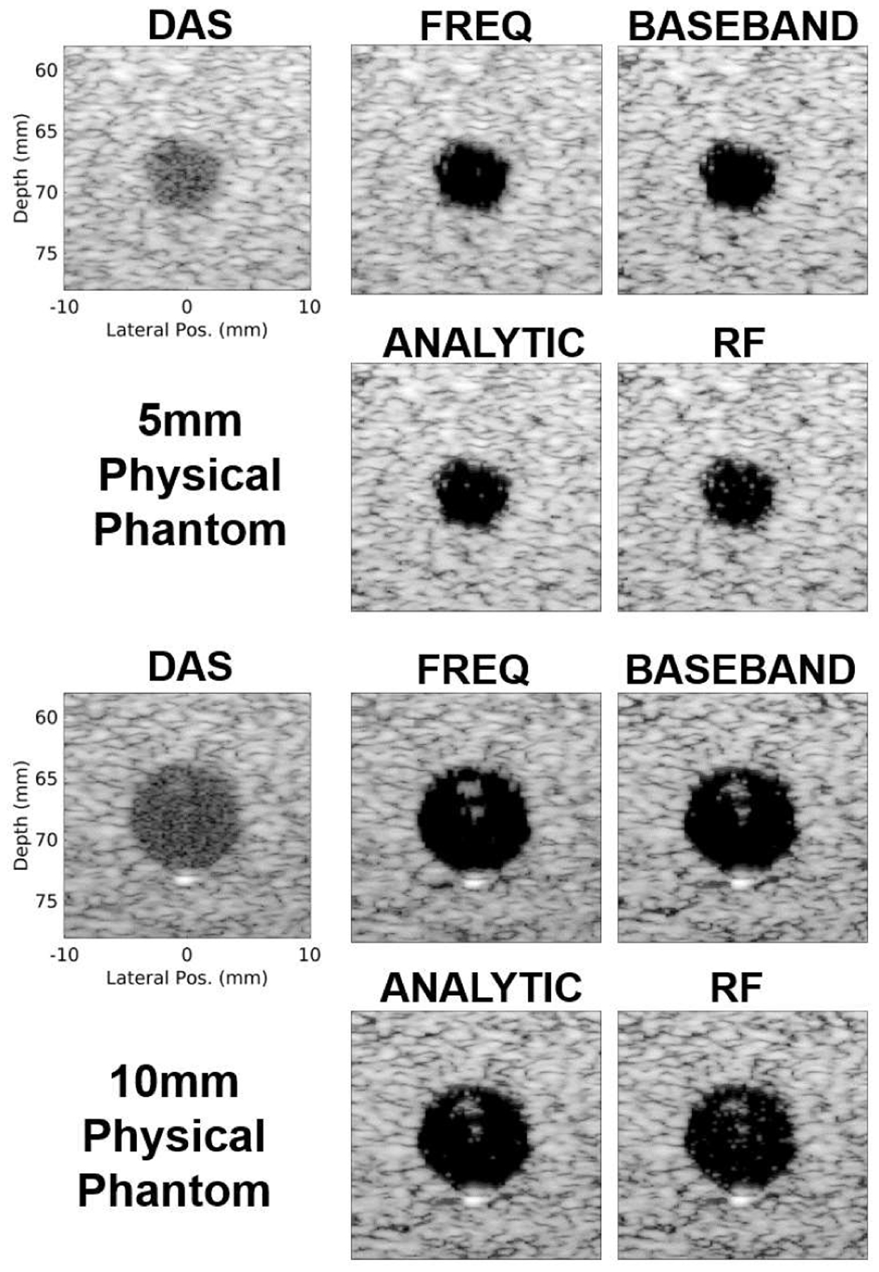
Qualitative results are shown for experiment 3 (i.e., input domain generalization to physical phantom data). B-mode images of example 5mm (top) and 10mm (bottom) cyst physical phantom realizations beamformed using DAS and DNNs for each domain type. For each DNN case, the beamformer that used hyperparameters indicated in Table IV was used to make each image. All images are scaled to individual maximums and a 60dB dynamic range.

D. Input Domain Comparison: Generalization to In Vivo Data

Figs. 11 and 12 demonstrate that, similar to the physical phantom data, the time domain DNNs are able to generalize to in vivo liver data and are able to produce similar image quality compared to the frequency domain DNNs. Fig. 11 shows box plots for which the median value for each method is the central mark in each box. The 25th and 75th percentiles are the bottom and top edges of each box, respectively. The bars extending from each box indicate the minimums and maximums, and outliers are marked in red. These results further support that the time domain implementations are generally robust. However, unlike the above experiments, none of the DNN approaches are able to achieve CNR or SNRs improvements in vivo compared to DAS when using the selected models with hyperparameters indicated in Table IV. This result is supported qualitatively in the top row of Fig. 12. CR improvements are apparent in these images compared to DAS for each DNN beamformer, but speckle dropout is also prevalent, resulting in low CNR and SNRs. Although the selected models perform poorly on in vivo data, other models were able to outperform DAS, as shown quantitatively in the right column of Fig. 11 and qualitatively in the bottom row of Fig. 12. This suggests that the problem with generalization to in vivo data is how models are selected as opposed to general DNN performance. Although it is possible to exhaustively test each model on in vivo test data, it is impractical and generally poor practice. Therefore, a better in vivo model selection approach is necessary.

Fig. 11.

Quantitative results are shown for experiment 4 (i.e., input domain generalization to in vivo data). Box plots display image quality improvements compared to DAS for each domain type computed on in vivo liver data. Results are shown for the selected DNN models with hyperparameters indicated in Table IV (left) and the models that prodcued best possible CNR for each case (right).

Fig. 12.

Qualitative results are shown for experiment 4 (i.e., input domain generalization to in vivo data). B-mode images of an example in vivo liver realization beamformed using DAS, the selected DNN models (top) chosen as the models that produced the best CNR on simulated test data, and the best in vivo models that produced the highest in vivo CNR (bottom). For each selected DNN case (top), the beamformer that used hyperparameters indicated in Table IV was used to generate each B-mode image. Example regions of interest used to compute image quality metrics are displayed on the DAS image in red. CNR and CR values are indicated on each image. Images are scaled to individual maximums and a 60dB dynamic range.

E. CNR Regularization: Model Evaluation and Selection

The model hyperparameters selected for the above experiments produced beamformers that perform well for simulated and physical phantom anechoic cysts. However, when generalizing to a more variable in vivo field of view, those beamformers do not perform as well in terms of CNR and SNRs, as demonstrated in Figs. 11 and 12. Despite this discrepancy, the time domain approaches, especially the time analytic, consistently perform similarly to the frequency domain DNNs. Based on this result in addition to the simplified network architecture, the time analytic approach was used to further explore improvements in model selection using CNR regularization.

The teal dots in Figs. 13(a) and 13(b) represent different time analytic beamformers without CNR regularization and demonstrate the decorrelation between (1) training validation loss and simulation CNR and (2) training simulation CNR and in vivo test CNR, respectively. Based on these plots, CNR improvements compared to DAS are achieved with the time analytic DNN beamformers without CNR regularization. However, the beamformer that produces the highest simulated training CNR counter-intuitively has one of the highest training validation losses and also produces low in vivo CNR. When using the original model selection approach based on simulated CNR, the hyperparameters for the selected model without CNR regularization are the same as those in Table IV with the exception of the batch size which was set to 5,496 for this study. Because of the different batch size and also the random initialized weights for training the separate networks, the image quality metrics are different than those reported in Section III-D for the time analytic in vivo data. Additionally, because of the different regions of interest used to compute CNR during training, as depicted in Fig. 3, the simulated CNR values are also different than the simulated CNR values reported in Section III-A.

Fig. 13.

Quantitative results are shown for experiment 5 (i.e., CNR regularization model evaluation and selection). (a) Average (n = 4) CNR computed on simulated training validation anechoic cyst data vs. training validation loss is shown for each normal DNN beamformer (teal) and CNR-regularized DNN beamformer (pink). Average simulated DAS CNR is indicated by the black dashed line. (b) Average (n = 4) CNR computed on simulated training validation anehcoic cyst data vs. average CNR (n = 15) computed on in vivo test data is shown for each normal DNN beamformer (teal) and CNR-regularized beamformer (pink). Average in vivo DAS CNR is indicated by the black dashed line. Each dot in (a) and (b) represents a different set of hyperparameters used to train each model. The models chosen for each case (i.e., without and with CNR regularization) are indicated with gold outlines. Time analytic single input approach was used for all of the beamformers in these plots. (c) Validation loss per epoch for the selected models is shown for DNN and CNR-DNN. (d) CNR computed on simulated validation training data is shown for each epoch for the selected models. (e) Average CNR and CR computed on simulated validation training data using the selected CNR-DNN model with different λ values.

In contrast to the data without CNR regularization, CNR-regularized DNNs address the discrepancy in model selection, as shown by the pink dots in Figs. 13(a) and 13(b) which represent different time analytic beamformers with CNR regularization. Based on these results, when CNR regularization is used, the model selected based on simulated CNR also converged to low training validation loss and produced high CNR in vivo. The selected CNR-regularized DNN hyperparameters are indicated in Table V. Overall, CNR regularization resulted in correlation values of −0.73 between training validation loss and simulated CNR and 0.07 between simulated and in vivo CNR, compared to 0.10 and −0.28, respectively, without CNR regularization. These results are consistent with our two hypotheses for this experiment: CNR regularization resulted in (1) higher negative correlation between training validation loss and simulated CNR and (2) higher positive correlation between simulated and in vivo CNR.

TABLE V.

Optimal hyperparameters based on simulated anechoic cyst training CNR for CNR regularized DNN beamforming

Hyperparameter	Value
Batch Size	5496
Number of Hidden Layers	6
Layer Width	638
Input Gaussian Noise	False
Input Dropout Probability	0.3
Hidden Node Dropout Probability	0.2
Batch Norm	True
Loss Function	L2
Weight Decay	0

Apart from better model correlation, CNR regularization noticeably improves simulated CNR, as shown by the separation between teal and pink dots in Figs. 13(a) and 13(b). Training progression of validation loss and simulated validation CNR are also shown for the selected models in Figs. 13(c) and (d), respectively. These plots demonstrate that the CNR-regularized DNN beamformers produce similar loss curves to the DNN beamformer without CNR regularization while also converging to a higher CNR.

Finally, Fig. 13(e) demonstrates that the λ value used to regularize the CNR loss function can be adjusted to achieve higher CNR on simulated validation training data for the selected CNR-DNN model. However, increasing λ to place more emphasis on the CNR loss function results in a substantial drop in CR.

F. CNR Regularization: Generalization to In Vivo Data

Fig. 14 demonstrates qualitative improvements in image quality when using DNN beamforming with CNR regularization compared to conventional DNN or DAS beamforming. Specifically, the CNR regularized DNN reduces the speckle dropout that is seen in the conventional DNN images while maintaining contrast improvements compared to DAS. This result is supported quantitatively for the examples in Fig. 14 as well as on average across the full in vivo test set (n = 15), as reported in Table VI. For the results displayed in Fig. 14 and Table VI, the hyperparameters indicated in Tables IV and V were used to train the selected conventional DNN and CNR regularized DNN, respectively.

Fig. 14.

Qualitative results are shown for experiment 6 (i.e., CNR regularization generalization to in vivo data. B-mode images of example in vivo liver data beamformed using DAS and DNNs with (right) and without (middle) CNR-regularization. Example regions of interest used to compute image quality metrics are displayed on the DAS images in red. CNR and CR values are indicated on each image. Images are scaled to individual maximums and a 60dB dynamic range.

TABLE VI.

Quantitative results are shown for experiment 6 (i.e., CNR regularization generalization to in vivo data). Average improvement in in vivo image quality metrics (n = 15) compared to DAS are displayed for DNN beamforming with and without CNR regularization. Standard deviations are indicated in parenthesis.

Metric	DNN	CNR-DNN
CNR (dB)	−0.67 (±3.31)	0.61 (±2.95)
CR (dB)	14.7 (±4.70)	7.80 (±3.47)
GCNR	0.08 (±0.15)	0.01 (±0.16)
SNRs	−0.57 (±0.29)	−0.33 (±0.26)

IV. Discussion

The results in this work suggest that, although the frequency domain implementations are generally superior, it is possible to simplify DNN architectures by using time domain data and multiple input formats without substantially hindering image quality improvements. This is important because it simplifies the training process which is relevant when implementing training improvements and advancements like the CNR regularization proposed in this work. Additionally, the time domain approaches require less computation before and after network processing, which is ideal when pursuing real-time implementations. However, the traditional frequency domain DNN approach generally outperformed the time domain approaches when generalizing to the data least similar to the training data. For example, the frequency domain DNNs produced the highest overall image quality metrics for the physical phantom data, as shown in Fig. 9. That said, the time domain approaches, especially the baseband and analytic IQ, still outperformed DAS. Considering these conclusions, frequency domain DNNs might be better suited when attempting to generalize to particularly noisy environments, while time domain approaches are more practical for real time or clinical applications.

For the analyses in this work, RF time domain single input DNN performance was consistently worse than the other time domain single input approaches. This suggests that phase is an important feature to include for DNN beamforming. Furthermore, the sample scheme that we used in this work makes it so that adjacent RF depths are about 90 degrees out of phase. Therefore, the importance of phase information for DNN beamforming is also demonstrated by the improved image quality when multiple RF depths are used as input, as demonstrated in Figs. 5 and 6.

Although sampling frequency was kept constant for the analyses in this work, it is worth noting that the baseband IQ data could be downsampled without changing performance. Therefore, although the baseband IQ DNNs performed similarly to the analytic IQ DNNs, the potential for improved computation time with the baseband IQ approach potentially makes it more practical for real time implementations.

As indicated in the results, for the anechoic cyst evaluations, single input models that were trained using the hyperparameters in Table IV produced consistently high CNR for all input domain types. However, when generalizing to in vivo data with several randomly placed cysts and structures, those hyperparameters did not produce the best performing DNNs. Similarly, when implementing the multi-input approaches, those hyperparameters were not optimal and actually were considered outliers for all of the multi-input cases with an input size of 16 axial signals. Also, as mentioned in Section III-A, the multi-input networks produced more outliers compared to the single input networks, with the number of outliers increasing as the input size increased and with the most outliers (11 out of 33) occurring for the frequency domain networks with an input size of 16 axial signals. This indicates that the multi-input approaches are more difficult to train, and future work will aim to investigate if the hyperparameter space can be better adjusted for different input sizes. That said, a minimum success rate of 66% is not unreasonable and suggests that the hyperparameter space chosen is already generally robust.

The results in Section III-E show that CNR-regularization worked as a strategy for addressing the model selection problem and substantially improved the selected model performance for in vivo beamforming. It was reasonable to use the single input time analytic approach for development of this training scheme because of the substantial evidence included in this work that this approach is generally robust. However, the time analytic approach is also easily implemented due to the minimal pre- and post-processing steps as described in Fig. 2. However, it is possible to perform CNR regularization on the other input domain types or the multi-input approaches and these implementations should be considered for future work.

Simulated anechoic cysts were used for training and testing in this work because they provide intuitive and clean ground truth information for training a DNN to successfully suppress off-axis scattering and generalize, as we have demonstrated previously for our frequency domain approaches [29], [31]. Additionally, training with anechoic cysts allowed us to incorporate a theoretical CNR value into our CNR regularization which prevented overestimation of CNR. However, as exemplified in Fig. 13e, training with anechoic cysts to suppress off-axis scattering results in an inherent bias towards CR when minimal weight is used for the CNR regularization. Because of this tradeoff, in addition to CNR translating well to clinical observation [48], it made sense to use CNR for regularization in this work. However, it is plausible that the same tradeoff is not as apparent when training with, say, hypoechoic cysts and that regularizing with CR or GCNR is more effective. Therefore, it is worth investigating in future work if different types of training data and/or different regularization schemes improve network performance and model selection. As part of this work, it would also be interesting to see if there is any benefit to incorporating a combination of image quality metrics into the loss function.

Although the presented results are specific to the fully connected architectures used in this work, we believe there are several conclusions that are relevant for deep learning beamforming efforts in general. Among other efforts that aim to improve ultrasound beamforming beyond state-of-the-art, both RF [26] and IQ time domain implementations [27], [28] have been proposed, but the benefit of using one or the other was unclear. In this work, we have demonstrated a clear benefit to using phase-preserving time domain implementations, as shown in Figs. 5–12, as opposed to RF data alone and hypothesize that this conclusion would hold true for other approaches. Additionally, other groups have demonstrated that their networks are able to generalize to data acquired with different transducers and imaging parameters [24], [27], but the boundaries and limitations of these generalizations are not well understood. The results in Figs. 7 and 8 support these previous conclusions while also providing insight as to what limitations exist when attempting to generalize to different imaging parameters that were not seen during training. For example, Fig. 7 demonstrates that DNNs are likely robust to frequency changes due to depth-dependent attenuation but, although improvements can persist compared to DAS, we hypothesize that image quality will likely be suboptimal (i.e., smaller and/or more variable improvements in CNR, CR, GCNR, and SNRs compared to DAS) when using a pulse with a substantially lower transmit frequency than what was used during training. That said, further studies need to be conducted to test this hypothesis on varied training schemes and architectures. Lastly, in this work, we highlight the challenges associated with selecting network hyperparameters, which is relevant for the field of deep learning in general. These challenges are exacerbated for ultrasound beamforming for which ground truth training information is difficult to obtain in vivo. In this work, we demonstrate that selecting models based on simulation performance can lead to poor performance on in vivo data. Although it is possible to use a hold-out in vivo validation data set for model selection, it would not address, and would likely increase, the discrepancy between training loss and image quality. Therefore, it would be ideal to instead continue to try to tailor training schemes with ground truth physical information that will result in better translation to in vivo performance.

V. Conclusion

In this work, we provide a comprehensive comparison and analysis of data representations that can be used for DNN beamforming. Specifically, we compared frequency domain DNNs to baseband IQ, analytic IQ, and RF time domain implementations with both single and multiple input approaches. Our findings suggest that time domain and multiple input implementations are more robust than we previously assumed and, as they are less computationally and architecturally complex, could be better suited for real-time clinical or commercial applications. Moreover, we propose a CNR regularization scheme to improve model selection for in vivo beamforming. We demonstrate that CNR regularization addresses the discrepancy we previously encountered between network performance on simulations and in vivo data.

References

- [1].Dahl JJ and Sheth NM, “Reverberation clutter from subcutaneous tissue layers: Simulation and in vivo demonstrations,” Ultrasound in medicine & biology, vol. 40, no. 4, pp. 714–726, 2014. [DOI] [PMC free article] [PubMed] [Google Scholar]
- [2].Li P-C and Li M-L, “Adaptive imaging using the generalized coherence factor,” IEEE transactions on ultrasonics, ferroelectrics, and frequency control, vol. 50, no. 2, pp. 128–141, 2003. [DOI] [PubMed] [Google Scholar]
- [3].Camacho J, Parrilla M, and Fritsch C, “Phase coherence imaging,” IEEE transactions on ultrasonics, ferroelectrics, and frequency control, vol. 56, no. 5, pp. 958–974, 2009. [DOI] [PubMed] [Google Scholar]
- [4].Lediju MA, Trahey GE, Byram BC, and Dahl JJ, “Shortlag spatial coherence of backscattered echoes: Imaging characteristics,” IEEE transactions on ultrasonics, ferroelectrics, and frequency control, vol. 58, no. 7, pp. 1377–1388, 2011. [DOI] [PMC free article] [PubMed] [Google Scholar]
- [5].Mann J and Walker W, “A constrained adaptive beamformer for medical ultrasound: Initial results,” in 2002 IEEE Ultrasonics Symposium, 2002. Proceedings, vol. 2. IEEE, 2002, pp. 1807–1810. [Google Scholar]
- [6].Synnevag JF, Austeng A, and Holm S, “Adaptive beamforming applied to medical ultrasound imaging,” IEEE transactions on ultrasonics, ferroelectrics, and frequency control, vol. 54, no. 8, pp. 1606–1613, 2007. [PubMed] [Google Scholar]
- [7].Holfort IK, Gran F, and Jensen JA, “Broadband minimum variance beamforming for ultrasound imaging,” IEEE transactions on ultrasonics, ferroelectrics, and frequency control, vol. 56, no. 2, pp. 314–325, 2009. [DOI] [PubMed] [Google Scholar]
- [8].Byram B and Jakovljevic M, “Ultrasonic multipath and beamforming clutter reduction: a chirp model approach,” IEEE transactions on ultrasonics, ferroelectrics, and frequency control, vol. 61, no. 3, pp. 428–440, 2014. [DOI] [PMC free article] [PubMed] [Google Scholar]
- [9].Byram B, Dei K, Tierney J, and Dumont D, “A model and regularization scheme for ultrasonic beamforming clutter reduction,” IEEE transactions on ultrasonics, ferroelectrics, and frequency control, vol. 62, no. 11, pp. 1913–1927, 2015. [DOI] [PMC free article] [PubMed] [Google Scholar]
- [10].Dei K and Byram B, “The impact of model-based clutter suppression on cluttered, aberrated wavefronts,” IEEE transactions on ultrasonics, ferroelectrics, and frequency control, vol. 64, no. 10, pp. 1450–1464, 2017. [DOI] [PMC free article] [PubMed] [Google Scholar]
- [11].——, “A robust method for ultrasound beamforming in the presence of off-axis clutter and sound speed variation,” Ultrasonics, vol. 89, pp. 34–45, 2018. [DOI] [PMC free article] [PubMed] [Google Scholar]
- [12].Luchies AC and Byram BC, “Deep neural networks for ultrasound beamforming,” IEEE transactions on medical imaging, vol. 37, no. 9, pp. 2010–2021, 2018. [DOI] [PMC free article] [PubMed] [Google Scholar]
- [13].Perdios D, Besson A, Arditi M, and Thiran J-P, “A deep learning approach to ultrasound image recovery,” in 2017 IEEE International Ultrasonics Symposium (IUS). Ieee, 2017, pp. 1–4. [Google Scholar]
- [14].Gasse M, Millioz F, Roux E, Garcia D, Liebgott H, and Friboulet D, “High-quality plane wave compounding using convolutional neural networks,” IEEE transactions on ultrasonics, ferroelectrics, and frequency control, vol. 64, no. 10, pp. 1637–1639, 2017. [DOI] [PubMed] [Google Scholar]
- [15].Zhou Z, Wang Y, Yu J, Guo Y, Guo W, and Qi Y, “High spatial–temporal resolution reconstruction of plane-wave ultrasound images with a multichannel multiscale convolutional neural network,” IEEE transactions on ultrasonics, ferroelectrics, and frequency control, vol. 65, no. 11, pp. 1983–1996, 2018. [DOI] [PubMed] [Google Scholar]
- [16].Yoon YH, Khan S, Huh J, and Ye JC, “Efficient b-mode ultrasound image reconstruction from sub-sampled rf data using deep learning,” IEEE transactions on medical imaging, vol. 38, no. 2, pp. 325–336, 2018. [DOI] [PubMed] [Google Scholar]
- [17].Senouf O, Vedula S, Zurakhov G, Bronstein A, Zibulevsky M, Michailovich O, Adam D, and Blondheim D, “High frame-rate cardiac ultrasound imaging with deep learning,” in Medical Image Computing and Computer Assisted Intervention – MICCAI 2018. Springer International Publishing, 2018, pp. 126–134. [Google Scholar]
- [18].Khan S, Huh J, and Ye JC, “Universal deep beamformer for variable rate ultrasound imaging,” arXiv preprint arXiv:1901.01706, 2019. [Google Scholar]
- [19].——, “Adaptive and compressive beamforming using deep learning for medical ultrasound,” IEEE Transactions on Ultrasonics, Ferroelectrics, and Frequency Control, 2020. [DOI] [PubMed] [Google Scholar]
- [20].Huijben IA, Veeling BS, Janse K, Mischi M, and Van Sloun RJ, “Learning sub-sampling and signal recovery with applications in ultrasound imaging,” IEEE Transactions on Medical Imaging, 2020. [DOI] [PubMed] [Google Scholar]
- [21].Kessler N and Eldar YC, “Deep-learning based adaptive ultrasound imaging from sub-nyquist channel data,” arXiv preprint arXiv:2008.02628, 2020. [DOI] [PubMed] [Google Scholar]
- [22].Strohm H, Rothlübbers S, Eickel K, and Günther M, “Deep learning-based reconstruction of ultrasound images from raw channel data.” International Journal of Computer Assisted Radiology and Surgery, 2020. [DOI] [PMC free article] [PubMed] [Google Scholar]
- [23].Simson W, Göbl R, Paschali M, Krönke M, Scheidhauer K, Weber W, and Navab N, “End-to-end learning-based ultrasound reconstruction,” arXiv preprint arXiv:1904.04696, 2019. [Google Scholar]
- [24].Wiacek A, González E, and Bell MAL, “Coherenet: A deep learninǵ architecture for ultrasound spatial correlation estimation and coherence-based beamforming,” IEEE Transactions on Ultrasonics, Ferroelectrics, and Frequency Control, 2020. [DOI] [PMC free article] [PubMed] [Google Scholar]
- [25].Nair AA, Tran TD, Reiter A, and Bell MAL, “A deep learning based alternative to beamforming ultrasound images,” in 2018 IEEE International Conference on Acoustics, Speech and Signal Processing (ICASSP). IEEE, 2018, pp. 3359–3363. [Google Scholar]
- [26].——, “A generative adversarial neural network for beamforming ultrasound images: Invited presentation,” in 2019 53rd Annual Conference on Information Sciences and Systems (CISS). IEEE, 2019, pp. 1–6. [Google Scholar]
- [27].Nair AA, Washington KN, Tran TD, Reiter A, and Bell MAL, “Deep learning to obtain simultaneous image and segmentation outputs from a single input of raw ultrasound channel data,” IEEE Transactions on Ultrasonics, Ferroelectrics, and Frequency Control, 2020. [DOI] [PMC free article] [PubMed] [Google Scholar]
- [28].Hyun D, Brickson LL, Looby KT, and Dahl JJ, “Beamforming and speckle reduction using neural networks,” IEEE transactions on ultrasonics, ferroelectrics, and frequency control, vol. 66, no. 5, pp. 898–910, 2019. [DOI] [PMC free article] [PubMed] [Google Scholar]
- [29].Luchies AC and Byram BC, “Training improvements for ultrasound beamforming with deep neural networks,” Physics in medicine and biology, vol. 64, 2019. [DOI] [PMC free article] [PubMed] [Google Scholar]
- [30].Zhuang R and Chen J, “Deep learning based minimum variance beamforming for ultrasound imaging,” in Smart Ultrasound Imaging and Perinatal, Preterm and Paediatric Image Analysis. Springer, 2019, pp. 83–91. [Google Scholar]
- [31].Luchies AC and Byram BC, “Assessing the robustness of frequency domain ultrasound beamforming using deep neural networks,” IEEE Transactions on Ultrasonics, Ferroelectrics, and Frequency Control, 2020. [DOI] [PMC free article] [PubMed] [Google Scholar]
- [32].Hornik K, Stinchcombe M, White H et al. , “Multilayer feedforward networks are universal approximators.” Neural networks, vol. 2, no. 5, pp. 359–366, 1989. [Google Scholar]
- [33].Bianchini M and Scarselli F, “On the complexity of neural network classifiers: A comparison between shallow and deep architectures,” IEEE transactions on neural networks and learning systems, vol. 25, no. 8, pp. 1553–1565, 2014. [DOI] [PubMed] [Google Scholar]
- [34].Vienneau E, Luchies A, and Byram B, “An improved training scheme for deep neural network ultrasound beamforming,” in 2019 IEEE International Ultrasonics Symposium (IUS). IEEE, 2019, pp. 568–570. [Google Scholar]
- [35].Nair AA, Gubbi MR, Tran TD, Reiter A, and Bell MAL, “A fully convolutional neural network for beamforming ultrasound images,” in 2018 IEEE International Ultrasonics Symposium (IUS). IEEE, 2018, pp. 1–4. [Google Scholar]
- [36].Nair AA, Tran TD, Reiter A, and Bell MAL, “One-step deep learning approach to ultrasound image formation and image segmentation with a fully convolutional neural network,” in 2019 IEEE International Ultrasonics Symposium (IUS). IEEE, 2019, pp. 1481–1484. [Google Scholar]
- [37].Glasmachers T, “Limits of end-to-end learning,” arXiv preprint arXiv:1704.08305, 2017. [Google Scholar]
- [38].Mallart R and Fink M, “The van cittert–zernike theorem in pulse echo measurements,” The Journal of the Acoustical Society of America, vol. 90, no. 5, pp. 2718–2727, 1991. [Google Scholar]
- [39].Paszke A, Gross S, Chintala S, Chanan G, Yang E, DeVito Z, Lin Z, Desmaison A, Antiga L, and Lerer A, “Automatic differentiation in pytorch,” 2017. [Google Scholar]
- [40].Glorot X, Bordes A, and Bengio Y, “Deep sparse rectifier neural networks,” in Proceedings of the fourteenth international conference on artificial intelligence and statistics, 2011, pp. 315–323. [Google Scholar]
- [41].Kingma DP and Ba J, “Adam: A method for stochastic optimization,” arXiv preprint arXiv:1412.6980, 2014. [Google Scholar]
- [42].Glorot X and Bengio Y, “Understanding the difficulty of training deep feedforward neural networks,” in Proceedings of the thirteenth international conference on artificial intelligence and statistics, 2010, pp. 249–256. [Google Scholar]
- [43].He K, Zhang X, Ren S, and Sun J, “Delving deep into rectifiers: Surpassing human-level performance on imagenet classification,” in Proceedings of the IEEE international conference on computer vision, 2015, pp. 1026–1034. [Google Scholar]
- [44].Wagner RF, “Statistics of speckle in ultrasound b-scans,” IEEE Trans. Sonics & Ultrason, vol. 30, no. 3, pp. 156–163, 1983. [Google Scholar]
- [45].Jensen JA, “Field: A program for simulating ultrasound systems,” Med. Biol. Eng. Comput, vol. 34, pp. 351–353, 1996.8945858 [Google Scholar]
- [46].Demirli R and Saniie J, “Asymmetric gaussian chirplet model for ultrasonic echo analysis,” in 2010 IEEE International Ultrasonics Symposium. IEEE, 2010, pp. 124–128. [Google Scholar]
- [47].Rodriguez-Molares A, Rindal OMH, D’hooge J, Måsøy S-E, Austeng A, Bell MAL, and Torp H, “The generalized contrast-to-noise ratio: a formal definition for lesion detectability,” IEEE Transactions on Ultrasonics, Ferroelectrics, and Frequency Control, vol. 67, no. 4, pp. 745–759, 2019. [DOI] [PMC free article] [PubMed] [Google Scholar]
- [48].Smith SW, Wagner RF, Sandrik JM, and Lopez H, “Low contrast detectability and contrast/detail analysis in medical ultrasound,” IEEE Transactions on Sonics and Ultrasonics, vol. 30, no. 3, pp. 164–173, 1983. [Google Scholar]