Diversity of long-lived intermediates along the binding pathway of Imatinib to Abl kinase revealed by MD simulations

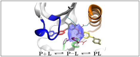
Abstract

Imatinib is a drug for the treatment of Chronic Myeloid Leukemia (CML) and other cancers that works by blocking the catalytic site of pathological constitutively active Abl kinase. While the binding pose is known from X-ray crystallography, the different steps leading to the formation of the complex are not well understood. The results from extensive molecular dynamics simulations show that imatinib can primarily exit the known crystallographic binding pose through the cleft of the binding site or by sliding under the αC helix. Once displaced from the crystallographic binding pose, imatinib becomes trapped in intermediate states. These intermediates are characterized by a high diversity of ligand orientations and conformations, and relaxation timescales within this region may exceed 3–4 ms. Analysis indicates that the metastable intermediate states should be spectroscopically indistinguishable from the crystallographic binding pose, in agreement with tryptophan stopped-flow fluorescence experiments.

Graphical Abstract

1. Introduction

Protein kinases are enzymes that catalyze the transfer of the γ-phosphate of an adenosine triphosphate (ATP) molecule to a tyrosine, serine, or threonine residue of a substrate protein. They form a large family of proteins involved in a wide range of signaling pathways. Ever since the early success of the Abl kinase inhibitor imatinib (Gleevec), tyrosine kinases have been recognized as promising therapeutical targets^1,2. In patients with Chronic Myeloid Leukemia (CML), Abl is expressed as the BCR-Abl fusion protein that is constitutively catalytically active³. Imatinib inhibits BCR-Abl (and a few other aberrant kinases) by blocking its ATP binding site and by locking Abl in a catalytically inactive conformation^1,2. The binding site is located between the N-lobe and the C-lobe of the catalytic domain and it is surrounded by multiple flexible structural elements: the phosphate-positioning loop (P-loop), the activation loop (A-loop), the αC helix and the conserved Asp-Phe-Gly (DFG) motif, that is located at the N-terminal end of the A-loop (see Figure 1).

Figure 1:

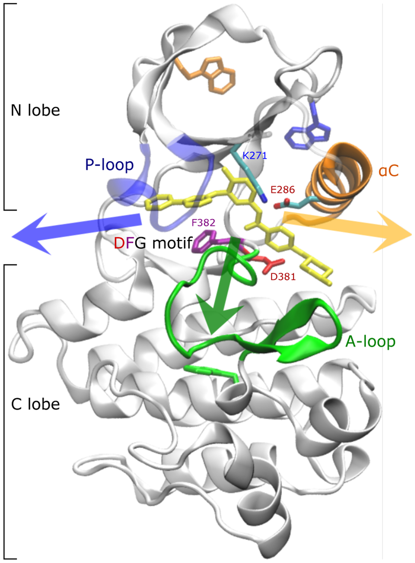
Crystallographic binding mode: imatinib (yellow) bound to the catalytic domain of Abl kinase (pdb id 1IEP⁴). The phosphate-positioning loop or P-loop (blue) as well as salt bridges between the activation loop or A-loop (green) and bf αC helix (orange) cover the binding tunnel at the front. The DFG motif is shown with sticks. Salt bridges involve Asp381 in the DFG motif, Arg386 in the A-loop, Glu286 in the αC helix, and Lys271. The so-called “hydrophobic pocket” is located between the αC helix and the β-sheets in the N-lobe⁵. Tryptophan residues used to monitor the kinetics of binding in fluorescence experiments⁶ are shown as sticks. The three arrows indicate the general direction in which imatinib can leave the binding site. In the following, the orange and green arrows are referred to as the long and short axis, respectively.

The high affinity and specificity of Abl for imatinib raised a number of fundamental questions. For example, while imatinib is a potent inhibitor of Abl, it has a much reduced affinity for c-Src (2400 times), despite the significant sequence identity between the two kinases (47%), particularly at the binding pocket⁷. Based on the X-ray structure of the imatinib-Abl complex showing that the DFG motif was flipped (DFG-out) relative to the more common DFG-in conformation, a “conformational selection” mechanism was proposed to account for the difference in binding affinity⁸. However, this argument was subsequently undermined by additional X-ray structures of c-Src kinase in complex with imatinib and several other inhibitors showing that the DFG-out conformation was also accessible for c-Src^7,9–11. Computational studies showed that the DFG flip is indeed possible for both Abl and c-Src, but the latter is more energetically costly^12–15. Different force fields and computational methodologies indicated that this penalty is on the order of 2–4 kcal/mol^12,14,16, which accounts for the observed difference in binding affinity. Further complicating this “thermodynamic penalty” mechanism, alchemical FEP computations revealed that additional hidden factors (intrinsic affinity, steric clash with P-loop) partly cancel one another to also contribute to the observed affinity of imatinib for Abl and c-Src^13,16,17.

Nevertheless, the issue regarding the molecular origin of the binding specificity of imatinib is not settled. Using kinetic stopped-flow tryptophan fluorescence experiments, Agafonov et al.⁶ showed that imatinib binds via a two-step process represented by the Scheme,

$$\text{P}+\text{L}\rightleftarrows \text{P}-\text{L}\rightleftarrows \text{PL}$$ (1)

where P represents the protein, P-L is the protein-ligand intermediate state, and PL is the strongly bound complex. The first step is a concentration-dependent bimolecular association leading to the formation of a ligand-bound intermediate, and the second step is a slow concentration-independent unimolecular rearrangement. The results were interpreted as evidence of an induced-fit mechanism involving a conformational change of the kinase occurring over a slow timescale after ligand binding, assumed to be at the origin of the high specificity of imatinib for Abl relative to c-Src. However, the structural character of the intermediate state and of the induced-fit step is not known and our understanding of the underlying molecular mechanism is incomplete.

Detailed MD simulations offer a powerful approach to resolve this issue by providing molecular-level information about the binding mechanism of imatinib to Abl and c-Src. In principle, to explain the tryptophan fluorescence experiments, one would need to fully characterize the binding mechanism of the inhibitor with the two kinases, and identify all the critical kinetic steps leading to the formation of the complex. Previous MD studies of the Abl-imatinib system have provided some clues about the binding process. Simulations by Yang et al.¹⁸ indicated that there are two paths for imatinib to enter the binding pocket: either by sliding under the P-loop or by sliding under the αC helix (see Figure 1). Lovera et al.¹⁹ proposed that the intermediate observed in the stopped-flow experiments corresponds to a structure with imatinib bound in the hydrophobic pocket with an imatinib orientation that is reversed with respect to the crystallographic pose (e.g. in PDB structure 2HYY²⁰). The simulation length in these early works was very short (1 ns per trajectory in Yang et al.¹⁸, and 300 ns in total in the metadynamics study by Lovera et al.¹⁹) and we expect that a more thorough sampling will deepen our understanding of the binding process.

Our goal with the present effort is to further our understanding of the binding mechanism by discovering the intermediate conformational states that the Abl-imatinib system visits along the binding/dissociation pathway. For this purpose, we carry out multiple non-equilibrium “pulling” MD simulations, followed by unbiased MD simulations initiated from conformations picked along the pulling trajectories. The simulation data was subsequently analyzed with a VAMPnet²¹ to detect and determine metastable states. The results show that a large number of long-lived intermediate states characterized by a high diversity of ligand orientations and conformations are possible along the binding pathways. Analysis indicates that the set of metastable states generated by the simulations should be spectroscopically indistinguishable from the bound state corresponding to the crystal structure of the imatinib-Abl complex, in agreement with the tryptophan fluorescence experiments of Agafonov et al.⁶

2. Theory and Methods

2.1. MD Setup

The simulated construct consists of residues 235 (Trp) to 498 (Gln) of Abl kinase (numbering scheme of PDB 2HYY²⁰). Initial conformations were taken from PDB crystal structure 2HYY²⁰. Histidines 246, 295, 396, 490 were protonated at their δ site. Histidines 361, 375 were protonated at the ϵ site as in the simulations of Lin and Roux¹⁶. The kinase was solvated with 14577 water molecules (including the crystallographic waters, all of which were kept). We set an ionic strength of 0.15 M by adding 48 potassium ions and 41 chloride ions with Charmm-Gui²². The aqueous concentration of imatinib is roughly 3.8 mM, estimated from the volume occupied by the total number water molecules in the simulation box. For the protein, we use the Charmm-36m forcefield²³. For imatinib we used the previously published parameters¹⁷ that were obtained from quantum computations using the GAAMP software^24,25. MD simulations were run at a temperature of 303.15 K and 1 atm pressure. Simulations were run with repartitioned hydrogen masses in the solute molecules²⁶, allowing an integration time step of 4 fs. In the Anton runs, simulations were run with a time step of 3.2 fs, due to limitations of the M-SHAKE method (and the simultaneous requirement that 100 ns is an integer multiple of the time step, so as to avoid using different time units in different trajectories). All pulling simulations were conducted with the NAMD molecular dynamics code²⁷ and the colvar module²⁸. All unbiased simulations were performed with the Amber GPU code²⁹ and on the Anton supercomputer³⁰. The unbiased non-Anton simulations were run on a small GPU cluster (30 commodity GPUs, GeForce GTX 780) constantly for several months. In-house software was developed to achieve fault-tolerance and to automate failover in cases of GPU overheating and GPU memory errors. Running on a small cluster but for relatively long times allows to generate long trajectories (on the order of 10 μs single trajectory length) which facilitates data analysis.

2.2. Pulling protocol and unbiased trajectories

Unless stated differently in the main text, we applied the following undirected, time dependent pulling potential that acts on the center of mass of imatinib:

$$U(x(t),t)=\frac{k}{2}{\left[\Vert {\text{COM}}_{\text{imat}}(x(t))-c\Vert -vt\right]}^2+U_{\text{res}}(x(t))$$ (2)

where c = COM_imat(x_Xray) is the center of mass of imatinib in the crystal structure 2HYY. k = 100 kcal mol⁻¹A⁻² is the spring constant, v is the pulling velocity v = 6.25 × 10⁻³m/s (in the “slow” simulations) and v = 6.25 × 10⁻²m/s (in the “fast” simulations).

The kinase is restrained in absolute space (lab coordinate system) with the potential U_res(x(t)) that contains a harmonic protein center-of-mass (force constant 200 kcal mol⁻¹A⁻²) and harmonic quaternion restraints (protein rotation restraint, force constant 1000 kcal mol⁻¹)²⁸. In these restraints, the kinase is held by the backbone atoms of its binding pocket. We define the binding pocket as the 85 canonical residues that are shared between kinases and that are reported in van Linden et al.³¹. From the 85 residues, we exclude residues that are in the flexible subdomains (A-loop, αC) which leaves 72 residues. The conformation of the DFG motif was not restrained in any simulation. For some simulations (labeled with “fix” in Table S1), we further restrained the orientation of the αC helix. The force constant for the αC helix was 10 kcal mol⁻¹A⁻².

From the pulling trajectories, a set of 112 initial structures was generated by sampling with uniform time intervals. From all initial structures, long conventional molecular dynamics simulations were run with the Amber GPU²⁹ code. Simulations were terminated if imatinib returned to the crystallographic bound state or dissociated to the the fully unbound state. Only 30 trajectories were terminated, the rest is sampling states were imatinib is trapped in non-crystallographic bound states.

All analysis was done using a combinations of in-house software, VMD³², the MDTraj software³³, the PyEmma software³⁴ and the VAMPnets²¹ package for TensorFlow³⁵.

2.3. Observables for Abl conformational state

To monitor the conformational state of Abl in the presence of imatinib, we use five simple distances that have been shown to well characterize the state of the individual flexible subdomains of kinases (see Table 1)^36,37. As shown by Paul et al.³⁷, the sum d₃ +d₄ can be used to approximately cluster DFG conformations into DFG-in and DFG-out states. Similarly, the sum d₁ + d₂ can be used to distinguish the extended conformation and the kinked conformation of the P-loop. The distance d₆ describes that length of the catalytically important Lys271-Glu286 salt bridge and can therefore be used as an indicator for kinase activation.

Table 1:

Order parameters used for the characterization of Abl kinase sub-domain states in this work and in Meng et al.³⁶, Paul et al.³⁷.

distance number	atoms	structural element
1	Cα-L248 and Cα-Y253	P-loop
2	Cα-G249 and Cα-Q252	P-loop
3	Cγ-D381 Cα-N368	DFG motif
4	Cγ-F382 Cα-I293	DFG motif
5	Cζ-R386 Cδ-E286	αC helix, salt bridge
6	Nζ-K271 Cδ-E286	αC helix, salt bridge

2.4. Visualization of re-binding and dissociating trajectories

To visualize the three groups of trajectories that rebind to the crystallographic state, those that get trapped in intermediate states, and those that fully dissociate, we compute the separating surfaces in the 3-D feature space of the center of mass (COM) position of imatinib. Surfaces are generated with a modified marching cubes algorithm³⁸ as implemented in the scikit-image software³⁹. The input data consists of the center of mass positions of imatinib in all frames of all trajectories. Each trajectory was labeled by the “fate” of the trajectory as determined by the committor like analysis: trajectories that reach zero contacts between imatinib and the kinase are labeled as fully dissociating trajectories. Trajectories where the RMSD between the imatinib atoms position and the imatinib atoms positions in the crystal structure reaches values lower than 2 Å are labeled as rebinding trajectories. All remaining trajectories are labeled as trapped trajectories.

The data points in all trajectories of a given category are discretized on a 3-D grid (grid resolution 3 bins Å⁻¹ for the surface between rebinding trajectories and trapped trajectories and 1 bins Å⁻¹ for the surface between dissociating trajectories and trapped trajectories) after smoothing the points with a Gaussian kernel (kernel size 1/3 Å for the surface between rebinding trajectories and trapped trajectories and 1.5 Å for the surface between dissociating trajectories and trapped trajectories). The resulting grids contain the populations for each category of data points. For each surface, the populations are normalized by the populations in the two respective grid cells, i.e. $p_{i,j,k}=n_{i,j,k}^{(1)}/\left(n_{i,j,k}^{(1)}+n_{i,j,k}^{(2)}\right)$ where i, j, k are the Cartesian grid indices and $n_{i,j,k}^{(1)}$, $n_{i,j,k}^{(2)}$ are the populations of the respective grids. The marching cubes algorithm³⁸ is then applied to the probability grid, so find the isosurface at the reference value p* = 0.5. The marching cubes algorithm computes a set of triangles that represent the isosurface. This procedure alone does not yield the correct dividing surface, but includes patches that lay at the interface of e.g. trapped trajectories and empty grid cells. Consequently, these incorrect parts of the surface are deleted. This deletion is done by first testing whether each triangle separates the two correct volumes, by inspecting the populations grids $n_{i,j,k}^{(1)}$, $n_{i,j,k}^{(2)}$ on both sides of the triangle. The remaining set of triangles is visualized in VMD and superimposed by the crystal structure of Abl kinase domain. For a more rigorous but also more complicated approach (that we do not follow here) see reference⁴⁰.

2.5. Details of VAMPnet analysis

To identify long-lived conformation and to group individual MD snapshots into an expedient number of discrete states, we use a tool from the world of Markov modeling: the VAMPnet²¹. While clustering is not directly part of the computational procedure for determining mechanisms, it helps to organize the data and to objectively define metastable, trapping states that might be responsible for the slow binding of imatinib (See Figure 2).

Figure 2:

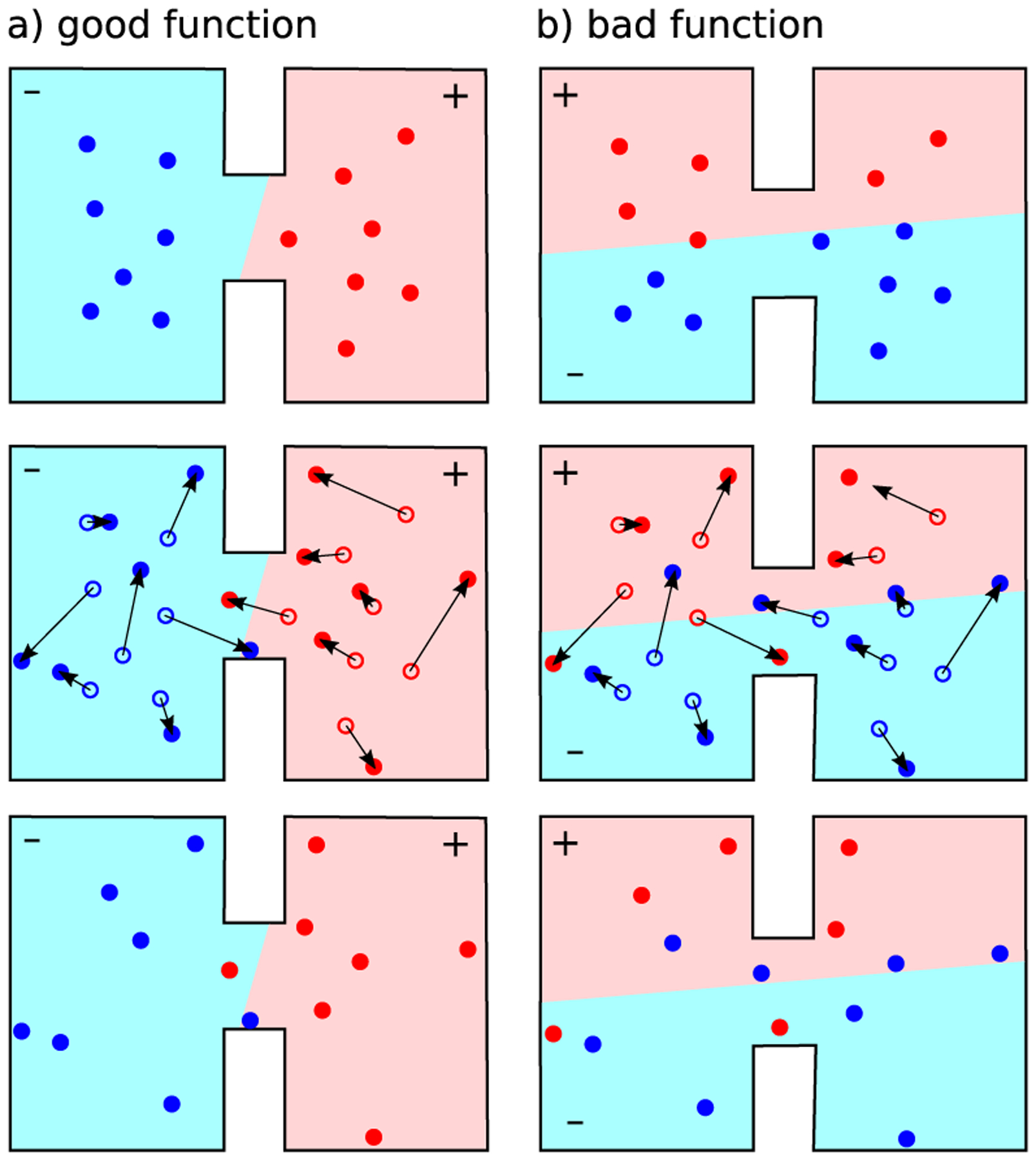
Illustration of variational approach for conformation dynamics: different functions that live in the conformational space are proposed (see (a) for good a example and (b) for a bad example). Functions are ranked by comparing the function’s value at the beginning of time propagation (top row) to the value at the end of the propagation (bottom row).

Like Markov state models, a VAMPnet identifies the long-lived states but does not require the numerous individual (pre-) processing steps of Markov modeling (dimension reduction, clustering, transition matrix estimation, eigendecomposition) thus allowing to obtain results will less manual intervention in the analysis pipeline²¹. VAMPnets combine insights form dynamical operator theory with machine learning to define a differentiable coordinate transformation from conformational space (or alternatively from feature space) to the space of metastable membership functions. The metastable memberships of a conformation express the conformation’s degree of belonging to each of the n metastable states⁴¹. The differentiable transform from conformations to membership functions is optimized with gradient-based techniques, allowing to employ machine learning software packages such as TensorFlow³⁵.

An important component in the VAMPnet is the so-called softmax non-linearity. The softmax is the vector map from ${ℝ}^n$ to [0, 1]ⁿ defined as ${(f(z))}_i=e^{z_i}/{\sum }_k{e}^{z_k}$. For the special case of two metastable states, a softmax transform consists of a pair of Fermi-functions f(w · x + b) and 1 − f(w · x + b) where f(E) = 1/(1 − e^−E), x is a feature vector, and (w, b) are the trainable parameters. Training the neuronal net amounts to optimizing the hyperplane parameters that encode the location of the “Fermi level” (i.e. the hyperplane in feature space/conformational space that belongs with 50% probability to both metastable states) and the “temperature” parameter that encodes the abruptness of the state transition and allows the net to adapt itself to the scaling of the input features. In general, the softmax non-linearity allows to separate more than two states. Still the underlying idea remains the same: half-plane parameters and “temperature” parameters are optimized by following the gradient of an (unsupervised) loss function²¹. Extra non-linearity can be added to the procedure, by stacking additional (non-linear) layers onto the neural net²¹. These allow to deviate from completely planar (linear) hyper-surfaces and equip the separating hyper-surface with curvature and kinks as well as with spatially dependent abruptness parameters.

We trained a shallow and wide VAMPnet comprising only a single soft-max layer on feature trajectories computed from the unbiased molecular dynamics simulations. The input features that go into the VAMPnet to define the metastable states are not the individual atom positions. Instead, the input features can already be grouped in a meaningful way to reduced the input dimension. For the protein, atoms can be grouped into amino acids. For imatinib, there is no such generally agreed upon grouping of atoms, so we defined six groups of atoms (colored differently in Figures 5 and 8). The feature trajectories consist of 1584 = 246*6 minimal reciprocal residue distances between the 246 residues of the simulated Abl construct and the six groups of atoms in imatinib. Computing the reciprocal of minimal distances converts them to smoothed indicator functions that are approximately zero if a contact is broken and non-zero if a contact is formed. Such smooth contacts functions have been proved to preform better for Markov model construction for many molecular systems⁴². Only non-hydrogen atoms were considered in minimal distance computation.

Figure 5:

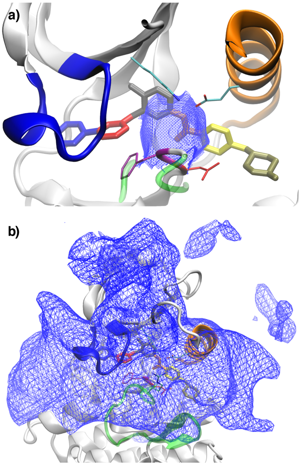
Dividing surfaces in (imatinib) center-of-mass feature space between different classes of trajectories: (a) shows the surface between trajectories that rebind to the crystallographic mode and trajectories that are trapped in intermediate states; (b) shows the dividing surface between trajectories trapped in intermediate states and trajectories that lead to full dissociation. The protein and ligand conformation shown in both figures corresponds to the crystal structure 2HYY. The two surfaces in (a) and (b) delineate the rugged and complex intermediate region of Abl kinase where are located several non-specific long-lived associated states of imatinib. See Theory and Method for additional details on how the surfaces were generated.

Figure 8:

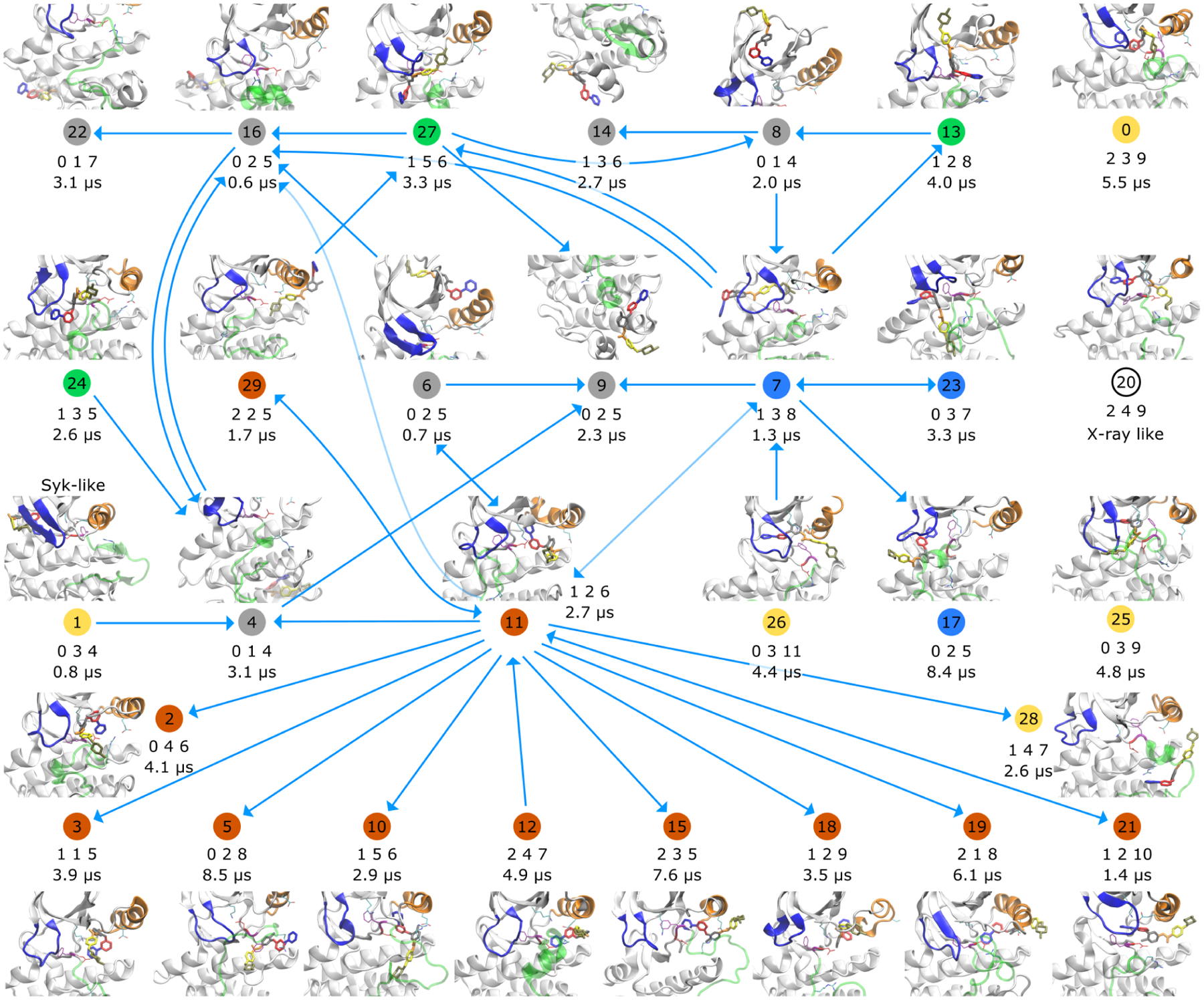
Kinetic network summarizing the unbiased MD simulation data of the Abl-imatinib system. Representative conformations are shown for 30 metastable states, that were identified with a VAMPnet. States that are connected by a transition in the unbiased simulations are connected with an arrow in this plot. Circled numbers below the conformations are the state labels. The color of the disc encodes the broad category of imatinib binding: in orange states imatinib is bound in the hydrophobic pocket; in blue states imatinib is bound under the P-loop; in green states imatinib is bound in front of the cleft; yellow states are DFG-in; in gray states imatinib binds on the surface of Abl. The triple of integers below the state number consists of the number of salt bridges, hydrogen bonds and hydrophobic interactions (in that order) between imatinib and Abl as computed with PLIP⁵¹. Below that, lifetimes or lower bounds on the lifetimes are reported in microseconds. For states that have an outgoing arrow that number is an estimate of the lifetime, otherwise it is a lower bound. Some connections between states (arrows) might be artifacts of the analysis, where VAMP might have merged conformations that should have been separated into different states. See Details of VAMPnet analysis in Theory and Methods for additional information. Magnified versions of all structures are shown in Suppl. Figs. 12 and 13.

The lag time of the VAMPnet was chosen as 10 ns. The neural net was trained with Adam optimizer⁴³ with a fixed learning rate of 10⁻⁴ and using batches consisting of 1000 randomly shuffled transition pairs. The number of epochs was chosen as 60. Multiple repeats were run with different shuffling of the input data (shuffling of transition pairs). 10% of the data (highly correlated to the training data) was selected for cross-validation. Since the sampling of conformational space is so sparse, no independent data can be held out from analysis for cross-validation. Even if, the held out data would be so different form the rest, that it would never confirm the model that was trained on the rest. To do at least some minimal cross-validation, we split the data into two highly correlated sets: a) every tenth frame, starting to count at the zeroth frame b) every 10th frame, starting to count at the fifth frame. Set (a) is used for training while set (b) is used for this “fig leaf” cross-validation.

In almost all runs, the VAMP score²¹ (that is used as the negative loss function) approaches its theoretical maximum which is the number of macrostates. We observe this behavior for different choices of the number of macrostates (15, 20, 30, 40 macrostates). This suggests that there are at least 40 long-lived states that are sampled in our MD data. For the sake of interpretability of the data, we do not cluster with more than 40 macrostates.

2.6. Separation plots

The separation plots analysis is carried out in the following way. Let $M\in {ℝ}^{T\times N}$ be the matrix of metastable memberships for the N metastable states and the T molecular conformations, that was e.g. generated with a VAMPnet. Introduce the linear map $P\in {ℝ}^{N\times 2}$ defined as follows

$$P_{i,1}=\text{sin}\left(\frac{2\pi (i-1)}{N}\right)$$ (3)

$$P_{i,2}=\text{cos}\left(\frac{2\pi (i-1)}{N}\right)$$ (4)

The separation plot is generated by first computing the projected points $S\in {ℝ}^{T\times 2}$ as follows

$$S\text{ = }MP$$ (5)

and subsequently showing them as a scatter plot or 2-D histogram. In the scatter plots, projected memberships for different trajectories are shown with distinct colors. Generalizations of this projection method to other non-circular arrangements are conceivable.

2.7. Modeling tryptophan fluorescence quenching

To relate the results of the MD simulation data to the experimentally measured tryptophan fluorescence data, we recovered the specific total tryptophan fluorescences (amplitudes) from the stopped-flow time traces that were published by Agafonov et al.⁶ The relaxation time traces were modeled with a two-step kinetic model based on Scheme (1). The population dynamics in the induced fit model can be described with the following differential equation

$$\frac{d}{dt}\mathbf{\text{c}}(t)=\mathbf{\text{M}}\mathbf{\text{c}}(t)$$

subject to the initial value condition

$$\mathbf{\text{c}}(0)=\left(\begin{array}{c}{[\text{P}]}_0\\ 0\\ 0\end{array}\right)$$

where

$$\mathbf{\text{M}}=\left(\begin{array}{ccc}-k_{\text{on}}{[\text{L}]}_0& k_{\text{off}}& 0\\ k_{\text{on}}{[\text{L}]}_0& -k_{\text{off}}-k_{\text{conf+}}& k_{\text{conf}-}\\ 0& k_{\text{conf+}}& -k_{\text{conf}-}\end{array}\right)$$

Solving the differential equations, allows to model the fluorescence time traces with the following expression:

$$x\left(t_k\right)={\left(\begin{array}{c}{A}_{\text{U}}\\ A_{\text{I}}\\ A_{\text{X}}\end{array}\right)}^{\top }\mathbf{\text{V}}\left(\begin{array}{ccc}{e}^{{\lambda }_1{t}_k}& 0& 0\\ 0& e^{{\lambda }_2{t}_k}& 0\\ 0& 0& e^{{\lambda }_2{t}_k}\end{array}\right){\mathbf{\text{V}}}^{-1}\left(\begin{array}{c}{[\text{P}]}_0\\ 0\\ 0\end{array}\right)$$ (6)

where λ₁, λ₂, λ₃ are the eigenvalues of M and where V is the matrix of eigenvectors of M. A_U, A_I, A_X are the specific fluorescences of the unbound protein species, the ligand-bound intermediate and the fully bound state respectively. We aim to infer the values of A_U, A_I, A_X including their error bars from the published data.

We modeled the values of the rates (k_on, k_off, k_conf+, k_conf−) with Gaussian priors with parameters set to the respective means and standard deviations reported by Agafonov et al.⁶ The values of the initial concentrations [P]₀ and [L]₀ are modeled with Gaussian priors with parameters set to the nominal ligand and protein concentrations reported in the same publication. We assumed a 10% relative error of the initial concentrations. The time traces from the original publication were digitized with the g3data software and fit with the induced fit model (Eq. 6) using the pymc software package. The initial points in some time traces were excluded, because the fast relaxation appears as a vertical line in the plots in Agafonov et al.⁶ so that the values on the time axis in some of the initial points could not be determined. The missing data was replaced by putting a strong prior on A_U (A_U ∈ [81, 100]) or by adding a virtual data point x(0) = 9.1 to each trace. Each time trace was fit individually.

Distributions of A_U/A_X and A_I/A_X at different concentrations are shown in Figure 3. The plots show that the specific tryptophan fluorescences of the fully bound state and the intermediate state are similar, with the fluorescences of the intermediate being a bit lower than that of the fully bound state.

Figure 3:

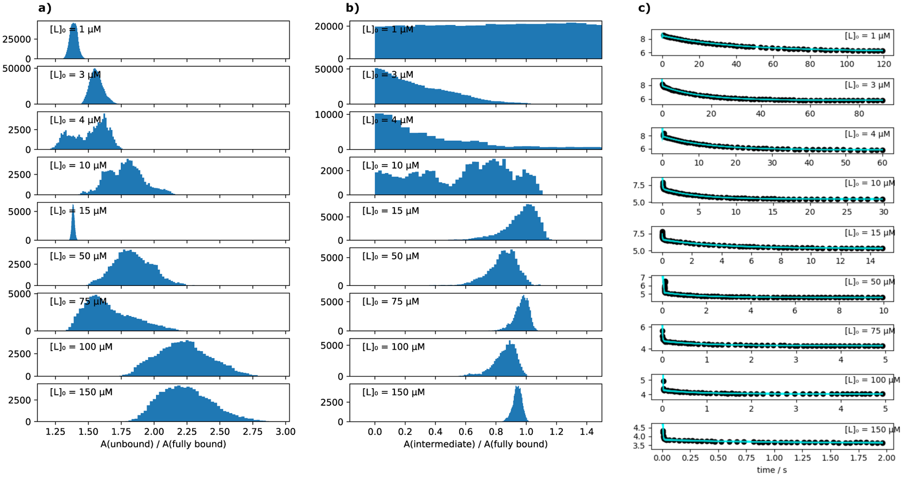
Results of a re-analysis of the tryptophan fluorescence stopped flow data from Agafonov et al.⁶ (a) shows in the form of histograms all values of A_U/A_X that are compatible with the experimental data from Agafonov et al. and contains multiple time traces that were measured at different ligand concentrations [L]₀. We fit each time trace individually (see Modeling tryptophan fluorescence quenching in Theory and Methods for details). (b) shows the corresponding histograms for A_I/A_X. (c) shows the corresponding ensembles of fits to the data (all possible model curves that are compatible with the data).

For the analysis, the solvent-accessible surface area (SASA) for each tryptophan residue was computed with the Shrake-Rupley algorithm⁴⁴ as implemented in the MDTraj software³³. Trp-SASA was computed from three types of data: (i) from a 1.6 μs long MD simulation that was started from the crystal structure 2HYY. (ii) from the set of representative conformations that were sampled from each of the metastable states of the Abl-imatinib system (intermediates and crystal-like state). (iii) from the set of representative conformations that were sampled from the 30 metastable states of apo Abl that were published in Paul et al.³⁷.

3. Results and discussion

3.1. Pulling simulations reveal three main pathways

To escape the crystallographic bound state in the simulation and to generate complex conformations distinct from that state, we performed pulling simulations at different velocities. In the “fast” simulations we pulled 25 Å over 40 ns and in the “slow” simulations over 400 ns. We know that the pathways have to end at the crystallographic pose; we therefore start all pulling simulations from the X-ray structure pdb id 2HYY of human Abl kinase and pull imatinib away from that state (see Theory and Method for details). Our hope with this procedure is to generate mostly conformations that are in some sense close to the crystallographic state, and thus are more likely to fall along the binding/dissociation pathways. Here, we are not especially interested in off-site binding and therefore we do not perform many simulations that start from fully dissociated states. Previous MD studies have shown that the binding-competent DFG-out state is metastable in Abl^14,36,37, we therefore do not prepare simulations with initial conditions in the DFG-in state. (But we also do not prevent the DFG motif from changing conformation during the simulations.)

The results of the pulling are summarized in Figure 4 and Table S1. We find three clusters of broadly different pathways: exit under the P-loop, exit under the αC (i.e. through the hydrophobic pocket) as previously observed by Yang et al.¹⁸, and direct exit though the cleft of the binding site. The pathway through the hydrophobic pocket and through the cleft are observed in two variants each: they can take place with a concerted DFG-out→DFG-in flip or without a flip. Some runs produced unrealistic pathways where imatinib wedges under the αC helix and redirects the pulling force such that the N-lobe is strongly distorted. Such unphysical pathways were more frequent in the fast pulling simulations compared to the slow simulations (see Table S1), and are likely artifacts of the fast pulling. We excluded them from further analysis.

Figure 4:

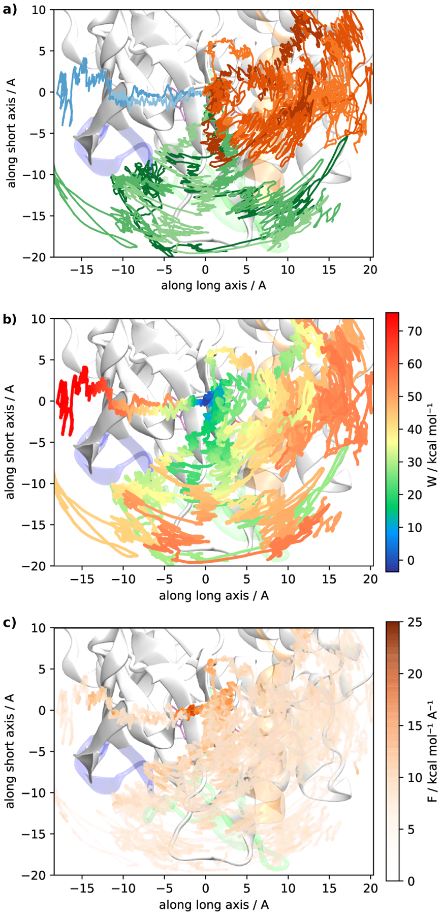
Motion of the center of mass (COM) of the imatinib ligand during the pulling simulations. All three plots show the projection of the COM onto a plane that separates the N and C lobes of the Abl kinase domain along two main directions are referred to as a long and short axis (these two directions corresponding roughly the orange and green arrows in Figure 1, respectively). a) One can discern three clusters of pathways: trajectories where imatinib exits under the αC helix (orange), trajectories where imatinib exits through the cleft (green) and exit in the direction of the P-loop (blue). Blue trajectories were produced with directed pulling while the other trajectories were produced with undirected pulling and imatinib chose the pathway spontaneously. Trajectories were smoothed with a moving average filter with 1 ns window length. The colors in (b) represent the non-equilibrium work at every point along the pulling trajectories. Work was averaged along the path using the same moving average filter (1 ns or 6.25 · 10⁻² Å) as the COM positions. (c) shows the pulling force (averaged with the same filter).

To generate the three types of pathways (under P-loop, under αC, and through the cleft), we ran two different types of pulling simulations: undirected and directed pulling. In the undirected pulling, imatinib is forced to leave the crystallographic binding pose but no direction of motion was imposed (see Pulling protocol in Theory and Methods). Imatinib then spontaneously choses to exit either under the αC or directly through the cleft (with or without DFG-flip). Our undirected pulling failed to produce trajectories where imatinib slides under the P-loop (which had been observed previously with directed pulling¹⁸). We therefore performed additional slow directed pulling slow simulations, that reproduce the exit under the P-loop. Visualizing the pulling force (see Figure 4c) shows that the slope in the beginning of the P-loop pathway is steeper than the slope along the other pathways. The pathway where imatinib squeezes through the cleft without DFG-flip, accumulates the least non-equilibrium work, which is preliminary evidence for its existence (see Table S1). The pathway with the next least non-equilibrium work is the pathway through the hydrophobic pocket (without DFG-flip). Wilson et al.⁴⁵ assumed that the intermediate is DFG-out, while we also observe a DFG-in variant in our pulling simulations.

3.2. Committor-like analysis of intermediate states

Inspection of the pulling trajectories indicates that there are qualitatively different regions in the Abl-imatinib energy landscape. Close to the crystallographic state, it seems that imatinib has to climb out of a deep well in order to leave the binding pose. Close to the fully dissociated state, the force needed to pull imatinib further out becomes relatively small. In between lies a free energy region that appears comparatively rugged (see Figure 4c).

In order to characterize the different regions of the energy landscape, that lie between the crystallographic bound state and the dissociated state, we carried out long unbiased MD simulations that are initiated from different snapshots taken along the pulling simulations. The aggregate trajectory length of all MD data is 529 μs. The unbiased MD simulations are carried out according to a “committor-like” analysis⁴⁶. This means that MD trajectories are terminated whenever they reach the crystallographic bound state or the fully dissociated state. In Figure 5, the ultimate fate of these trajectories is first delineated by two spatial envelopes indicating the starting point of trajectories that rebind to the crystallographic mode (a) and the starting point of trajectories that lead to full dissociation (b).

In Figure 6 we provide a more detailed graphical summary of the committor-like analysis using a projection onto the long and short axis used in Figure 4. Each MD trajectory is represented by a disc. Disc color represents the fate of the trajectory. Cyan means that the trajectory reaches the fully dissociated state. Orange means that imatinib falls back to the crystallographic binding mode. Purple discs represent trajectories that get trapped in intermediate bound states. Disc size represents the time it takes a trajectory to reach its final state (for the cyan and orange discs) or the trajectory length (for the purple discs). Individual trajectory lengths are limited by our computational resources (they range between a few nanoseconds and 30 μs, see Figure S1). The maximum length of 30 μs can therefore only be understood as a lower bound on the lifetimes of the intermediates.

Figure 6:

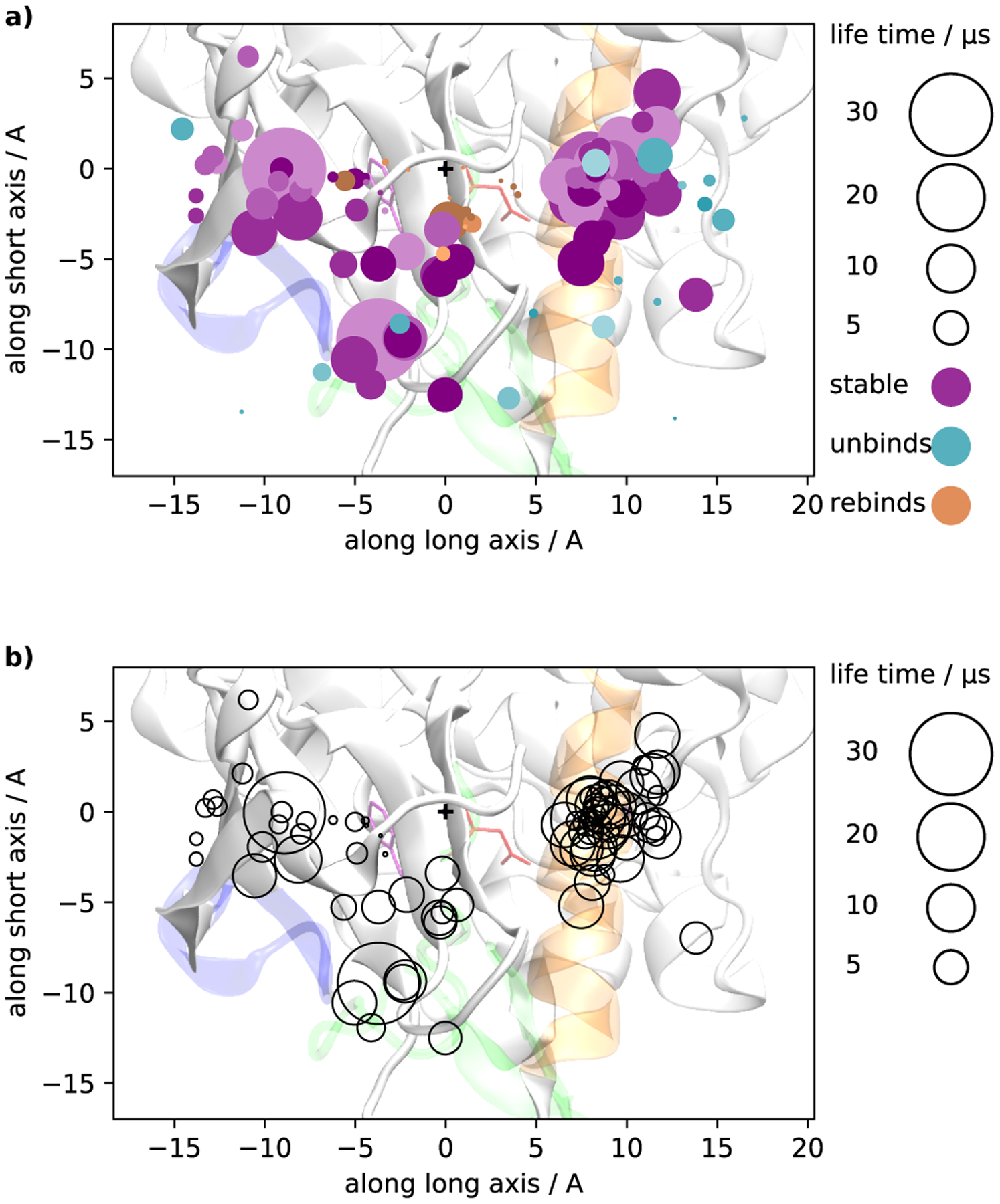
Committor-like analysis reporting the position of imatinib’s center of mass (COM) averaged over the length of each unbiased trajectory. The figure shows the projection of the COM onto a plane that separates the N and C lobes of the Abl kinase domain (same projection as in Figure 4). The plus symbol (+) marks the COM position of the crystallographic bound state. a) Colors indicate the fate of each trajectory: trajectories that reach the fully dissociated state are represented with a cyan disc. Trajectories that reach the X-ray pose are represented with orange discs. All other trajectories are shown as purple discs. Disc sizes represent the time to dissociation or rebinding to the X-ray pose for cyan and orange discs, respectively. In the trajectories that rebind to the X-ray pose, the rebinding time is very short compared to all other processes, therefore the orange discs in (a) are rendered with an area that is magnified by a factor of 10. For purple discs, size corresponds to trajectory length. b) Same as panel (a) showing only the trapped trajectories but without color.

On the basis of Figures 5a and 6, we observe that there is a small region surrounding the X-ray pose where trajectories return quickly to the crystallographic bound state. Conversely, there is a broad region surrounding the active site region where trajectories dissociate fairly rapidly into solvent (Figure 5b). The long-lived intermediate metastable associated states reside within a rugged landscape located in the region between these two surfaces, delineating the configurations rebinding rapidly (Figure 5a) and the configurations rapidly dissociating into solvent (Figure 5b). The trajectories that do not rebind quickly or escape into solvent, become trapped in the intermediate region. We do not observe slow rebinding of these intermediates to the X-ray pose (there are no large orange discs in Figure 6). This indicates that there is a significant bottleneck between the two regions. Figure S2b shows the parts of the pulling trajectories from the X-ray state to the conformation of maximal pulling force. The small region sampled by these trajectories should roughly correspond to the main basin around the crystallographic state.

Visual inspection shows that instead of escaping or rebinding, trajectories in the intermediate region sample new binding modes that we did not observe in the pulling simulations. The modes differ in the location, orientation and conformation of imatinib as well as in the conformation of Abl. Imatinib binds in various poses: in the hydrophobic pocket located between the αC helix and the β-sheets in the N-lobe, under the P-loop, and at the entrance of the cleft. The DFG motif can be in the in or out state.

The observation of long-lived intermediates leads us to the next question: whether some of those intermediates are able to inhibit the catalytic activity of Abl. Since imatinib can move quite far from the crystallographic bound state while still remaining bound to Abl (see Figures 5a and 6), this is a nontrivial question. For most kinases the conformational determinants for catalytic activity are known⁴⁷: the DFG motif needs to be in the in conformation, the salt-bridge between Lys271 and Glu286 needs to be formed (which is facilitated by the inwardly-rotated conformation of the αC helix) and the catalytic spine that involves the residues Asp421, His361, Phe382, Met290, Leu301 needs to be formed⁴⁸. Furthermore, the catalytic site needs to be accessible to ATP and the activation loop must not occlude the catalytic site so that substrate proteins can bind correctly to the kinase. We therefore examined the conformation of the DFG motif and the state of the Lys271-Glu286 salt bridge in all our MD trajectories. In Figure S3 to S7 we show the time-dependent state of the DFG motif and of the salt bridge (for details see Observables for Abl conformational state in Theory and Methods). The time series show that for the majority of trajectories, the DFG motif remains in the out conformation. Notable exceptions are simulations of the so-called “Syk-mode” where imatinib binds under the P-loop as a type I inhibitor similar to the pose observed in a crystal structure of Syk kinase (pdb id 1XBB)⁴⁹. A metastable conformation of Abl resembling that of 1XBB was previously identified in a MSM analysis of apo-Abl³⁷. Three test simulations of this putative Syk-like binding pose for Abl indicate that imatinib would remain stable for a period of time, but then depart from the binding pose on a timescale of about 2 μs. In these simulations, imatinib either remains in state number 1 (see Figure S11, Simulations 96, 98), or leave this pose to go to the superficially bound state number 9 (see Figure S10, Simulations 4).

In some trajectories, we observe an occasional transition of the DFG motif (see Figure S3 to S7 , Simulations 21, 35, 46, 51, 94 ). Since the natural timescale for DFG flipping in many kinases is on the order of milliseconds⁵⁰, we think that the observed DFG flips correspond to the release of tension that has been accumulated by preparing the conformations with pulling simulations. In several trajectories, (Simulations 21, 31, 34, 42, 43, 46, 51, 94) the DFG motif remains in the in state, still the Lys271-Glu286 salt bridge is broken so that the kinase is catalytically inactive (see Figure S3 to S7). Only three trajectories visited the combination of DFG-in with a formed Lys271-Glu286 salt bridge (Simulations 21, 35, 41). However Abl does not become catalytically active in two of these three trajectories, (Simulations 35, 41) since imatinib still occupies the ATP binding pocket. In one trajectory, (Simulation 21) imatinib is initially bound under the P-loop while the DFG motif flips from out to in and imatinib slowly proceeds to dissociation. This latter trajectory captures a stage of activation.

3.3. Orientation of the ligand in the metastable states

To understand how the overall orientation of imatinib changes as it moves along the binding pathway, we map out its polar and azimuthal angles as a function of its position in the plane that separates the N-lobe and the C-lobe. The results are shown in Figure 7.

Figure 7:

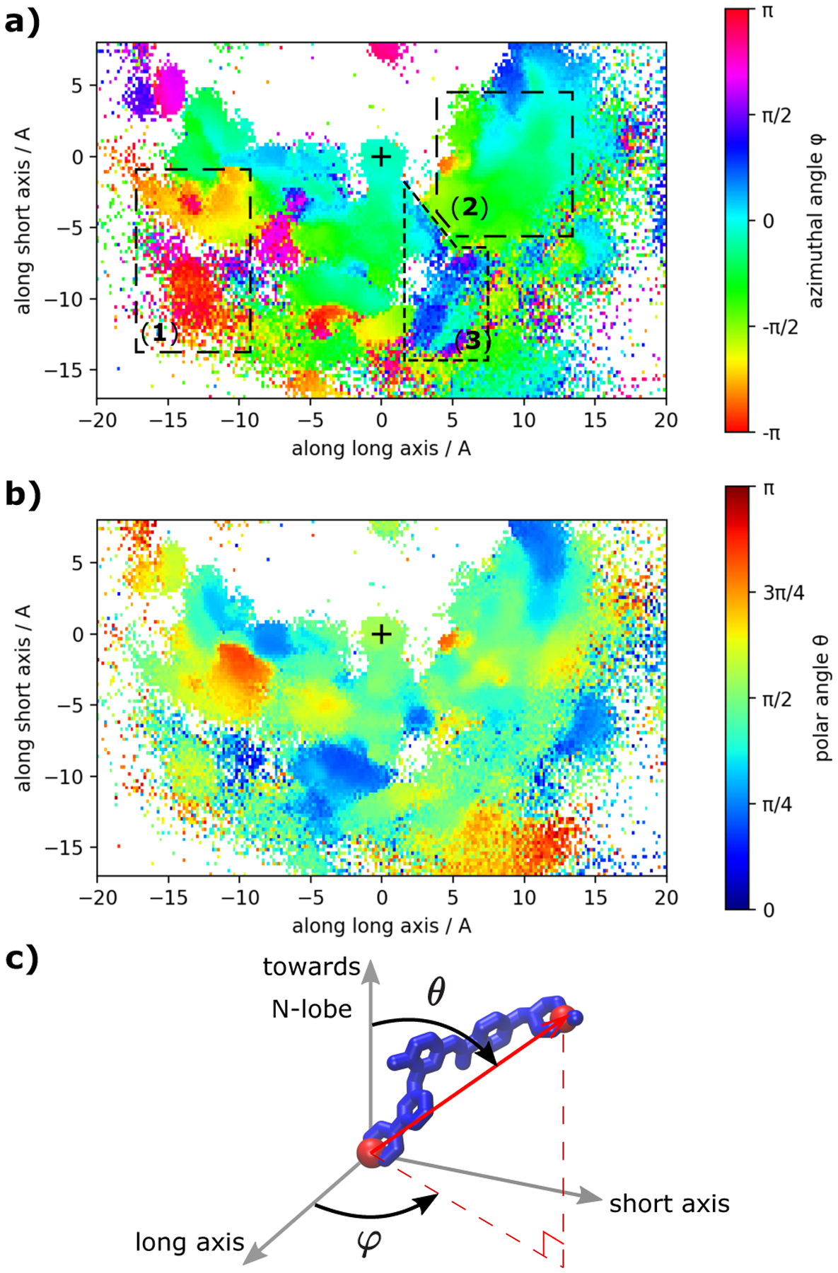
Orientation of imatinib in the different binding poses. In (a) and (b) we visualize the azimuthal angle ϕ and the polar angle θ respectively of the vector through atoms C₈ and N₃₆ that are located at opposite ends of imatinib (red spheres in c). The coordinate system is fixed with respect to the protein and is identical to the system used in Figures. 4, 6). The X-ray like pose is characterized by ϕ ≈ 0 and θ ≈ π/2. The symbol + marks the location of imatinib’s COM in the crystallographic state (similar to pdb id 1HYY). The three main regions are indicated in panel (a).

Keeping in mind that the figure only tracks the orientation of imatinib as a function of its center-of-mass position with respect to the two axes, three main regions are noticeable. In region 1, binding under the P-loop takes place at angles that are different from that in the crystallographic pose. In contrast, in region 2, binding in the hydrophobic pocket and in front of the cleft takes place with an orientation that is quite similar to the crystallographic pose. In region 3, between the crystallographic pose and the hydrophobic pocket pose, there is a well-defined region, where the azimuthal angle changes towards positives values. This might correspond to the barrier where imatinib has to twist in order to transition between these two states. Despite the similar orientations of imatinib in some of the binding modes, interconversion is slow (or even absent in our MD data, e.g. the transition in and out of the crystallographic state) which suggests that the angles are not sufficient to completely explain the binding process.

3.4. Network of metastable intermediate states

We count a total of 59 state-to-state transitions (36 unique pairs of states are connected by at least one transition). However, since many transitions are only observed in one direction with the reverse transition missing in the data, we cannot build an MSM from this MD data. Still, defining the states allows us to estimate lower bounds on the state lifetimes. To systematize the diversity of binding modes and Abl conformations in the MD data, we cluster the data with a single-layer VAMPnet²¹. See Details of VAMPnet analysis in Theory and Methods for additional information.

As the input features for the VAMPnet we use 1584 reciprocal distances between Abl residues and imatinib “pharmacophores”. The VAMPnet assigns conformations to different metastable states²¹, in a similar way as the PCCA+ kinetic clustering algorithm that is used to coarse-grain MSMs^37,52. However, VAMPnets dispense with the geometric clustering step that is used in Markov modeling and therefore allow a much quicker data analysis. From each metastable state, we sample 100 representative conformations for further analysis. The most central conformation of each metastable state is shown in Figure 8, together with the connectivity of the network. The histogram representation in Figure S9 shows that the trajectory data is mostly concentrated in the states that are detected by the VAMPnet (at high state memberships), confirming that the clustering was successful. To further validate the kinetic clustering, we plot in Figure S10 to S11 the metastable assignments that are output by the VAMPnet. The (multivariate) time series representation in these plots confirms that the states are indeed long-lived at the multi-microsecond timescale and that transitions between states are rare events.

Lower lifetime bounds for the individual states are shown below the representative structures in Figure 8 and range between 0.6μs and 8.5μs. Collective lifetimes of an aggregated set of metastable states can be even longer. For instance states 2, 3, 5, 10, 12, 15, 18, 19, and 21 are all states where imatinib binds in the hydrophobic back pocket indicating that the total dwell time in the hydrophobic pocket would be even longer. Results of the clustering reiterate our observation of vastly diverse binding modes, that differ in location, orientation and conformation of imatinib as well as in the conformation of Abl.

It is of interest to consider the relative binding affinity of the different metastable states. While a quantitative assessment based on free energy calculations would be prohibitive, a simple approximation may be sufficient to make important observations. To this end, we compute the number of salt-bridges, of hydrogen bonds and of hydrophobic interactions using the Protein-Ligand Interaction Profiler (PLIP) software⁵¹. The information is provided as three integers in Figure 8. For the crystal structure 2HYY, PLIP reports one salt bridge, 6 hydrogen bonds and 11 hydrophobic contacts. For each metastable state, we compute the corresponding average from 100 representative frames sampled from the state. For the metastable state 20, that contains the crystallographic conformation (2HYY), the average contact numbers are slightly different from the single-conformation numbers (2 salt bridges, 4 hydrogen bonds and 9 hydrophobic contacts). Among the non-crystallographic metastable states, PLIP finds other states with strong polar interactions, in particular state 27 where imatinib is located between the P-loop and the A-loop at the entrance of the cleft, and state 10 where imatinib is partially inside the hydrophobic pocket and partially wedged between the A-loop and the C-lobe. The large number of charged and non-charged interactions in some macrostates strengthens our interpretation that some of the metastable binding poses of imatinib are long-lived. We noted earlier that the overwhelming majority of conformations that are explored by the committor-like analysis are likely to be catalytically inactive. This indicates that non-crystallographic binding of imatinib might have some (minor) contribution to Abl inhibition.

3.5. Overall timescales of the binding process

The transition rates that were extracted from the kinetic model fitted to the stopped-flow tryptophan fluorescence experiments of Agafonov et al.⁶ are 20 s⁻¹ from the intermediate to the fully dissociated state, and 1.5 s⁻¹ from the intermediate state to the final bound state⁶. As the data is primarily of a kinetic nature, it is important to attempt a characterization of the timescales involved in the different aspects of the binding process seen in the computations.

First, we need to determine how association proceeds with imatinib starting in the unbound state. To this end, we run 28 repeats with trajectory lengths ranging between 600 ns and 2 μs (≈ 50 μs of aggregate data) starting with imatinib in the solvent and Abl kinase initialized in the binding-competent DFG-out conformation taken from the crystal structure 2HYY²⁰.

We observe a large number of possible superficial binding poses. These nonspecific binding poses can still be fairly strong, imatinib remaining associated for the entire 2 μs in some trajectories. In two trajectories (unbound-8, unbound-26) imatinib comes close to the entry of the binding tunnel close to the P-loop but does not enter the tunnel. The conformation in trajectory unbound-8 is reminiscent of a reverse Syk-like-mode. In trajectory unbound-21 imatinib attempts to enter the hydrophobic pocket between the αC helix and the β-sheets in the N-lobe (but does not succeed in entering the binding pocket). The region accessible to the ligand starting in the solvent is roughly consistent with the surface delineating the positions of imatinib that rapidly dissociate and escape into solvent (Figure 5b).

These observations regarding the rapid occurrence of nonspecific binding poses are in qualitative agreement with the two-step binding model proposed by Agafonov et al.⁶, which reports a bimolecular binding rate of k_on = 1.5 μM⁻¹s⁻¹ at 5°C. With a simulated aqueous concentration [imatinib] ≈ 3.8 mM of molecules in the MD box, this translates into a mean-first-passage time of 175 μs to the bound state. This estimate is 3.5 times longer than the aggregate simulation data in the unbound state, probably due the remaining long-range interactions between the ligand and protein in the relatively small simulation box.

The timescales of the transitions from the intermediate states to the crystallographic binding pose are considerably more difficult to estimate. The length of the present simulation is on the order of 100 μs and thus a factor of 1000 too short to confirm the experimental data quantitatively. The 30 metastable states shown in Figure 8 show lifetimes τ on the order of 3–4 μs on average. If the network allowed only for a unique connected path through the set of N metastable states, the global timescale for visiting the entire set would go as τN², yielding a timescale on the order of 3–4 ms. While this is certainly a very rough estimate, this naive analysis suggests that long timescales could arise from such a network of metastable states. Importantly, the time to actually reach the X-ray pose which is disconnected from the set of metastable states in Figure 8, is not even considered in this analysis. In this regard, it is noteworthy that, despite the fact that there are multiple pathways leading to the X-ray pose, none of them seems to be downhill on the timescale of the simulation (tens to hundreds of microseconds). On the contrary, the simulations indicate the presence of significant free energy barriers along all pathways. This is in qualitative agreement with the experimental observation of a slow conformational rearrangement in the ligand-protein complex⁶.

Despite the considerable computational resources used here, a total of nearly 600 μs (7.4 μs for the pulling simulations, 529 μs for the committor-like analysis, and 50 μs for the the simulations started with the ligand in solution), a quantitative kinetic characterization of all transitions mapping the binding process cannot achieved on the basis of the current simulations. Nevertheless, the results are generally indicative of the overall very slow timescale that one may anticipate for the binding process. The initial binding starting with the ligand in solution is rapid, while the interconversion from intermediate states to the final crystallographic binding pose is expected to be extremely slow.

3.6. Comparison with fluorescence quenching experiments

The tryptophan fluorescence experiments of Agafonov et al.⁶ revealed that imatinib binds to Abl kinase via a two-step process based on Scheme (1). The first step, P + L → PL, corresponds to a concentration-dependent bimolecular association leading to the formation of a protein-ligand intermediate. The second step, P−L → PL, corresponds to a slow concentration-independent unimolecular rearrangement that ultimately leads this intermediate to the strongly bound protein-ligand complex. Noting that it is this second step that is at the origin of the observed high affinity of imatinib for Abl kinase⁶, the authors interpreted this as evidence for an induced-fit conformational change of the protein kinase that is directly responsible for the binding specificity. The present computational results provide useful information to clarify the interpretation of fluorescence quenching experiments.

Careful numerical analysis of the fluorescence quenching time traces based on the three states of Scheme (1) shows that there are two underlying fluorescence amplitudes (see Modeling tryptophan fluorescence quenching in Theory and Methods for additional information). The fluorescence amplitude of the intermediate and the bound states are very similar whereas the fluorescence amplitude of the apo state is roughly 1.4 times stronger (see Figure 3). To correlate the fluorescence experiments with the computational results, we model the amount of tryptophan quenching on the basis of solvent exposure of tryptophans in the MD simulations⁵³. A comparison of the solvent exposure of the current 30 metastable states of imatinib-bound Abl to the 30 metastable states of apo-Abl from Paul et al.³⁷ shows that the tryptophans in the apo-Abl state are generally more solvent-exposed than in imatinib-bound Abl (see Figure 9). In particular the exposure of the two tryptophans in the N-lobe (W261 and W235) most differs between apo and holo. Among these two the largest the largest difference is for W235, a highly conserved residue within the tyrosine kinase family that is located in a sensitive region near the αC-helix at the boundary of the kinase domain and the N-terminal linker region⁵⁴. In c-Src, it is known that the structure is very sensitive to this residue and that substitution by an alanine (W260A mutant) leads to an increase in basal kinase activity^54–56.

Figure 9:

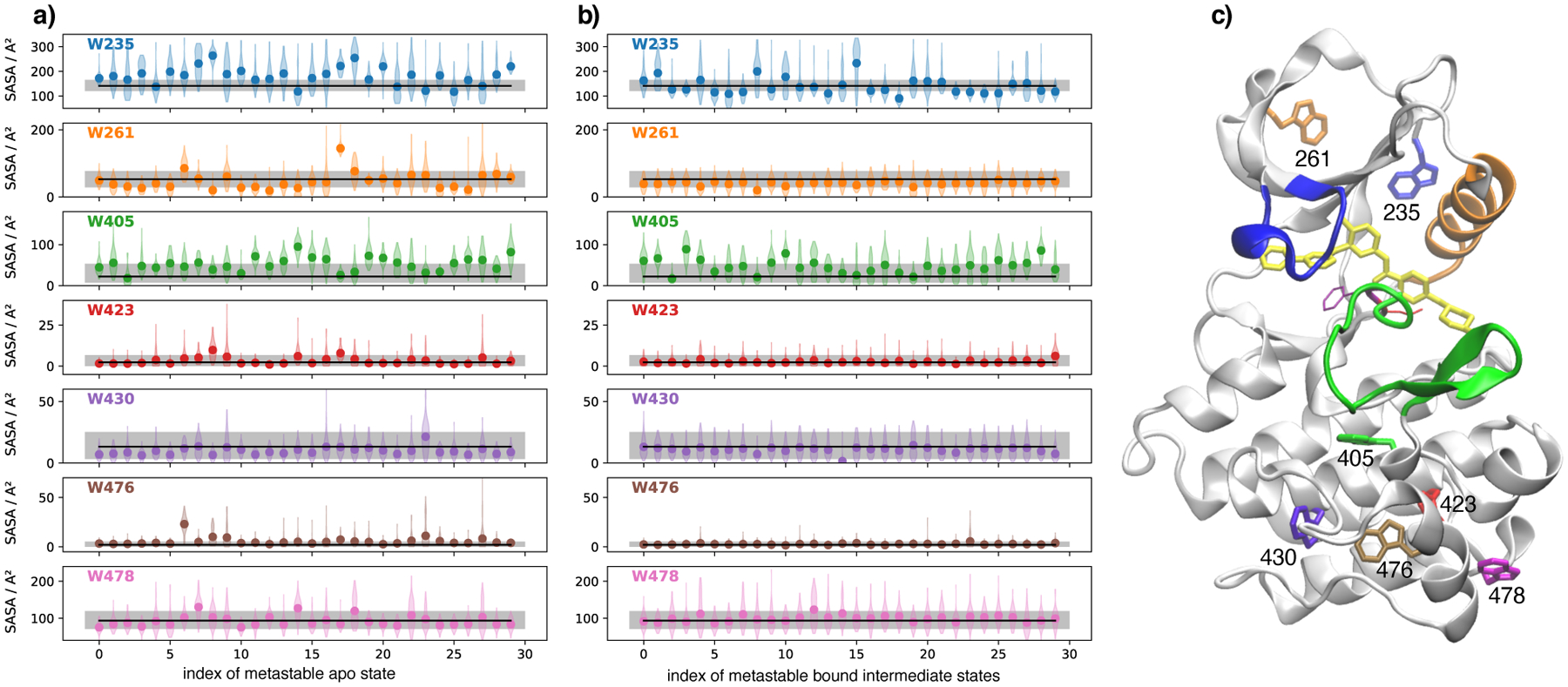
Solvent accessible surface area (SASA) for each tryptophan residue. In (a) Trp-SASA is reported for the 30 metastable states of apo-Abl as defined in Paul et al.³⁷. In (b) the Trp-SASA is shown for each of the 30 metastable states of the Abl-imatinib complex that is studied in the current work. Distribution of the tryptophan SASA within each metastable state is show as a violin plot. Discs mark the means. The black line marks the mean Trp-SASA in a long simulation (1.6 μs) of the Abl-imatinib system started from crystal structure 2HYY. The gray shaded area marks the region between the 5th and 95th percentile of Trp-SASA computed from the same simulation of the crystal structure. (c) shows imatinib-bound Abl with all tryptophan residues labeled.

To further relate the Trp-SASA to the diverse binding modes of imatinib, we show in Figure 10 a 2-D projection of the Trp-SASA onto the same coordinate axes that have been used in Figures 4 and 6. That is, each imatinib COM position is assigned an (averaged) value of the protein Trp-SASA. The 2-D projections show that Trp exposure is similar in all binding modes. The crystallographic binding has a similar Trp-SASA to the intermediate states. This observation is compatible with our numerical analysis of the experimental fluorescence data (see Modeling tryptophan fluorescence quenching in Theory and Methods for for details). In conclusion, this analysis indicates that the set of metastable states generated by the simulations should be spectroscopically indistinguishable from the bound state corresponding to the crystal structure of the imatinib-Abl complex, in agreement with the experiments of Agafonov et al.⁶.

Figure 10:

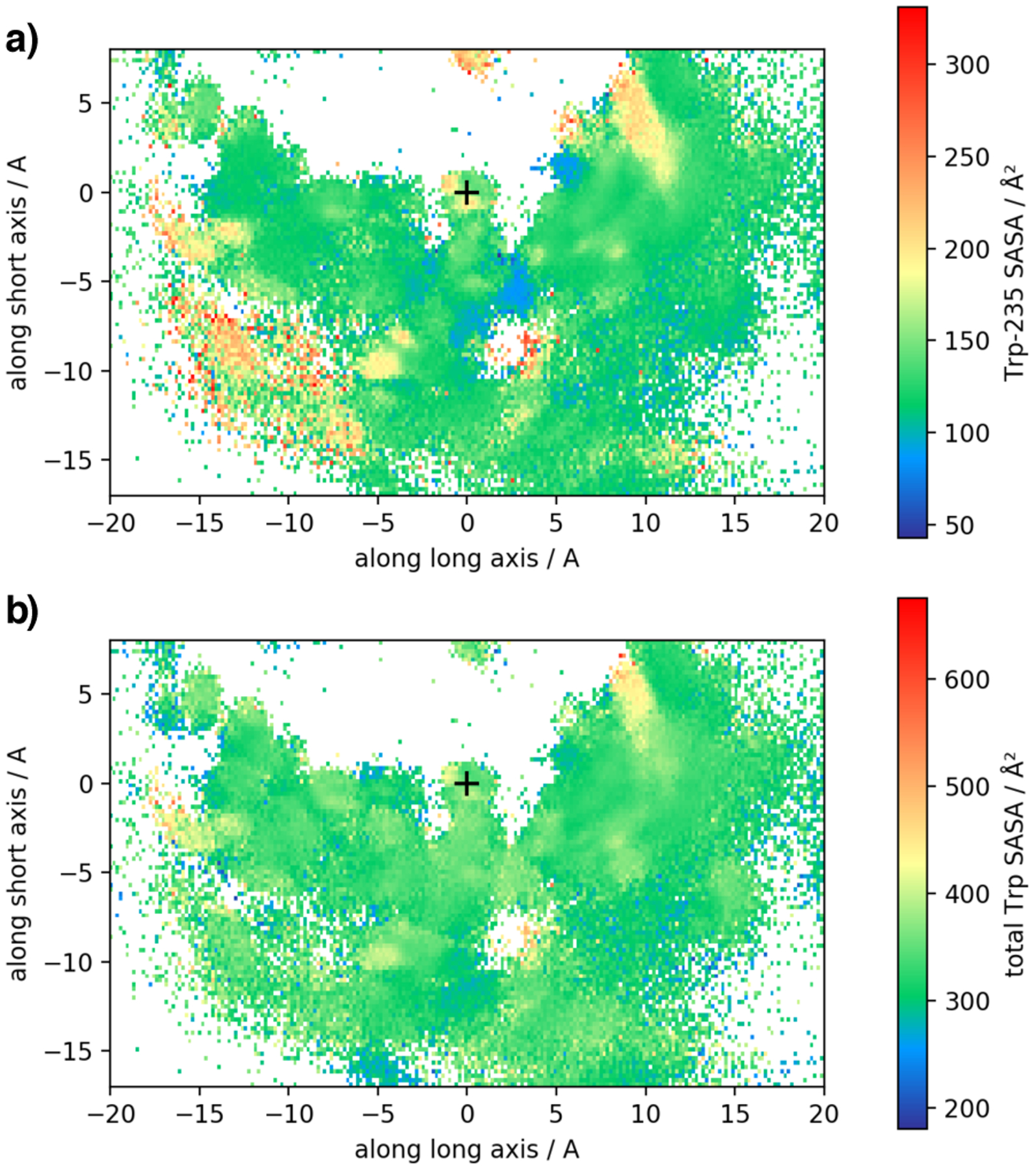
Trp-SASA depending on imatinib location computed from all unbiased trajectories. The coordinates are the same as in Figures 4,6 (imatinib COM in a coordinate system that is fixed w.r.t the protein. The plus (+) symbol marks the location of imatinib’s COM in the crystallographic state. (a) shows the SASA of Trp-235 that is located in the flexible N-terminal liker of the kinase domain. (b) shows the total SASA of all tryptophan side chain in the simulated construct. In agreement with experiment, Trp-SASA does not vary much as the binding pose of imatinib changes.

4. Conclusion

Previously MSM analysis showed that the isolated catalytic domain of Abl is flexible in the absence of ATP and inhibitors^36,37. The present simulations carried out in the presence of the inhibitor show that there exists a large number of metastable states corresponding to non-specific association of imatinib with Abl kinase along two main pathways leading imatinib to the binding pocket: sliding under the αC helix without DFG-flip, and squeezing through the cleft without DFG-flip. These metastable states are located in a highly rugged and complex region of the kinase structure (delineated by the surfaces in Figure 5a and Figure 5b).

While a complete kinetic characterization of all transitions mapping the binding process could not be computationally achieved here, the result from more than 500 μs of aggregate MD data strongly support the notion that the interconversion from the metastable states to the fully bound state is extremely slow. This suggests that the set of metastable binding modes of imatinib could reasonably give rise to the long-lived intermediate state revealed by the tryptophan fluorescence data⁶. In that sense, the picture emerging from the computational analysis is consistent with the actual experimental observation of a slow concentration-independent unimolecular rearrangement leading to the final complex. Nevertheless, describing the slow second step in terms of an induced-fit mechanism warrants some caution.

In the traditional view of the induced-fit mechanism, an initial weakly bound protein-ligand complex induces some conformational changes in the protein that leads to a strongly bound protein-ligand complex. Agafonov et al.⁶ speculated that the slow step detected in the fluorescence experiment is indicative of some conformational change of the kinase that must take place to provide high affinity and specificity. In the present interpretation, it is rather the slow rearrangement of the ligand toward its correct binding pocket from a multitudes of long-lived metastable associated states that underlies the slow step detected in the fluorescence experiment.

Although such a difference may appear to be partly semantic, it is important, in order to avoid confusion, to develop a meaningful physical narrative of the binding process at the molecular-level to help rationally design specific kinase inhibitors. Effectively, a conformation rearrangement of the protein-ligand complex is taking place and is necessary to achieve a strongly bound complex. The picture emerging from the present analysis suggests that the high affinity binding of imatinib with Abl kinase does not involve a major conformational reorganization (induced-fit) of the protein.

What happens is that imatinib encounters a considerable number of non-specific long-lived associated states located in a highly rugged and complex intermediate region before it finds its way in the final high-affinity binding pose. How this picture is altered in the case of c-Src, and its impact on binding specificity, is unknown and shall be the object of future studies.

References

- (1).Druker BJ; Tamura S; Buchdunger E; Ohno S; Segal GM; Fanning S; Zimmermann J; Lydon NB Effects of a selective inhibitor of the Abl tyrosine kinase on the growth of Bcr-Abl positive cells. Nat. Med 1996, 2, 561–566. [DOI] [PubMed] [Google Scholar]
- (2).Mauro MJ; Druker BJ STI571: targeting BCR-Abl as therapy for CML. Oncologist 2001, 6, 233–238. [DOI] [PubMed] [Google Scholar]
- (3).Melo J The diversity of BCR-ABL fusion proteins and their relationship to leukemia phenotype. Blood 1996, 88, 2375–2384. [PubMed] [Google Scholar]
- (4).Nagar B; Bornmann WG; Pellicena P; Schindler T; Veach DR; Miller WT; Clarkson B; Kuriyan J Crystal Structures of the Kinase Domain of c-Abl in Complex with the Small Molecule Inhibitors PD173955 and Imatinib (STI-571). Cancer Res. 2002, 62, 4236–4243. [PubMed] [Google Scholar]
- (5).Roskoski R A historical overview of protein kinases and their targeted small molecule inhibitors. Pharmacol. Res 2015, 100, 1–23. [DOI] [PubMed] [Google Scholar]
- (6).Agafonov RV; Wilson C; Otten R; Buosi V; Kern D Energetic dissection of Gleevec’s selectivity toward human tyrosine kinases. Nat. Struct. Mol. Biol 2014, 21, 848. [DOI] [PMC free article] [PubMed] [Google Scholar]
- (7).Seeliger MA; Nagar B; Frank F; Cao X; Henderson MN; Kuriyan J c-Src Binds to the Cancer Drug Imatinib with an Inactive Abl/c-Kit Conformation and a Distributed Thermodynamic Penalty. Structure 2007, 15, 299–311. [DOI] [PubMed] [Google Scholar]
- (8).Schindler T; Bornmann W; Pellicena P; Miller WT; Clarkson B; Kuriyan J Structural Mechanism for STI-571 Inhibition of Abelson Tyrosine Kinase. Science 2000, 289, 1938–1942. [DOI] [PubMed] [Google Scholar]
- (9).Dar AC; Lopez MS; Shokat KM Small molecule recognition of c-Src via the Imatinib-binding conformation. Chem. Biol 2008, 15, 1015–1022. [DOI] [PMC free article] [PubMed] [Google Scholar]
- (10).Seeliger MA; Ranjitkar P; Kasap C; Shan Y; Shaw DE; Shah NP; Kuriyan J; Maly DJ Equally Potent Inhibition of c-Src and Abl by Compounds that Recognize Inactive Kinase Conformations. Cancer Res. 2009, 69, 2384–2392. [DOI] [PMC free article] [PubMed] [Google Scholar]
- (11).Haldane A; Flynn WF; He P; Vijayan RS; Levy RM Structural propensities of kinase family proteins from a Potts model of residue co-variation. Protein Sci. 2016, 25, 1378–1384. [DOI] [PMC free article] [PubMed] [Google Scholar]
- (12).Lovera S; Sutto L; Boubeva R; Scapozza L; Dölker N; Gervasio FL The different flexibility of c-Src and c-Abl kinases regulates the accessibility of a druggable inactive conformation. J. Am. Chem. Soc 2012, 134, 2496–2499. [DOI] [PubMed] [Google Scholar]
- (13).Lin Y-L; Meng Y; Jiang W; Roux B Explaining why Gleevec is a specific and potent inhibitor of Abl kinase. Proc. Natl. Acad. Sci. USA 2013, 110, 1664–1669. [DOI] [PMC free article] [PubMed] [Google Scholar]
- (14).Meng Y; lin Lin Y; Roux B Computational Study of the “DFG-Flip” Conformational Transition in c-Abl and c-Src Tyrosine Kinases. J. Phys. Chem. B 2015, 119, 1443–1456. [DOI] [PMC free article] [PubMed] [Google Scholar]
- (15).Meng Y; Pond MP; Roux B Tyrosine Kinase Activation and Conformational Flexibility: Lessons from Src-Family Tyrosine Kinases. Accounts Chem. Res 2017, 50, 1193–1201. [DOI] [PMC free article] [PubMed] [Google Scholar]
- (16).Lin Y-L; Roux B Computational Analysis of the Binding Specificity of Gleevec to Abl, c-Kit, Lck, and c-Src Tyrosine Kinases. J. Am. Chem. Soc 2013, 135, 14741–14753. [DOI] [PMC free article] [PubMed] [Google Scholar]
- (17).Lin Y-L; Meng Y; Huang L; Roux B Computational Study of Gleevec and G6G Reveals Molecular Determinants of Kinase Inhibitor Selectivity. J. Am. Chem. Soc 2014, 136, 14753–14762. [DOI] [PMC free article] [PubMed] [Google Scholar]
- (18).Yang L-J; Zou J; Xie H-Z; Li L-L; Wei Y-Q; Yang S-Y Steered Molecular Dynamics Simulations Reveal the Likelier Dissociation Pathway of Imatinib from Its Targeting Kinases c-Kit and Abl. PLOS One 2009, 4, 1–8. [DOI] [PMC free article] [PubMed] [Google Scholar]
- (19).Lovera S; Morando M; Pucheta-Martinez E; Martinez-Torrecuadrada JL; Saladino G; Gervasio FL Towards a Molecular Understanding of the Link between Imatinib Resistance and Kinase Conformational Dynamics. PLOS Comput. Biol 2015, 11, 1–19. [DOI] [PMC free article] [PubMed] [Google Scholar]
- (20).Cowan-Jacob SW; Fendrich G; Floersheimer A; Furet P; Liebetanz J; Rummel G; Rheinberger P; Centeleghe M; Fabbro D; Manley PW Structural biology contributions to the discovery of drugs to treat chronic myelogenous leukaemia. Acta Crystallogr. D 2007, 63, 80–93. [DOI] [PMC free article] [PubMed] [Google Scholar]
- (21).Mardt A; Pasquali L; Wu H; Noé F VAMPnets for deep learning of molecular kinetics. Nat. Commun 2018, 9, 5. [DOI] [PMC free article] [PubMed] [Google Scholar]
- (22).Jo S; Jiang W; Lee HS; Roux B; Im W CHARMM-GUI Ligand Binder for Absolute Binding Free Energy Calculations and Its Application. J. Chem. Inf. Model 2013, 53, 267–277. [DOI] [PMC free article] [PubMed] [Google Scholar]
- (23).Huang J; Rauscher S; Nawrocki G; Ran T; Feig M; de Groot BL; Grub-müller H; MacKerell AD Jr CHARMM36m: an improved force field for folded and intrinsically disordered proteins. Nat. Methods 2016, 14, 71. [DOI] [PMC free article] [PubMed] [Google Scholar]
- (24).Huang L; Roux B Automated Force Field Parameterization for Nonpolarizable and Polarizable Atomic Models Based on Ab Initio Target Data. J. Chem. Theory Comput 2013, 9, 3543–3556. [DOI] [PMC free article] [PubMed] [Google Scholar]
- (25).Boulanger E; Huang L; Rupakheti C; MacKerell AD; Roux B Optimized Lennard-Jones Parameters for Druglike Small Molecules. J. Chem. Theory Comput 2018, 14, 3121–3131. [DOI] [PMC free article] [PubMed] [Google Scholar]
- (26).Hopkins CW; Le Grand S; Walker RC; Roitberg AE Long-Time-Step Molecular Dynamics through Hydrogen Mass Repartitioning. J. Chem. Theory Comput 2015, 11, 1864–1874. [DOI] [PubMed] [Google Scholar]
- (27).Phillips JC; Braun R; Wang W; Gumbart J; Tajkhorshid E; Villa E; Chipot C; Skeel RD; Kalé L; Schulten K Scalable molecular dynamics with NAMD. J. Comput. Chem 2005, 26, 1781–1802. [DOI] [PMC free article] [PubMed] [Google Scholar]
- (28).Fiorin G; Klein ML; Hénin J Using collective variables to drive molecular dynamics simulations. Mol. Phys 2013, 111, 3345–3362. [Google Scholar]
- (29).Case D; Ben-Shalom I; Brozell S; Cerutti D; Cheatham TE I.; Cruzeiro V; Darden T; Duke R; Ghoreishi D; Gilson M; Gohlke H; Goetz A; Greene D; Harris R; Homeyer N; Izadi S; Kovalenko A; Kurtzman T; Lee T; LeGrand S; Li P; Lin C; Liu J; Luchko T; Luo R; Mermelstein D; Merz K; Miao Y; Monard G; Nguyen C; Nguyen H; Omelyan I; Onufriev A; Pan F; Qi R; Roe D; Roitberg A; Sagui C; Schott-Verdugo S; Shen J; Simmerling C; Smith J; Salomon-Ferrer R; Swails J; Walker R; Wang J; Wei H; Wolf R; Wu X; Xiao L; York D; Kollman P AMBER 2018; 2008.
- (30).Shaw DE; Grossman JP; Bank JA; Batson B; Butts JA; Chao JC; Deneroff MM; Dror RO; Even A; Fenton CH; Forte A; Gagliardo J; Gill G; Greskamp B; Ho CR; Ierardi DJ; Iserovich L; Kuskin JS; Larson RH; Layman T; Lee L; Lerer AK; Li C; Killebrew D; Mackenzie KM; Mok SY; Moraes MA; Mueller R; Nociolo LJ; Peticolas JL; Quan T; Ramot D; Salmon JK; Scarpazza DP; Schafer UB; Siddique N; Snyder CW; Spengler J; Tang PTP; Theobald M; Toma H; Towles B; Vitale B; Wang SC; Young C Anton 2: Raising the Bar for Performance and Programmability in a Special-Purpose Molecular Dynamics Supercomputer. SC ‘14: Proceedings of the International Conference for High Performance Computing, Networking, Storage and Analysis. 2014; pp 41–53. [Google Scholar]
- (31).van Linden OPJ; Kooistra AJ; Leurs R; de Esch IJP; de Graaf C KLIFS: A Knowledge-Based Structural Database To Navigate Kinase-Ligand Interaction Space. J. Med. Chem 2014, 57, 249–277. [DOI] [PubMed] [Google Scholar]
- (32).Humphrey W; Dalke A; Schulten K VMD – Visual Molecular Dynamics. J. Mol. Graphics 1996, 14, 33–38. [DOI] [PubMed] [Google Scholar]
- (33).McGibbon RT; Beauchamp KA; Harrigan MP; Klein C; Swails JM; Hernández CX; Schwantes CR; Wang L-P; Lane TJ; Pande VS MDTraj: A Modern Open Library for the Analysis of Molecular Dynamics Trajectories. Biophys. J 2015, 109, 1528–1532. [DOI] [PMC free article] [PubMed] [Google Scholar]
- (34).Scherer MK; Trendelkamp-Schroer B; Paul F; Pérez-Hernández G; Hoffmann M; Plattner N; Wehmeyer C; Prinz J-H; Noé F PyEMMA 2: A Software Package for Estimation, Validation, and Analysis of Markov Models. J. Chem. Theory Comput 2015, 11, 5525–5542. [DOI] [PubMed] [Google Scholar]
- (35).Abadi M; Agarwal A; Barham P; Brevdo E; Chen Z; Citro C; Corrado GS; Davis A; Dean J; Devin M; Ghemawat S; Goodfellow I; Harp A; Irving G; Isard M; Jia Y; Jozefowicz R; Kaiser L; Kudlur M; Levenberg J; Mané D; Monga R; Moore S; Murray D; Olah C; Schuster M; Shlens J; Steiner B; Sutskever I; Talwar K; Tucker P; Vanhoucke V; Vasudevan V; Viégas F; Vinyals O; Warden P; Wattenberg M; Wicke M; Yu Y; Zheng X TensorFlow: Large-Scale Machine Learning on Heterogeneous Systems. 2015; http://tensorflow.org/, Software available from tensorflow.org.
- (36).Meng Y; Gao C; Clawson DK; Atwell S; Russell M; Vieth M; Roux B Predicting the Conformational Variability of Abl Tyrosine Kinase using Molecular Dynamics Simulations and Markov State Models. J. Chem. Theory Comput 2018, 14, 2721–2732. [DOI] [PMC free article] [PubMed] [Google Scholar]
- (37).Paul F; Meng Y; Roux B Identification of druggable kinase target conformations using Markov model metastable states analysis of apo Abl. J. Chem. Theory Comput 2020, 16, 1896–1912. [DOI] [PMC free article] [PubMed] [Google Scholar]
- (38).Lewiner T; Lopes H; Vieira AW; Tavares G Efficient Implementation of Marching Cubes’ Cases with Topological Guarantees. J. Graph. Tools 2003, 8, 1–15. [Google Scholar]
- (39).van der Walt S; Schönberger JL; Nunez-Iglesias J; Boulogne F; Warner JD; Yager N; Gouillart E; Yu T; the scikit-image contributors, scikit-image: image processing in Python. PeerJ 2014, 2, e453. [DOI] [PMC free article] [PubMed] [Google Scholar]
- (40).Hege H-C; Seebass M; Stalling D; Zöckler M A generalized marching cubes algorithm based on non-binary classifications; 1997.
- (41).Röblitz S; Weber M Fuzzy spectral clustering by PCCA+: application to Markov state models and data classification. Adv. Data. Anal. Classif 2013, 7, 147–179. [Google Scholar]
- (42).Scherer MK; Husic BE; Hoffmann M; Paul F; Wu H; Noé F Variational selection of features for molecular kinetics. J. Chem. Phys 2019, 150, 194108. [DOI] [PubMed] [Google Scholar]
- (43).Kingma DP; Ba J Adam: A Method for Stochastic Optimization. arXiv e-prints 2014, arXiv:1412.6980. [Google Scholar]
- (44).Shrake A; Rupley JA Environment and exposure to solvent of protein atoms. Lysozyme and insulin. J. Mol. Biol 1973, 79, 351–371. [DOI] [PubMed] [Google Scholar]
- (45).Wilson C; Agafonov RV; Hoemberger M; Kutter S; Zorba A; Halpin J; Buosi V; Otten R; Waterman D; Theobald DL; Kern D Using ancient protein kinases to unravel a modern cancer drug’s mechanism. Science 2015, 347, 882–886. [DOI] [PMC free article] [PubMed] [Google Scholar]
- (46).Du R; Pande VS; Grosberg AY; Tanaka T; Shakhnovich ES On the transition coordinate for protein folding. J. Chem. Phys 1998, 108, 334–350. [Google Scholar]
- (47).McSkimming DI; Rasheed K; Kannan N Classifying kinase conformations using a machine learning approach. BMC Bioinformatics 2017, 18, 86. [DOI] [PMC free article] [PubMed] [Google Scholar]
- (48).Kornev AP; Haste NM; Taylor SS; Ten Eyck LF Surface comparison of active and inactive protein kinases identifies a conserved activation mechanism. Proc. Natl. Acad. Sci. USA 2006, 103, 17783–17788. [DOI] [PMC free article] [PubMed] [Google Scholar]
- (49).Atwell S; Adams JM; Badger J; Buchanan MD; Feil IK; Froning KJ; Gao X; Hendle J; Keegan K; Leon BC; Müller-Dieckmann HJ; Nienaber VL; Noland BW; Post K; Rajashankar KR; Ramos A; Russell M; Burley SK; Buchanan SG A Novel Mode of Gleevec Binding Is Revealed by the Structure of Spleen Tyrosine Kinase. J. Biol. Chem 2004, 279, 55827–55832. [DOI] [PubMed] [Google Scholar]
- (50).Hanson SM; Georghiou G; Thakur MK; Miller WT; Rest JS; Chodera JD; Seeliger MA What Makes a Kinase Promiscuous for Inhibitors? Cell Chem. Biol 2019, 26, 390–399. [DOI] [PMC free article] [PubMed] [Google Scholar]
- (51).Salentin S; Schreiber S; Haupt VJ; Adasme MF; Schroeder M PLIP: fully automated protein–ligand interaction profiler. Nucleic Acids Res. 2015, 43, W443–W447. [DOI] [PMC free article] [PubMed] [Google Scholar]
- (52).Deuflhard P; Weber M Robust Perron cluster analysis in conformation dynamics. Linear Algebra Appl. 2005, 398, 161–184, Special Issue on Matrices and Mathematical Biology. [Google Scholar]
- (53).Lakowicz JR Principles of Fluorescence Spectroscopy, Second Edition; Springer Science + Business Media: New York, 1999. [Google Scholar]
- (54).Meng Y; Roux B Computational study of the W260A activating mutant of Src tyrosine kinase. Protein Sci. 2016, 25, 219–230. [DOI] [PMC free article] [PubMed] [Google Scholar]
- (55).Gonfloni S; Williams JC; Hattula K; Weijland A; Wierenga RK; Superti-Furga G The role of the linker between the SH2 domain and catalytic domain in the regulation and function of Src. EMBO J. 1997, 16, 7261–7271. [DOI] [PMC free article] [PubMed] [Google Scholar]
- (56).LaFevre-Bernt M; Sicheri F; Pico A; Porter M; Kuriyan J; Miller WT Intramolecular regulatory interactions in the Src family kinase Hck probed by mutagenesis of a conserved tryptophan residue. J. Biol. Chem 1998, 273, 32129–32134. [DOI] [PubMed] [Google Scholar]
Associated Data
This section collects any data citations, data availability statements, or supplementary materials included in this article.