MAGUS: Multiple sequence Alignment using Graph clUStering

Abstract

Motivation

The estimation of large multiple sequence alignments (MSAs) is a basic bioinformatics challenge. Divide-and-conquer is a useful approach that has been shown to improve the scalability and accuracy of MSA estimation in established methods such as SATé and PASTA. In these divide-and-conquer strategies, a sequence dataset is divided into disjoint subsets, alignments are computed on the subsets using base MSA methods (e.g. MAFFT), and then merged together into an alignment on the full dataset.

Results

We present MAGUS, Multiple sequence Alignment using Graph clUStering, a new technique for computing large-scale alignments. MAGUS is similar to PASTA in that it uses nearly the same initial steps (starting tree, similar decomposition strategy, and MAFFT to compute subset alignments), but then merges the subset alignments using the Graph Clustering Merger, a new method for combining disjoint alignments that we present in this study. Our study, on a heterogeneous collection of biological and simulated datasets, shows that MAGUS produces improved accuracy and is faster than PASTA on large datasets, and matches it on smaller datasets.

Availability and implementation

MAGUS: https://github.com/vlasmirnov/MAGUS

Supplementary information

Supplementary data are available at Bioinformatics online.

1 Introduction

Multiple sequence alignment (MSA) is a basic step in many bioinformatic pipelines, but accurate estimation of MSAs on large sequence datasets is challenging, especially for datasets characterized by low sequence identity and high rates of insertions and deletions (indels). Methods that scale to large datasets have been developed (Garriga et al., 2019; Lassmann, 2019; Liu et al., 2009, 2012; Mirarab et al., 2015; Nguyen et al., 2015; Sievers et al., 2011), some of which [e.g. SATé (Liu et al., 2009), SATé-II (Liu et al., 2012), and PASTA (Mirarab et al., 2015)] use divide-and-conquer: they decompose the input sequence dataset into subsets, align each subset using a base alignment method of choice [such as MAFFT (Katoh et al., 2005)], and merge the alignments together (thus treating them as constraints) into an alignment on the full dataset.

There are multiple benefits to divide-and-conquer: scalability to large datasets is one advantage, but improved accuracy is the main draw. The reason for this improvement is that most alignment methods, including top-performing methods like MAFFT, either degrade in accuracy with high rates of evolution and number of sequences, or simply cannot run on large datasets. Divide-and-conquer avoids this by only using these methods on smaller, more closely related subsets of sequences. Because the alignments on such subsets tend to be very accurate, they are treated as constraints. Hence, the accuracy of the final alignment significantly depends on the ability to merge constraint alignments. A tree can then be estimated on the alignment, and then the process can be iterated. By default, SATé-I, SATé-II, and PASTA each run for three iterations.

SATé-II improved on SATé-I by changing the decomposition strategy and PASTA improved on SATé-II by changing the merger step. Each of these changes improved accuracy and scalability, so that PASTA is the state-of-the-art for this family of divide-and-conquer MSA pipelines. Furthermore, UPP (Nguyen et al., 2015), which is designed to produce good alignments in the presence of sequence length heterogeneity, uses PASTA to compute a ‘backbone’ alignment on sequences that are deemed ‘full length’, represents the backbone alignment using an ensemble of profile Hidden Markov Models, and then aligns the remaining sequences to the backbone alignment using the ensemble. Thus, while PASTA (like most other methods) is suitable for datasets without substantial sequence length heterogeneity, it is also used in methods for aligning heterogeneous sequence length datasets.

Here, we present MAGUS, Multiple sequence Alignment using Graph clUStering, a new method to compute large-scale MSAs. MAGUS follows the same initial steps as the first iteration of PASTA, which has the following structure. PASTA computes an alignment using a fast technique (similar to UPP, but using a random selection of sequences for the backbone without consideration for sequence length) and FastTree2 (Price et al., 2010) to compute a tree on the alignment, divides the sequences into disjoint subsets by deleting edges until all the subsets are below the maximum allowed (default 200), computes alignments on the subsets (default MAFFT), and then merges the alignments together [merging pairs of constraint alignments using Opal (Wheeler and Kececioglu, 2007) or Muscle (Edgar, 2004) and then completing the merger using transitivity]. PASTA then computes a tree on the merged alignment using FastTree, and can continue by iterating; by default, PASTA iterates three times. The two main ways that MAGUS differs from PASTA is that it combines the disjoint alignments using the Graph Clustering Merger (i.e. GCM, a new technique we present here) and it does not need to iterate.

We explore MAGUS on a heterogeneous collection of sequence datasets, using both simulated and biological datasets. We find that just one iteration of MAGUS produces more accurate alignments than default PASTA (which uses three iterations) on nearly all datasets we explore; furthermore, MAGUS is faster, since it only needs one iteration.

2 Approach

We begin with a description of the overall strategy, and then discuss the merger step (where we run GCM) in detail.

2.1 Divide-and-conquer strategy

Given an input set S of unaligned sequences

• Step 1: Compute a starting tree for S. In PASTA, 100 sequences are selected at random and aligned; the remaining sequences are added into that alignment, and a tree is computed on the final alignment with FastTree2. In MAGUS, we follow nearly the same technique, except we select 300 sequences whose lengths are within 25% of 75th percentile; the hope is that using longer sequences will reduce the negative impact of short sequences in the input, and using more sequences will improve the accuracy of the starting alignment and tree.

• Step 2: Decompose the sequence dataset into disjoint subsets using the centroid edge decomposition (an option within PASTA), modified to enable the maximum number of subsets to not exceed a specified amount.

• Step 3: Compute alignments on the subsets; we use MAFFT -L-ins-i, the same technique as in PASTA.

• Step 4: Merge the alignments together using GCM, as described in Section 2.2.

As PASTA enables the user to specify algorithmic parameter values for each of these steps, we expose them as well. Our experimental study (see below) presents results for different settings.

2.2 GCM

The main difference between PASTA and MAGUS is the use of GCM, which is the subject of this section. We begin by defining the MSA Merger problem and basic terminology that we will use throughout the article.

The MSA merging problem

• Input: a set $\mathcal{S}=\{S_1,S_2,\dots ,S_k\}$ of MSAs, with S_i an MSA on a set X_i of sequences, $X_i\cap X_j=\varnothing$ if $i\ne j$, and $X={\cup }_i{X}_i$.

• Output: An alignment A on the full set X of sequences that agrees with each of the input alignments; thus, the subalignment of A induced on X_i is identical to S_i (after removing columns containing only gaps).

We will refer to the input set of alignments as ‘constraint alignments,’ to emphasize that the input set is treated as absolute constraints that must be induced by the merged alignment. This is always possible, as the constraint alignments are disjoint. The MSA Merging problem is a straightforward generalization of the well-studied problem of aligning two alignments (Wheeler and Kececioglu, 2007).

 

High-level description of the GCM algorithm. The Graph Clustering Merger (GCM) can be used with nucleotide sequences or with amino acid sequences, and we will describe and test GCM for both types of input; hence, when we say ‘letter’ in a sequence, we allow this to refer to either a nucleotide or an amino acid.

The basic idea of GCM is to merge our constraint alignments by using a library of ‘backbone alignments’ (also called ‘backbones’), which we compute using a selected ‘base MSA method’ (e.g. MAFFT) after sampling representative sequences from each constraint alignment. This approach is related to the MSA methods in Garriga et al. (2019) and Pei and Grishin (2007), each of which merges a set of disjoint alignments by picking one representative sequence from each subset, aligning the set of selected sequences, and then using that new alignment to construct the merged alignment. However, in these methods, exactly one representative sequence per subset is selected and only one ‘backbone’ alignment of representative sequences is computed, so that there is a trivial merged alignment that induces all the subset alignments (Fig. 1).

Fig. 1.

Overview of the GCM algorithm. The input is a set of constraint alignments. (i) We compute a set of backbone alignments with the same number of sequences from each constraint alignment. (ii) We construct the alignment graph. Each node represents a column from a constraint alignment, and weighted edges are derived from homologies inferred in the backbone alignments: thicker lines represent edges with higher weight. (iii) We cluster the alignment graph with MCL. This example shows two violations: the pink-outlined cluster contains two columns from the same (blue) constraint alignment, and there is no valid ordering between the pink- and green-outlined clusters (‘crisscrossing’). (iv) We resolve the violations and produce a valid trace, where each connected component is a column in our final alignment

We depart from these approaches by using more than one backbone, with each having more than one representative sequence from each constraint alignment. The backbone alignments are not constrained to be consistent with the input constraint alignments or with each other. Thus, in GCM there is much more information to use in merging the constraint alignments, but GCM must also deal with conflicts among the backbone and constraint alignments. This use of multiple backbone alignments introduces a whole new layer of challenges compared to these earlier approaches.

Phase 1 computes a library of backbone MSAs that is then used to form a graph, where the vertices correspond to columns within the input constraint MSAs. In keeping with terminology introduced in previous literature (Kececioglu, 1993), we refer to this as the ‘alignment graph’. In Kececioglu (1993), each node in an alignment graph corresponds to one letter from one sequence; however, since we are ‘aligning alignments’, the nodes in our alignment graphs will represent columns of letters from our constraint alignments instead.

Phase 2 clusters the vertices using the Markov Clustering (MCL) technique from Van Dongen (2000), which can be seen as extending the consistency principle in the MSA literature to longer paths in a way that is similar to the technique in Probcons (Do et al., 2005) (please refer to the Supplementary Materials for a more detailed explanation). This results in a set of clusters, each of which is a set of nodes (vertices) in the graph, where the nodes correspond to columns from the constraint alignments. In order for this clustering to define a valid MSA [also called a ‘trace’ in Kececioglu (1993)], for each cluster, the set of associated columns must contain at most one column from any constraint alignment, and it must be possible to order the clusters (from left-to-right) so that there are no ‘crossings’. Hence, the clustering obtained using MCL is only an initial guess for a final ‘trace’ that will give us a legal merged MSA. Consequently, Phase 3 ‘fixes and orders’ the clusters (breaking them apart, if needed) to form a legal MSA.

 

Phase 1: alignment graph construction. We pick a number M of backbone alignments and the target size L per backbone alignment. For each backbone, we randomly select the same number $\lfloor \frac{L}{q}\rfloor$ of sequences from each constraint alignment (where q is the number of constraint alignments), to achieve approximately the desired target size L. We then compute alignments on each backbone set of sequences, thus producing the backbone alignment for that set, and the full set of such backbone alignments forms the backbone library.

Given the backbone library, we construct the ‘alignment graph’, where the vertices correspond to columns (i.e. sites) in the constraint alignments, and edges are derived from the backbone alignments, as we now describe. Given a column j in constraint alignment i, we create vertex S_ij. The edge between vertices S_ij and S_km is included if and only if there is at least one pair of letters from constraint alignment columns S_ij and S_km in the same column in a backbone alignment, and the weight of each such edge is the number of such pairs. Self-loops are retained, as well as edges between different vertices from the same constraint alignment.

 

Phase 2: clustering the graph. The next phase takes the undirected graph G from Phase 1 and partitions the vertices into disjoint clusters. In essence, the purpose of this clustering phase is twofold: (i) to make analysis of the alignment graph more tractable by culling the most weakly supported edges and guiding the construction of the connected components used in our trace (we will call connected components ‘clusters’ from here on out), and (ii) to extend the consistency principle in the multiple sequence alignment literature to longer paths within G, and thus find evidence for homology beyond what can be inferred using just a single third sequence. To perform this clustering, we use the Markov Clustering Algorithm (MCL) (Van Dongen, 2000), which has been used in other problems in bioinformatics [e.g. Li et al. (2003)]. Very briefly, the MCL algorithm tries to capture graph structure through stochastic flow, or the concept that random walks from nodes in a cluster will frequently visit other nodes within the cluster, and rarely visit nodes outside of the cluster. This makes the algorithm a natural choice for the problem at hand. The chief algorithmic parameter in MCL is the inflation factor I, which roughly controls the granularity of the clustering in GCM; the guidelines for choosing I in Von Dongen (2012) suggest four values between 1.4 and 6.

 

Phase 3: clean-up to produce a MSA. The final phase is meant to modify the clustering from the previous step to yield a valid MSA on the full set X of sequences. Our objective is to convert our given set of clusters (connected components) into an ordered set of (possibly different) clusters that form a valid trace. Thus, our task is somewhat similar to the Maximum Weight Trace problem (Kececioglu, 1993). We need our modified set of clusters to satisfy two trace conditions. The first condition is the absence of vertical violations, where some S_ij and S_ik (i.e, two columns from the same constraint alignment) appear together in a cluster (if the clustering algorithm permits overlapping clusters, we must also deal with ‘horizontal’ violations, where the same S_ij appears in more than one cluster). The second condition requires a valid ordering, so that if cluster C comes before cluster $C\prime$, then j < k for every $S_{ij}\in C$ and $S_{ik}\in C\prime$.

Producing this new set of ordered clusters may be achievable just through ordering the original set of clusters (produced in Phase 1), or may require breaking some of the original clusters into two or more parts. Our optimization criterion is to satisfy our requirements using the smallest number of cluster breaks. In other words, we want to retain the integrity of our constraint alignment column matching as much as possible, while teasing a valid trace out of it.

 

Step 1: eliminate cluster violations. We use a greedy approach, which can require breaking clusters apart.

• While violations exist:

  • find the pair $C,S_{ij}$, where C is a cluster and S_ij is a horizontally or vertically violating element in C that has the smallest sum-of-weights between S_ij and the other elements in C (excluding elements from the same constraint alignment).

  • Remove S_ij from C.

The removal of S_ij from the cluster C creates a new singleton cluster. However, singleton clusters (which define single columns in some constraint alignment) are not needed in the next stage, so we will throw out all singleton clusters as we proceed to Step 2. Afterwards, we can reinsert all of the removed columns in their proper locations (and not homologous to any other columns) using the ordering inferred in Step 2.

 

Step 2: order (and possibly fragment) the clusters. With these cluster violations removed, it remains to produce a legal ordering, which can also require breaking clusters apart; this proves to be the most non-trivial component of the algorithm. We formulate this task as a search problem, as we now describe. Each state in the search space is defined by two sets of clusters—a set of clusters that have already been ordered, and a set of remaining unordered clusters. Then, our starting state has an empty ordered set, and all given clusters in the unordered set. An end state is any state with an empty unordered set, meaning that the ordered set contains a complete, valid ordering. This state space has an exponential number of states, and so we do not construct the space explicitly, but rather perform an implicit search from the starting state.

We transition from one state to another by removing a cluster from the unordered set and adding it to the ordered set, if such a move is legal. A cluster X in the unordered set can only be legally moved into the ordered set if it comes strictly ‘before’ every other cluster in the unordered set, element-wise. More formally, we say a move from state $A=(C_1,U_1)$ to $B=(C_2,U_2)$ (where C_i is a set of ordered clusters, and U_i is a set of unordered clusters) is legal if $C_2=C_1\cup \left\{X\right\},U_2=U_1\setminus \left\{X\right\},$ and for all $S_{ij}\in X$, there is no S_ik with k < j belonging to any cluster in U₂. If no legal moves exist, we can transition to another state by breaking one of the unordered clusters apart into two unordered clusters. We want to travel from our starting state to an end state with the smallest number of cluster breaks, which is our measure of distance.

We use the A* algorithm (Hart et al., 1968), a mainstay in pathfinding and graph search applications, to perform the search. A* is an extension of Dijkstra’s algorithm that uses both distance and heuristic measures to guide the search; in our case, the distance measure is simply the size of the ordered set, and the heuristic measure is the size of the unordered set (thus being a lower bound on the remaining distance to travel). This suffices to guarantee that A* will eventually find an optimal path.

Unfortunately, if the given clusters are poorly formed and extensively ‘tangled’, A* will not be able to find an optimal path in a reasonable amount of time. We handle such situations by weighting the heuristic more heavily if progress is not being made [i.e. we switch to Weighted A* (Pearl, 1984)]. This revokes the optimality guarantee, but allows A* to finish more quickly while still finding a reasonable solution.

Once A* finishes, we use the ordering on the clusters to construct the MSA: each cluster contains a set of constraint alignment columns, which we stack together to form a column in the final MSA. The ordering of the columns follows the ordering of the clusters, with gaps added wherever needed. Finally, as noted above, the singleton clusters that were deleted in Step 1 are then inserted into the correct location (defined by the ordering), without making them homologous to any other columns.

 

Runtime complexity. The runtime of MAGUS is dominated by building backbone alignments, which we perform using MAFFT -L-ins-i. This portion is $O(B_n{B}_m^2{B}_l^2)$, where B_n is the number of backbone alignments, B_l is their average length and B_m is the maximum number of sequences in each backbone, and follows from the runtime complexity of MAFFT -L-ins-i (Katoh and Toh, 2008). For additional details, see the Supplementary Materials.

3 Evaluation

 

Overview. We performed three experiments. Experiment 1: We set default algorithmic parameters for a fast variant and a slower variant of MAGUS. Experiment 2: We compare both the fast and slow variants of MAGUS to PASTA run for varying numbers of iterations. Experiment 3: We evaluate the impact of following a PASTA analysis with a single iteration where GCM replaces Opal or Muscle for the alignment merger technique. We perform our evaluation study on the UIUC Campus Cluster. Our analyses are run on nodes with 16 cores, 64 GB of memory and a walltime limit of 4 h (except for 16S.B.ALL, where we use high memory nodes with a limit of 48 h). We provide an overview of representative results here. Commands and additional results are presented in the Supplementary Materials.

 

Datasets. Our evaluation explores a heterogeneous collection of simulated and biological datasets from prior studies, available in public websites [see Smirnov (2020)]. For simulated datasets, we use ten 1000-sequence model conditions from Liu et al. (2009), ranging from 1000M1 (the most difficult) to 1000M4 (relatively easy). We also use 1000 and 10 000-sequence subsets of the RNASim dataset from Mirarab et al. (2015), which evolve under a non-standard model with positive selection. For the biological datasets, we include four large nucleotide datasets from Cannone et al. (2002) and eight protein datasets from BAliBASE (Thompson et al., 1999), where reference alignments are available based on structural features. Since PASTA (and most other alignment methods, other than UPP) is restricted to datasets without sequence length heterogeneity, these biological datasets were first modified to remove the outlier sequences (i.e. the ones that deviate in length from the median by more than 20%). The modified biological datasets range in size from 195 sequences to 24 246 sequences, and vary in the average pairwise sequence identity, percent of the matrix occupied by gaps and other empirical properties. See Table 1 for additional details.

Table 1.

Dataset properties

Dataset	No. of Seqs	Avg. P-dist.	Max P-dist.	% gaps	Seq. length (avg)	Type
Nucleotide datasets
1000M1	1000	0.695	0.769	74	1011	sim NT
1000M2	1000	0.684	0.762	74	1014	sim NT
1000M3	1000	0.660	0.741	63	1008	sim NT
1000M4	1000	0.495	0.606	61	1007	sim NT
1000S1	1000	0.694	0.768	53	1006	sim NT
1000S2	1000	0.693	0.768	35	1005	sim NT
1000S3	1000	0.686	0.763	37	1005	sim NT
1000L1	1000	0.695	0.769	73	1023	sim NT
1000L2	1000	0.696	0.769	58	1018	sim NT
1000L3	1000	0.687	0.763	85	1042	sim NT
RNASim	1000	0.411	0.609	68	1555	sim NT
16S.M	740	0.298	0.694	60	947	bio NT
16S.3	5489	0.307	0.833	77	1505	bio NT
16S.T	5548	0.306	0.901	83	1501	bio NT
16S.B.ALL	24 246	0.208	0.769	73	1444	bio NT
Amino acid datasets
BBA0039	732	0.364	0.918	69	382	bio AA
BBA0067	274	0.779	0.895	56	448	bio AA
BBA0081	195	0.860	0.967	63	578	bio AA
BBA0101	322	0.778	0.899	51	465	bio AA
BBA0117	423	0.750	1.000	46	56	bio AA
BBA0134	370	0.710	1.000	70	458	bio AA
BBA0154	295	0.662	0.850	51	514	bio AA
BBA0190	343	0.697	0.900	56	896	bio AA

Note: We show the number of sequences, average and maximum P-distance (i.e. normalized Hamming distance), average unaligned sequence length, and whether the dataset is simulated or biological. The biological datasets were pre-processed to remove sequences of length more than 20% above or below the median length.

 

Criteria. We use SPFN and SPFP, computed using FastSP (Mirarab and Warnow, 2011). SPFN denotes the Sum-of-Pairs False Negative rate, which is the fraction of pairs of homologous letters in the true alignment that are not aligned in the estimated alignment. SPFP is the corresponding Sum-of-Pairs False Positive rate, the fraction of pairs of aligned letters in the estimated alignment that are not in the true alignment. SPFN and SPFP are related to the SP-Score and Modeler scores (used sometimes in protein alignment evaluation) by the formulae: SP-score = 1-SPFN and Modeler Score = 1-SPFP. Due to space constraints, we show SPFN and SPFP in the supplementary materials, and report their average in the main article.

Runtimes are reported for each process running start-to-finish on a single cluster node, with both PASTA and MAGUS exploiting multi-threading in a similar way (i.e. the MAFFT -L-ins-i runs are parallelized).

4 Results

4.1 Experiment 1: parameter tuning for MAGUS

MAGUS has multiple algorithmic parameters: MCL inflation parameter for GCM, starting tree, number of constraint subsets, number and size of backbone alignments, and whether the backbone alignments are extended to full alignments using HMMER (Eddy, 2020) (see Supplementary Materials). We performed extensive experiments on the 1000M1 model condition to evaluate the impact of how we set these parameters; we excluded one of the 20 replicates as a persistent outlier, and used performance on the other replicates for this experiment. This experiment determined default settings for two modes of MAGUS: a fast version, which does not include the HMM-extension technique, and a slow version that does. Both versions use the same settings for the other parameters: MCL inflation parameter 4, a starting tree that we have developed, 10 backbones of size 200 and divide the input sequence set into 25 subsets for constraint alignment creation. Here we show how changes to these selected parameters impact accuracy and running time. (The results for different inflation factors are provided in the supplementary materials, and are less interesting as they follow a standard recommendation in any event.)

 

Experiment 1(a): varying the size and number of backbone alignments and number of constraint alignments. We vary the number of constraint alignments, and the number and size of our backbones (Fig. 2). We use the MAGUS starting tree and fix the inflation parameter to 4.

Fig. 2.

Experiment 1(a): Exploring the impact of varying the size and number of backbone alignments, and number of constraint alignments. ‘A × B’ indicates MAGUS being run with B backbones of size A in fast mode. Top: The error rates are the average of SPFN and SPFP, and are averaged over the 19 replicates of the 1000M1 model condition. Error bars indicate standard error. The x-axis shows the impact of changing the number of subsets. Bottom: Average running time (in minutes) over the 19 replicates of the 1000M1 model condition. Error bars indicate standard error. The x-axis shows the impact of changing the number of subsets

Note that the best accuracy is obtained using 25 constraint alignments and 15 backbones of size 200 or 300. Given the use of 25 constraint alignments and 15 backbones, there is no difference in accuracy between backbones of size 200 and 300, but that change does impact the running time. However, smaller backbones definitely increase error, and fewer than 10 backbones also increase error noticeably. There is only a small decrease in accuracy when using 10 instead of 15 backbone alignments, and so if running time is considered, the best default setting seems to be 25 constraint alignments and 10 backbones of size 200. If time permits, then 15 or even 20 backbones can be used, and such a setting might reasonably be used on much larger datasets, where the computation of constraint alignments would dominate the runtime anyway.

 

Experiment 1(b): varying the starting tree, number of constraint alignment subsets and HMM-extension. In this experiment we show the impact of the choice of starting tree and the use of HMM-extension (see Supplementary Materials for commands), while allowing the number of constraint alignments to change; all analyses use inflation factor I = 4 and we use 10 backbones of size 200.

There is an advantage in alignment accuracy to using the MAGUS starting tree instead of the PASTA starting tree, and this advantage is present at every number of constraint alignments we examine (Fig. 3). The impact of using the HMM-extension to complete the backbone alignments (‘slow’ mode) is generally positive—improving accuracy with 25 or more constraint alignments and neutral on fewer constraint alignments. However, using the HMM-extension increases the runtime (e.g. the median runtime here increases by as much as 10 min). However, of perhaps greater concern is the high variance in the runtime when using the HMM-extension, which suggests that it may become very computationally expensive to use on large datasets.

Fig. 3.

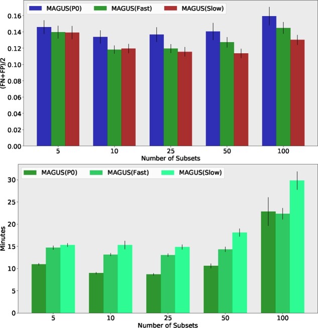
Experiment 1(b): Exploring the impact of starting tree, HMM-extension and subset number on MAGUS on 1000M1. Top: The error rates are the average of SPFN and SPFP, and are averaged over the 19 replicates of the 1000M1 model condition. Error bars indicate standard error. MAGUS(P0) uses the PASTA starting tree instead of the MAGUS starting tree. MAGUS(Slow) uses the HMM-extension. The x-axis shows the impact of changing the number of subsets. Bottom: Average running time (in minutes), averaged over the 19 replicates of the 1000M1 model condition. Error bars indicate standard error. The x-axis shows the impact of changing the number of subsets

4.2 Experiment 2: MAGUS versus PASTA

The central experiment of our study is the comparison between MAGUS and PASTA. MAGUS(Fast) and MAGUS(Slow) differ in the use of the HMM-extension, but otherwise both use 25 constraint alignments and 10 backbones of size 200, and the same starting tree. Of the ten model conditions with 1000 sequences (Fig. 4), both versions of MAGUS have better accuracy on nine conditions and tie with PASTA on one condition. The largest differences are on the hardest model condition, 1000L3, where MAGUS (both versions) leads PASTA by about 6–7% (10–11% versus 17–18%). The difference narrows, but persists, under easier model conditions. The use of MAGUS(Slow) provides an accuracy benefit under the harder model conditions, and otherwise has very similar accuracy as MAGUS(Fast). Moreover, MAGUS(Slow) and MAGUS(Fast) are both much faster than PASTA, generally completing in about half the time (e.g. a reduction from about 40 min for PASTA to about 15 min for MAGUS on 1000M2, and from about 20 min to about 10 min on 1000M3). Lastly, the error bars indicate that MAGUS tends to have noticeably lower variability in its accuracy and runtime than PASTA under the harder model conditions.

Fig. 4.

Experiment 2: MAGUS versus PASTA on the 1000-taxon datasets. Top: The error rates are the average of SPFN and SPFP. The x-axis shows the model condition; each model condition has 1000 sequences. Results are averaged over 20 replicates. Error bars indicate standard error. PASTA and MAGUS were run in default mode. Bottom: Average running time (in minutes). Results are averaged over 20 replicates. Error bars indicate standard error

On the larger datasets, ranging from 5489 to 24 246 sequences (Fig. 5), MAGUS’s accuracy is tied with PASTA on the 16S.3 dataset, but is about 1–2% better on the other three datasets. MAGUS is also much faster, often finishing in half the time as PASTA (e.g. on the 16S.B.ALL dataset with over 24 000 sequences, MAGUS completes in 3 h to PASTA’s 6). The differences between MAGUS and PASTA on small datasets (see Supplementary Figs S2–S4) are generally small, but also show an advantage for MAGUS: out of the nine datasets, there are three with a noticeable accuracy advantage for MAGUS (both Slow and Fast). PASTA and MAGUS(Fast) are effectively tied on the other six datasets, and MAGUS(Slow) is slightly worse on one of them. Notably, MAGUS(Slow) doesn’t enjoy any accuracy advantage over MAGUS(Fast). In terms of runtime, MAGUS is slower than PASTA on the smallest dataset (17 min versus 9 min), but this difference reverses by the time we reach the largest of the small datasets (10 min versus 18 min).

Fig. 5.

Experiment 2: MAGUS versus PASTA on the larger nucleotide datasets. Top: The error rates are the average of SPFN and SPFP. The x-axis shows the dataset, with the number of taxa in parentheses. RNASim is simulated (results shown are averaged over 10 replicates, error bars indicate standard error); the other datasets are biological. PASTA was run in default mode; MAGUS was run with 50 constraint alignment subsets, except for 16S.B.ALL, where it was run with 200 constraint alignment subsets due to time limitations. Bottom: Average running time (in hours). Results for RNASim are averaged over 10 replicates, error bars indicate standard error

4.3 Experiment 3: evaluating PASTA+GCM

Recall that default PASTA runs for three iterations; here we explore the impact of using GCM within PASTA instead of the standard options in PASTA for merging sets of alignments. Thus, we compare three pipelines: PASTA(3) (i.e. default PASTA, which runs for three iterations), PASTA(4) (i.e. running PASTA in default mode but allowing an additional iteration) and PASTA(3)+GCM (i.e. following PASTA(3) by an iteration where we replace the default merger strategy in PASTA by GCM).

PASTA(3)+GCM outperforms PASTA(3) and PASTA(4) on the ten 1000-sequence model conditions (Fig. 6top). The improvement is largest for the most difficult model condition (1000L3) and this difference decreases as the rates of evolution decrease, so that PASTA(3)+GCM is strictly better on the nine hardest conditions and marginally worse on the easiest dataset. As expected, PASTA(3) and PASTA(4) are very close in accuracy, indicating that there is practically no accuracy benefit to running more than three PASTA iterations. Results on the largest datasets (Fig. 6  bottom) are nearly identical to their counterparts from Experiment 2: we see a tie between PASTA+GCM and PASTA on the 16S.3 dataset, and a 1–2% advantage to running a PASTA+GCM iteration on the other three datasets. As before, an additional PASTA iteration hardly makes a difference. Results on the smaller biological datasets (Supplementary Figs S7 and S8) show consistent trends: the PASTA+GCM iteration yields a sizeable benefit on one dataset and small gains on three others, with the remaining five being essentially tied. Thus, dataset size influences, but does not determine, whether using GCM within PASTA improves accuracy.

Fig. 6.

Experiment 3: Alignment error (average of SPFN and SPFN) for PASTA(3), PASTA(4) and PASTA(3)+GCM. Top: results on the 1000-taxon simulated datasets. Bottom: results on the simulated RNASim datasets and three nucleotide biological datasets. The x-axis shows the dataset, with the number of taxa in parentheses. PASTA was run in default mode. Results for simulated datasets are averaged over the replicates (RNASim10K has 10 replicates, others have 20 replicates). Error bars indicate standard error

5 Discussion

Both versions of MAGUS are generally at least as accurate as PASTA, with reliable improvements on the large, challenging datasets and a small advantage on the smaller datasets [i.e. MAGUS provided a small accuracy advantage for about half the smaller datasets and matched PASTA on the other datasets, with MAGUS(Slow) coming off slightly worse on one], and differences in running time are often relatively small. MAGUS is also faster than PASTA on the larger datasets (with 1000 or more sequences), and the running time advantage can result in a savings of several hours on the larger datasets. The improvement in running time is easily understood, since MAGUS requires only one iteration, whereas PASTA default uses three iterations. What is more noteworthy, therefore, is the improvement in accuracy.

We did not expect to see any improvements on the small datasets, and so the general superior accuracy obtained by MAGUS compared to PASTA on these datasets is noteworthy. It is not clear why MAGUS has better accuracy on these data, and this is a question for future research. On the other hand, the improvement of MAGUS over PASTA on the larger datasets makes sense, since PASTA’s merger strategy is inherently limited: it uses Opal or Muscle to merge pairs of constraint alignments and then completes the merger using transitivity. While this approach ensures scalability, there is room for improvement by merging all the constraint alignments at once. Therefore, the improvements we see of MAGUS over PASTA on the larger datasets, especially when the alignments are complicated by high rates of substitutions and indels, seem fairly understandable.

6 Conclusion

MAGUS is a new method based on PASTA’s divide-and-conquer strategy for large-scale multiple sequence alignment. Our study, which evaluated MAGUS and PASTA under a heterogeneous collection of datasets, shows that MAGUS typically improves on the accuracy of default PASTA (which was optimized for accuracy), particularly under more difficult model conditions. MAGUS also runs for a single iteration, as opposed to PASTA’s three, which dramatically reduces the runtime. Thus, MAGUS’s ability to produce more accurate alignments in a much shorter amount of time offers a convincing improvement over PASTA, a method that has been surprisingly difficult to improve. Furthermore, following PASTA with a single iteration using GCM also yields improvements (and more than a single additional PASTA iteration), thus showing that GCM itself provides an advantage over the merging strategy in PASTA.

Our study suggests several directions for future work. We only compared MAGUS to PASTA, but other methods have been developed that are designed for large datasets [e.g. Garriga et al. (2019); Lassmann (2019); Sievers et al. (2011)], and we should compare MAGUS to these other methods. Finally, the main source of the improvement we obtain is due to the use of GCM, which merges all the constraint alignments (produced in the PASTA divide-and-conquer strategy) together, compared to PASTA’s default. GCM is not the only method that is capable of this [e.g. MAFFT –merge and T-Coffee –profile (Notredame et al., 2000) also have this capability] and so future work should examine these methods for their impact within MAGUS and more generally.

Funding

This work was supported in part by National Science Foundation (NSF) [ABI-1458652 to T.W.].

Conflict of Interest: none declared.

References

- Cannone J.J. et al. (2002) The comparative RNA web (CRW) site: an online database of comparative sequence and structure information for ribosomal, intron, and other RNAs. BMC Bioinf., 3, 2. [DOI] [PMC free article] [PubMed] [Google Scholar]
- Do C.B. et al. (2005) Probcons: probabilistic consistency-based multiple sequence alignment. Genome Res., 15, 330–340. [DOI] [PMC free article] [PubMed] [Google Scholar]
- Eddy S.R. (2020) HMMER website. http://hmmer.org/ (25 September 2020, date last accessed).
- Edgar R.C. (2004) MUSCLE: a multiple sequence alignment method with reduced time and space complexity. BMC Bioinf., 5, 113. [DOI] [PMC free article] [PubMed] [Google Scholar]
- Garriga E. et al. (2019) Large multiple sequence alignments with a root-to-leaf regressive method. Nat. Biotechnol., 37, 1466–1470. [DOI] [PMC free article] [PubMed] [Google Scholar]
- Hart P.E. et al. (1968) A formal basis for the heuristic determination of minimum cost paths. IEEE Trans. Syst. Sci. Cyber., 4, 100–107. [Google Scholar]
- Katoh K., Toh H. (2008) Recent developments in the MAFFT multiple sequence alignment program. Brief. Bioinf., 9, 286–298. [DOI] [PubMed] [Google Scholar]
- Katoh K. et al. (2005) MAFFT version 5: improvement in accuracy of multiple sequence alignment. Nucleic Acids Res., 33, 511–518. [DOI] [PMC free article] [PubMed] [Google Scholar]
- Kececioglu J. (1993) The maximum weight trace problem in multiple sequence alignment. In: Annual Symposium on Combinatorial Pattern Matching. Berlin, Heidelberg: Springer, pp. 106–119. [Google Scholar]
- Lassmann T. (2019) Kalign 3: multiple sequence alignment of large datasets. Bioinformatics, 36, 1928–1929. [DOI] [PMC free article] [PubMed] [Google Scholar]
- Li L. et al. (2003) OrthoMCL: identification of ortholog groups for eukaryotic genomes. Genome Res., 13, 2178–2189. [DOI] [PMC free article] [PubMed] [Google Scholar]
- Liu K. et al. (2009) Rapid and accurate large-scale coestimation of sequence alignments and phylogenetic trees. Science, 324, 1561–1564. [DOI] [PubMed] [Google Scholar]
- Liu K. et al. (2012) SATe-II: very fast and accurate simultaneous estimation of multiple sequence alignments and phylogenetic trees. Syst. Biol., 61, 90. [DOI] [PubMed] [Google Scholar]
- Mirarab S., Warnow T. (2011) FastSP: linear time calculation of alignment accuracy. Bioinformatics, 27, 3250–3258. [DOI] [PubMed] [Google Scholar]
- Mirarab S. et al. (2015) PASTA: ultra-large multiple sequence alignment for nucleotide and amino-acid sequences. J. Comput. Biol., 22, 377–386. [DOI] [PMC free article] [PubMed] [Google Scholar]
- Nguyen N-p. et al. (2015) Ultra-large alignments using phylogeny-aware profiles. Genome Biol., 16, 124. [DOI] [PMC free article] [PubMed] [Google Scholar]
- Notredame C. et al. (2000) T-Coffee: a novel method for fast and accurate multiple sequence alignment. J. Mol. Biol., 302, 205–217. [DOI] [PubMed] [Google Scholar]
- Pearl J. (1984) Intelligent Search Strategies for Computer Problem Solving. Boston, MA: Addison Wesley. [Google Scholar]
- Pei J., Grishin N.V. (2007) PROMALS: towards accurate multiple sequence alignments of distantly related proteins. Bioinformatics, 23, 802–808. [DOI] [PubMed] [Google Scholar]
- Price M.N. et al. (2010) FastTree 2—approximately maximum-likelihood trees for large alignments. PLoS One, 5, e9490. [DOI] [PMC free article] [PubMed] [Google Scholar]
- Sievers F. et al. (2011) Fast, scalable generation of high-quality protein multiple sequence alignments using clustal omega. Mol. Syst. Biol., 7, 539. [DOI] [PMC free article] [PubMed] [Google Scholar]
- Smirnov V. (2020) Datasets for the MAGUS study. Illinois Data Bank website, 10.13012/B2IDB-2643961_V1 (25 September 2020, date last accessed). [DOI]
- Thompson J.D. et al. (1999) BAliBASE: a benchmark alignment database for the evaluation of multiple alignment programs. Bioinformatics, 15, 87–88. [DOI] [PubMed] [Google Scholar]
- Van Dongen S.M. (2000) Graph clustering by flow simulation. Ph.D. thesis, University of Utrecht.
- Von Dongen S.M. (2012). MCL manual. https://micans.org/mcl/man/mcl.html.
- Wheeler T.J., Kececioglu J.D. (2007) Multiple alignment by aligning alignments. Bioinformatics, 23, i559–i568. [DOI] [PubMed] [Google Scholar]
Associated Data
This section collects any data citations, data availability statements, or supplementary materials included in this article.