A practical guide to mechanistic systems modeling in biology using a logic-based approach

Abstract

Mechanistic computational models enable the study of regulatory mechanisms implicated in various biological processes. These models provide a means to analyze the dynamics of the systems they describe, and to study and interrogate their properties, and provide insights about the emerging behavior of the system in the presence of single or combined perturbations. Aimed at those who are new to computational modeling, we present here a practical hands-on protocol breaking down the process of mechanistic modeling of biological systems in a succession of precise steps. The protocol provides a framework that includes defining the model scope, choosing validation criteria, selecting the appropriate modeling approach, constructing a model and simulating the model. To ensure broad accessibility of the protocol, we use a logical modeling framework, which presents a lower mathematical barrier of entry, and two easy-to-use and popular modeling software tools: Cell Collective and GINsim. The complete modeling workflow is applied to a well-studied and familiar biological process—the lac operon regulatory system. The protocol can be completed by users with little to no prior computational modeling experience approximately within 3 h.

Introduction

Published manuscripts, textbooks and presentations often use illustrations and static diagrams of biological networks to represent and communicate complex biological processes and mechanisms. Creating such illustrations of biological pathways facilitates the systematic synthesis of prior knowledge to represent comprehensively and accurately a given biological process. Nevertheless, no matter how precise and detailed, a static graph can only provide a limited amount of information about a system. However, living organisms and their building blocks (e.g. cells, tissues and organs) are dynamic systems that respond and adapt continuously to different situations and various stimuli [1, 2]. Mechanistic computational models can add this ‘third dimension’ of dynamics to our methods for understanding complex biological systems. Modeling the dynamics of biological networks has been a significant challenge in life sciences, and systems biology has seen a flourish of development and application of methods over the past decades.

Applications of the protocol

Dynamical analyses and simulations of computational models enable researchers to predict, characterize and explain complex behaviors of a biological system under various scenarios such as gene knock-outs or other types (even combinations) of perturbations. Such modeling efforts have the potential to contribute to experimental design through better prioritization of hypotheses (targets) and lead to considerable time and resource savings. Computational modeling also offers the potential to bring together researchers with different expertise, including wet lab experimentalists, translational researchers, clinicians, computer scientists, mathematicians and bioinformaticians. However, in order to reach this potential, computational modeling must be made available in an environment accessible to people without prior computational experience while offering powerful and comprehensive tools to expert modelers. Modern biology is awash with data; laboratory scientists must be able to use cutting-edge computational approaches to manipulate, visualize, model and simulate such data without the need for external expertise [3–8]. In bioinformatics, easy-to-use platforms such as Galaxy [9] brought powerful analysis methods within reach of wet-lab researchers, allowing non-bioinformaticians to analyze large genomics and functional genomics datasets, thus significantly increasing the impact of bioinformatics research.

Construction and analysis of computational models can be a daunting task, involving the use of software tools that require advanced bioinformatic and/or mathematical skills. Several education institutions and grant-funding agencies in the USA and Europe have recognized that systems modeling, numerical simulations and understanding dynamics are skills currently lacking across the life sciences education system. This is despite the need by the next generation of the life sciences workforce to be prepared and succeed in today’s and tomorrow’s health and life sciences jobs [10–12]. Indeed, mechanistic modeling (in particular logical modeling as used in this protocol) is already used as an active, inquiry-based learning approach, whereby university life sciences students can learn about the various biological and biochemical processes by building, simulating and analyzing relevant computational models [13–16].

Overview

We designed this protocol to address computational and mathematical barriers that hinder non-computational scientists from efficiently incorporating computational modeling into their experimental practices. This protocol provides the audience with a conceptual flow of the modeling process (Figure 1): designing the scope of a model, defining the model’s validation criteria, selecting an appropriate modeling approach, building and annotating the model and analyzing its dynamics. It is important to note that the process of modeling, like any scientific research, does not follow a linear path. It is important to expect that each step of the process outlined in this protocol (and Figure 1) can (and likely will) result in the need to revise previous steps to account for unexpected pieces of knowledge obtained while constructing or simulating the model. For example (Figure 1), a researcher might decide to fine-tune the regulatory mechanism (step 5) after model validation did not produce satisfactory results. In another scenario, a researcher may realize the model that is not passing a validation criterion because the model did not consider a critical pathway; in this case, they need to identify additional components and interactions (step 4) or re-define the validation criterion to better align with model scope (step 2).

Figure 1 .

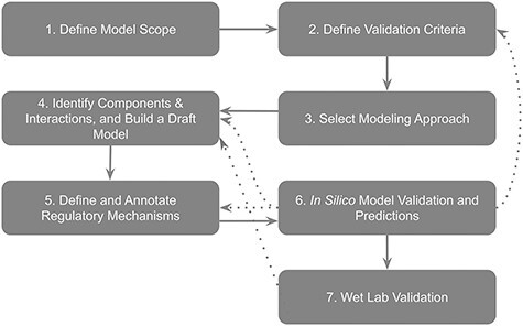
An overview flowchart depicting the process of modeling. Solid arrows indicate the main workflow. Dotted arrows indicate possible needs for the revision of previous steps, as discussed in the main text.

Review of the lac operon regulation system

This protocol is designed to be broadly accessible to biology scientists, established or in-training. As such, no prior training or experience in computational modeling, programming or bioinformatics is needed. Throughout the protocol, we use the widely studied and well-known lac operon system.

As detailed in Figure 2, the lac operon includes a set of three genes: a promoter, a regulator and an operator. The three structural genes are lacZ, encoding β-galactosidase, an enzyme able to metabolize lactose into glucose and galactose, lacY, encoding β-galactoside permease, a transmembrane protein that imports β-galactosides into the cell, and lacA, which encodes the β-galactoside transacetylase, an enzyme responsible for the transfer of an acetyl group from acetyl-CoA to β-galactosides. LacA does not actively participate in lactose metabolism [17, 18].

Figure 2 .

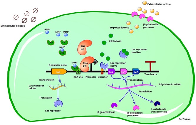
Overview of lac operon regulation. See main text for details about the regulation of the lac operon. The lac operon is under the control of two regulatory molecules, the lac repressor and the CAP. These molecules are responsible for switching the lac operon ON or OFF, depending on sugar availability. In the absence of extracellular glucose (depicted with degradation circles), the hunger molecule cAMP (blue node) binds to CAP (green node) and stabilizes a conformation with a high affinity for the regulator CAP site of DNA (depicted with a green box with a cross). The cAMP-CAP binding favors the binding of the RNA polymerase (orange node) to the promoter (thick black arrow) site. This also happens because, as extracellular lactose (depicted with pale orange nodes) is imported into the cell, a fraction of it is converted to allolactose (green nodes). Allolactose binds to the lac repressor (big purple node), stabilizing a conformation unable to bind the operator (orange box with a black minus). RNA polymerase is thus free to start transcribing the operon. When the operon is active, the three structural genes will be produced, namely lacZ, lacY and lacA. LacI, the gene encoding for the lac repressor, is not part of the operon and is under the control of its own promoter. lacI is continuously transcribed and the repressor protein is always present. The lac repressor binds to the operator, which is partially overlapping with the promoter region. This binding prevents the RNA polymerase from binding and starting the transcription process. Illustration was created with TinkerCell (http://www.tinkercell.com).

The lac operon is controlled by two regulatory molecules: the lac repressor and the catabolite activator protein (CAP). These molecules are responsible for switching the lac operon ON or OFF, depending on sugar availability.

The lac repressor binds to the operator, which is partially overlapping with the promoter region. This binding prevents the RNA polymerase from binding and starting the transcription process. LacI, the gene that encodes the lac repressor, is not part of the operon and is controlled by its own promoter. LacI is continually transcribed, and the repressor protein is always present. As lactose enters a cell, a fraction of it is converted into the inducer allolactose, an isomer of lactose. Allolactose binds to the lac repressor, stabilizing a conformation that is unable to bind the operator. RNA polymerase is thus free to start transcribing the operon. When glucose levels are low, CAP can bind to a site just upstream to the lac operon, the regulator, and facilitates the RNA polymerase attachment to the promoter. The gene that encodes CAP is not part of the lac operon and is constitutively expressed. The binding of CAP to the DNA is regulated by the ‘hunger signal’ molecule, cyclic adenosine monophosphate (cAMP), which is produced in Escherichia coli when glucose levels are low. cAMP binds to CAP and stabilizes a conformation with a high affinity for the regulator [19]. In the absence of binding of the cAMP-CAP complex to the DNA, transcription of the operon is significantly reduced [18, 20, 21]. Thus, the operon is transcribed at a high level only when glucose, the preferred sugar, is absent. E. coli cells presented with a mix of glucose and lactose will induce the lac operon only after the glucose has been depleted [22].

Requirements

Equipment

A computer with a Windows, Mac or Linux operating system, Internet connection and a web browser with WebGL enabled. The hardware specifications of the computer may limit the size of models that can be analyzed within GINsim. We recommend a computer with 4+ GB of RAM and a dual-core processor, in which case use Cell Collective.

Equipment setup

Cell Collective is a web-based application, which does not require installation on one’s computer. Users need to create a (free) account directly in Cell Collective at https://cellcollective.org (under the ‘Research’ panel). Further user support is available via email at support@cellcollective.org.

GINsim can be downloaded from http://ginsim.org.The reader should make sure to download version 2.9 or higher, as older versions do not support the import of SBML-encoded models. They should also ensure that they have Java 1.6 or above installed. Open the downloaded file and follow the installation instructions.

Step 1: Define the scope of the modeled system

The first step of a modeling project is often to decide the scope of the model. Biological networks can be vast, complex and span several scales of biological organization (from molecules to cells, tissues, organisms and even populations). It is critical to understand that computational models are simplifications or abstractions of the real biological system. As such, it is essential to define a model scope that encompasses the minimum number of elements (e.g. pathways) able to address our research question with the data at hand. One can also think of the scope of the modeled system as boundaries defined by the system’s input (e.g., stimuli) and output (e.g., modeled phenomenon and its ‘biomarkers’).

In this protocol, we focus on the lac operon system, one of the first gene regulatory mechanisms to be fully elucidated and characterized [17]. The lac operon is responsible for regulating lactose metabolism in E. coli and other enteric bacteria. Lactose provides the bacterium with an alternative source of carbon when glucose is not present. As such, the scope of the modeled system can be defined by the availability of extracellular glucose and lactose as inputs/stimuli, and lactose metabolism as the model output. As mentioned above, it is important to realize that building a mechanistic computational model is an iterative process, which means that the scope can be adjusted as needed during the entire modeling process.

Step 2: Define validation criteria

One way to assess whether a computational model might be able to answer a given research question, validation criteria should be defined. These criteria will ensure that the constructed model behaves as expected within the model scope defined in Step 1.

Quantitative or qualitative relationships between input(s) and output(s) can constitute validation criteria for computational models. In the case of the lac operon, they can be the relationships between lactose and glucose (inputs) and the lac operon expression (output), because these relationships are well-documented, understood and within the scope of the model. Table 1 presents the four validation criteria, i.e. all possible combinations of the presence and absence of lactose and glucose and the output that the model should produce to be considered useful and correct within this scope.

Table 1.

Validation criteria for the modeled lac operon system

	Glucose	Lactose	lac operon transcription
Validation criterion 1	present	absent	OFF
Validation criterion 2	present	present	OFF
Validation criterion 3	absent	present	ON
Validation criterion 4	absent	absent	OFF

Step 3: Select modeling approach

Once the modeler has decided on the scope and validation criteria, the second step is to select an appropriate modeling technique. Many mathematical and computational frameworks are available to model biological mechanisms and processes. Interested readers should review [23, 24] for detailed summaries of various modeling techniques. Examples include logical models [25], kinetic models (e.g. via ordinary differential equations; ODEs [26]), constraint-based models [27], etc. It is essential to understand that every modeling approach makes different assumptions, and comes with different requisites and constraints and therefore presents different benefits and limitations. Understanding the type of questions that a given computational model can answer is critical, as is the type and amount of data needed to construct and interpret the model. For example, ODE models are very useful to generate quantitative predictions. However, their reliance on kinetic parameters and the required computational complexity and cost limit their usefulness to well-characterized, relatively small, networks/pathways. ODE-based modeling also generally requires a steep learning curve as it relies on complex mathematical equations that describe the system’s kinetics. [24] Constraint-based models are based on the stoichiometry of reactions and are used to calculate optimal flux distributions in metabolic networks [27].

The protocol presented here uses a logical modeling framework. Researchers use this approach to study the dynamics of many biological processes and diseases (e.g. T cell differentiation [2], renovascular disease [28], patient-specific signaling pathways in cancer [29], human immune system [30]), primarily because of its accessible nature. Logical modeling approaches are well suited for qualitative biological problems such as cell fates arising under certain initial conditions or the pathways affected by the perturbation of a particular gene or protein [25, 31, 32]. Like any other approach, logical modeling presents its own limitations. For example, attractors (see Box 1) are computationally expensive to compute due to the exponential growth of the models’ state space. Logical model output is generally discrete, which may be insufficient if one needs to quantify specific concentrations. For a recent and comprehensive review of logical modeling and its broad areas of application, readers should consider [25]. However, the increasing popularity of logical models is also due to, among other reasons, their independence from the scarce availability of kinetic parameters, their scalability and the opportunity they offer for in-depth dynamical analysis while retaining the ability to describe biological processes at the mechanistic level. Moreover, logical models are generally more accessible to a non-modeling audience because their ‘logic-based’ ‘nature closely resembles the language used to describe regulatory mechanisms in wet-lab research publications and the qualitative nature of phenotypic matrices obtained in many genetic screens. The logical rules describing various biological mechanisms are relatively easily applied to construct and ‘read’ the underlying mechanistic computational models [33], lending itself as an intuitive interface between biology and computational modeling. Recent efforts building on these advantages are speeding up the building of large, accurate, and simulatable logical models from comprehensive disease maps [34] and high-throughput data [35].

Box 1:

Introduction to logical modeling

Logical models are composed of components (nodes) connected with directed edges (Figure 3). The individual components of the system can correspond to proteins, complexes, transcription factors, genes or more abstract phenomena such as cellular fates. The directed edges represent causal (direct or indirect) interactions between these components denoting negative influences (e.g. inhibitions, repressions and degradations) or positive ones (e.g. stimulations, activations and synthesis). Logical models can be Boolean or multi-valued. In Boolean models, each component can be either active/expressed/ON (1) or inactive/silent/OFF (0). Multi-valued logical models can assume additional activity values, such as ‘OFF’, ‘medium’ and ‘ON’. The underlying regulatory mechanisms are described by logical expressions that determine the activity level of a component, given the activity states of its direct regulators.

As an example, consider the hypothetical 4-component logical model in Figure 3. Open arrowheads represent positive influences, and bars represent negative ones. In this network, ‘In (input)’ is an external component, able to stimulate the model. In general, components that are not regulated by other components are considered inputs, and their activity is not decided by logical functions. Instead, their activity level(s) can be set before or during a simulation by the user. Conversely, the activity level of each remaining component is determined by their immediate regulators with logical functions reflecting the regulatory mechanisms. For example, the logical function representing the mechanisms regulating Y captures a scenario where Y will be activated at any time point (t + 1) when either X or Z was active at the previous time point (t). Furthermore, components, such as Y, that do not affect the activity level of any other components can be considered outputs (note that model outputs can also be the combination of several components’ activities).

The model’s dynamics depend on the iterative updating of each component’s activity levels. Simulations of logical models can be synchronous (all components are updated at each time point) or asynchronous (components are updated according to a probability or a user-defined priority schema). One can study the dynamics of logical models as they evolve in time, or when the model reaches a steady-state or a set of states (‘attractors’). The purpose of this protocol is to introduce the general workflow of mechanistic modeling and not the intricacies of the logical modeling framework. Readers interested in learning more on the subject (such as the implications of synchronous versus asynchronous updating or state-space analyses) can do so in numerous dedicated publications [36–38].

Figure 3 .

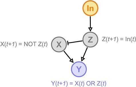
Hypothetical logical model.

Figure 4 .

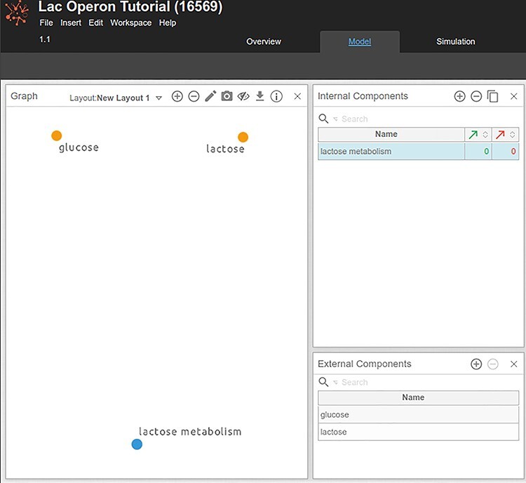
Adding input and output components in Cell Collective. Yellow dots in the ‘Graph’ panel denote external components or inputs, which are components without upstream regulators, and whose activity is controlled by the user. Gray dots correspond to internal components of the model, whose activity is regulated by another model component.

Figure 5 .

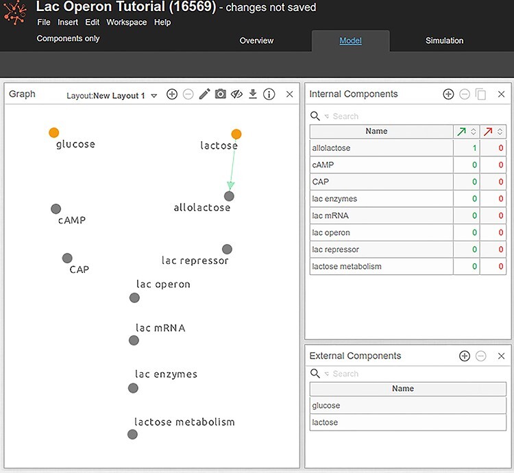
Adding components and their relationships (edges) in a draft model. Orange components correspond to external components, whereas gray components—are non-external/internal components—not visualized in this figure. Selected component is denoted in blue. Note that the reader can move components around the canvas by pressing the Shift key and move the component around, or by switching to the View mode (by clicking on the Pencil icon) and dragging the components where needed.

Introduction to Cell Collective and GINsim

Because of the increasing popularity of logical modeling in biology, many software tools are available to the community. Some commonly used tools include Cell Collective, CellNOpt, GINsim, BoolNet and BooleanNet [25]. In this protocol, we use Cell Collective and GINsim. Cell Collective is a web-based platform that allows users to build and use models without specifying mathematical equations or computer code—addressing one of the major hurdles with computational modeling [39, 40]. As of today, Cell Collective supports logical- and constraint-based [27] modeling approaches. Users can collaboratively construct models, share them directly with others, and simulate and analyze the models in real-time on the web without the need for local software installation and configuration. In addition, Cell Collective provides a database of ~80 curated logical models and nearly 200 genome-scale metabolic models across many biological processes and species. We will introduce Cell Collective in an interactive and just-in-time fashion throughout the protocol. At the moment, the reader should create a free account in Cell Collective at https: //www.cellcollective.org.

We will also use GINsim [41], a logical modeling software that provides a variety of methods for in-depth dynamical analysis of model properties. In addition to Boolean models, GINsim supports models with multi-valued variables. The reader can download and install the latest version from http://ginsim.org. While in this protocol, we will focus on the complementary capabilities of GINsim, a complete tutorial for the tool can be found in [41].

Let’s begin by capturing the scope of the system (defined in the Introduction section) through a model in Cell Collective (Procedure 1).

Procedure 1:

Model scope implementation in Cell Collective.

Sign into Cell Collective (https://cellcollective.org).

Click on ‘New Model’.

Name the model ‘Lac Operon Tutorial’.

Given the scope of the model defined previously, the first components that can be added to the model are the inputs (‘glucose’ and ‘lactose’) and the model output, ‘lactose metabolism. In the ‘Graph’ panel, add these three components by double-clicking anywhere in the panel (Figure 4). Components can be also added by clicking on the ‘plus’ icon in the ‘Internal’ and ‘External Components’ panels.

5) To designate a component as an ‘External Component’ (input), drag the component from the Internal Components panel to the External Components panel (its heading). In our example, ‘glucose’ and ‘lactose’ are inputs to the system and are set as External Components in Cell Collective. ‘lactose metabolism’ is an internal component of the model, regulated by other system components (as we will see later in this protocol).

Step 4: Identify components and their interactions, and build a draft model

Once the modeler has defined the initial scope of the model and identified the preferred modeling approach (and the corresponding tool), the next step is to identify the individual components that will constitute the system and their interactions, and begin constructing a draft of the model. This requires listing the biological entities they want to include in the model and also make a decision on the granularity of representation for each of them. During the first iteration of the modeling process, the knowledge of the researcher can be complemented with static diagrams from published literature, or by accessing public databases. Review articles generally provide lists (and descriptions) of the most important and well-studied components of the reviewed biological processes, which can be used to identify the components that are most relevant to the modeled process. In addition, these reviews often synthesize the discussed components and interactions in diagrams that can be easily depicted and converted into a network diagram, which can further provide the basis of the first draft of the mechanistic model.

Public databases such as KEGG Pathway [42], REACTOME [43], Pathway Commons [44], PANTHER [45], WikiPathways [46], Omnipath [47], BioCyc [48] and Signor [49] constitute an important source of biological knowledge presented in the form of pathways or networks. PathGuide [50] contains information about 670 such resources related to biological pathways and molecular interactions. These are further complemented by commercial tools such as Ingenuity Pathway Analysis or METACORE [51] that also provide curated canonical pathways. Other databases such as Genemania [52], STRING [53], IntAct [54] and BioGRID [55] offer information about individual reported protein–protein interactions (inferred or experimentally validated) that can complement or validate a biological pathway. Many of the aforementioned resources can be easily used to develop the draft mechanistic representation of the system of interest and even provide their data in a standard format that can be directly re-used by modeling software tools. To make this protocol self-contained and allow the reader to follow easily, we have synthesized the required biological knowledge about the lac operon in the Introduction section and in Figure 2.

Figure 6 .

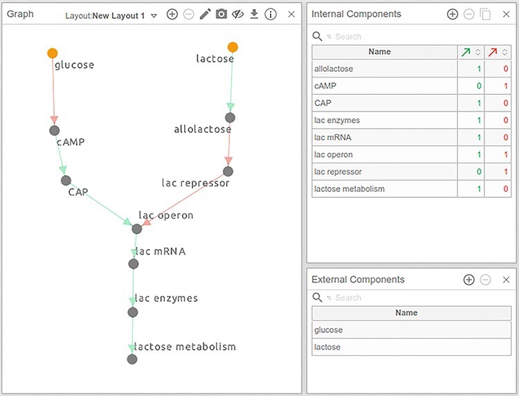
Fully connected network diagram of the lac operon model.

Now that we have defined the scope (Step 1) and the validation criteria (Step 2; Table 1) of the model and have defined the system components and their interactions, we can build a draft model. In Step 3, we already created a model in Cell Collective with three components (‘lactose’, ‘glucose’ and ‘lactose metabolism’) representing the inputs and output of the model. We will now represent the biological knowledge about the lac system (summarized as a network diagram composed of nodes and directed edges Procedure 2). Because Cell Collective automatically translates the diagram into logical rules, the initial network diagram will also become the first draft of a simulatable model that we will further fine-tune in the next section.

Procedure 2:

Building a draft model.

Return to the Lac Operon Tutorial model you started in Cell Collective under Procedure 1.

Under the `Model' tab, by double-clicking in the Graph panel, add four components of the Lac operon system identified in Step 4: cAMP, CAP, allolactose and lac repressor. We assume that the amount of lac repressor is constant and omit LacI and the lac repressor mRNA from the model. Instead, we will focus on capturing the regulatory mechanism of a functional lac repressor. Because of the scope of this model, we also omit the individual lac operon genes; instead, components representing all lac genes and their products are included: lac operon (representing the activity of all three genes lacZ, lacY and lacA), lac mRNA (representing the polycistronic mRNA encoding the three proteins) and lac enzymes (representing β-galactoside permease, β-galactoside and β-galactoside transacetylase).

Add ‘lac operon’, ‘lac mRNA’ and ‘lac enzymes’ components to the model. You should now have 10 components (Figure 5).

From the lac operon overview in the Introduction section, we can also easily derive the directed edges between the components. For example, we know that lactose is converted into allolactose. Add this relationship in Cell Collective by clicking on and dragging an edge from ‘lactose’ to ‘allolactose’ (Figure 5). The hydrolysis of ‘lactose’ into ‘allolactose’ is abstracted in the model as ‘lactose’ activating ‘allolactose’, depicted with a green directed edge.

Next, we know that when allolactose is produced, it binds to the lac repressor, preventing its binding to the lac operator, lifting the repression. This relationship is abstracted in the model as ‘allolactose’ inhibiting lac repressor, depicted with a directed red edge (Figure 6). To draw an inhibitory edge in Cell Collective, create a (positive) edge from ‘allolactose’ to lac repressor and, holding the ‘Shift’ key on your keyboard, click on the edge. The resulting inhibitory edge should be red, as indicated in Figure 6. (For a list of all keyboard shortcuts, hover over the Information ‘i’ icon at the top right of the Graph panel.)

Follow this method to connect all remaining components of the model, resulting in the draft model illustrated in Figure 6.

Step 5: Define and annotate regulatory mechanisms

Cell Collective facilitates biological knowledge- and context-driven creation of logical models and the underlying logic expressions. By design, users can create models without the direct entry of mathematical equations or source code. To define the regulatory mechanism of a component in Cell Collective, they select a component’s activator(s) and/or inhibitor(s) (direct upstream regulators) and create their more complex conditional relationships via the software drag-and-drop user interface.

Simple regulatory mechanisms are automatically generated as part of the ‘model drawing’ feature. For example, when we drew a positive influence between cAMP and CAP in the previous section, we also created the underlying logical expression (‘CAP = cAMP’, which indicates mathematically CAP (t + 1) = cAMP (t)). Similarly, the regulatory mechanism of lac operon has also been automatically depicted as a logical expression (‘lac operon = CAP AND NOT lac repressor’), reflecting the activatory and inhibitory roles of the upstream regulators, CAP and lac repressor, respectively (Figure 7). Note that in logical models, the simultaneous influences of an activator and an inhibitor on a component (such as lac operon in the presented model) are expressed by an AND operator to indicate the ‘opposing influences’ of each component. In a more complex case, for example, where multiple activators and inhibitors are present, the negative regulators can be defined selectively to work ‘against’ specific positive regulators. In Cell Collective, these selections can be made under the ‘Dominance’ option in the Regulatory Mechanism panel (Figure 7).

Figure 7 .

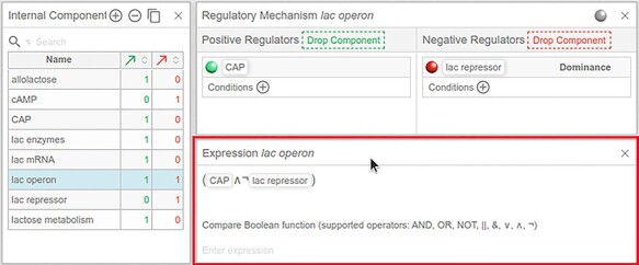
Generation of Boolean expressions. The panel boxed in red shows the Boolean function associated with each component, created when developing the model in the ‘Graph’ panel (not shown here) or the ‘Regulatory Mechanism’ panel. Note that the ‘Expression’ panel is not part of the model workspace by default, but users can add it by clicking on Insert - > Panel - > Model - > Regulation Expression at the top of the page (under the model name).

Additional, more complex regulatory mechanisms involving, for instance, conditional relationships among multiple upstream regulators, can be easily defined in the ‘Regulatory Mechanism’ panel (Figure 8). An example would be the requirement of a co-factor for a transcription factor to initiate the transcription of a gene. Cell Collective represents such relationships as ‘conditions’. As illustrated in Figure 8, the ‘transcription factor’ would be defined as an activator of the gene, and only activate gene if co-factor is active. Note that even more complex conditional relationships can be defined, with multiple conditions, as well as conditions of conditions (sub-conditions), depending on the complexity of the underlying regulatory mechanism [33].

Figure 8 .

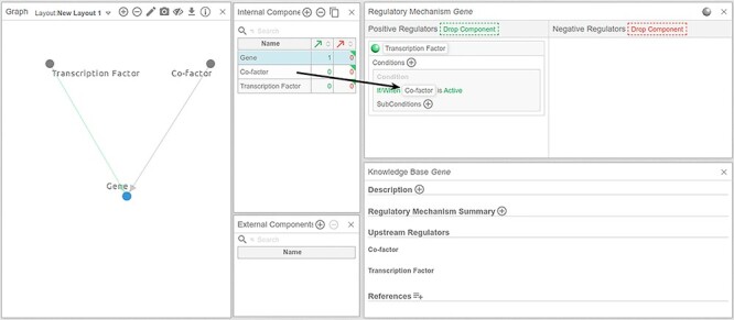
Drag-and-drop components to build the regulatory mechanism of a given component. To define the regulatory mechanism of a given component, drag components from the ‘Internal/External Components’ panels to the corresponding areas in the ‘Regulatory Mechanism’ panel.

A critical, and often overlooked, part of developing computational models is annotation. Well annotated models facilitate transparency and reusability [56, 57]. Cell Collective allows the annotation of components at multiple levels, including the model, the regulatory mechanism of a component, and individual interactions. Model-level annotations contain general model information, such as its scope and the validation criteria, to help the community understand if and how it may be used as a starting point for their research questions. Users can add model annotations in the ‘Description’ tab. They can add more detailed annotations at the level of each component’s regulatory mechanism and interactions during the model-building process in the ‘Knowledge Base’ (KB) panel (Figure 9). In the KB panel, users can describe the meaning of each component of the model while providing unique identifiers when available. For instance, they can describe individual interactions (e.g. the activation of CAP by cAMP) at the level of biochemical and mechanistic regulation, while providing published evidence to support the mechanism.

Figure 9 .

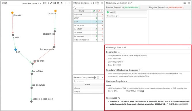
Annotations of components and interactions in Cell Collective. The KB panel (boxed in red) enables users to provide detailed information about each model component and its immediate regulating interactions. Each piece of text, or evidence, is citable with a PMID or DOI, allowing to connect each piece of support to its underlying sources. Furthermore, by right-clicking on the citation or reference, the user can specify if the source is primary or non-primary (e.g. a review article) source, and whether the support (data) in the source comes from human or animal experiments.

Figure 10 .

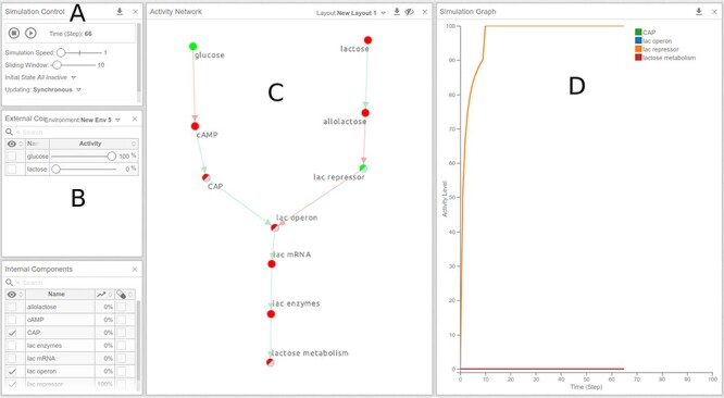
Real-time simulation of the lac operon model under a high-glucose, no lactose environment. The activity levels of all components of the model are illustrated in the ‘Activity Network’ panel (C) with colors of the component ranging from red (0) to green (100) and in the ‘Simulation Graph’ panel (D) as a time-series graph, which shows the activity levels of selected components over time. Note that the time scale is arbitrary, measured in time steps. Components to be viewed in the ‘Simulation Graph’ panel can be added by clicking on the components in the network or by checking the first column in the ‘Internal/External Components’ tables.

Step 6: In silico model validation and predictions

Once all the regulatory mechanisms and corresponding logical expressions for each component of the model are defined, we can simulate the model to test whether it can reproduce the dynamics and behaviors defined in the validation criteria. As the rules are assigned locally, there is no guarantee that the global behavior will comply with those criteria or the descriptions in the published literature. Users should expect several revisions of regulatory mechanisms, rules, re-wiring and, possibly, additions or deletions of components and edges while fine-tuning the model.

Cell Collective offers several simulation tools to interrogate and visualize the dynamics of a model interactively and in real-time. Although models in Cell Collective are Boolean as discussed in the Step 3, inputs and outputs are semi-quantitative during the simulations, to describe the relative activity of a particular model component in response to environmental signals or perturbations in the model [1, 2, 58]. Users can define the activity levels of external components (inputs) on a scale from 0 to 100, representing the percent chance of the external component to be active or inactive at any time during the simulation. The overall activity of any internal component or output of the model spans the same scale, representing the average activity (fraction of ones) over a defined number of previous time steps. For example, if a component has an activity level of 50%, it means that the component assumed the same number of active and inactive states over the last n number of iterations, likened to the concept of ‘moving average’. The number of iterations is defined with the ‘Sliding Window’ parameter in the real-time simulation feature (Procedure 3) [39]. While the values of inputs (e.g. glucose set to 90%) do not directly correspond to a specific, measurable biological property (such as concentration), users can interpret the activity levels semi-quantitatively [39, 59]. For example, they can represent ‘high amounts of glucose in the environment’ by setting glucose activity to 80–100% and ‘low amounts of environmental glucose’ by setting it to 0–10%. Cell Collective can simulate dose–response experiments and show how components’ dynamics evolve when the activity of inputs increases.

In the Procedure 3 box, we illustrate how to simulate the four validation criteria (Table 1) to assess the usefulness of the model using Cell Collective’s real-time and dose–response simulation tools.

Figure 11 .

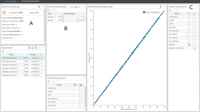
Dose–response curve analysis of lactose metabolism under lactose varying conditions. Glucose is absent from the environment. Instead of selecting a single activity level of the input, users can select a range of activities by adding new Environments under the ‘External Components’ panel (B). Here, Glucose is set to 0, and Lactose varies from 0 to 100. Make sure that the appropriate environment is selected in the ‘Experiment Settings’ panel (A). The components represented on the y- and x-axes can be selected by checking appropriate boxes in the ‘Graph Components’ panel (C).

Figure 12 .

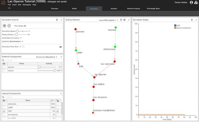
Real-time simulation of effects of CAP knock-out mutation.

Procedure 3:

Model validation.

Criterion 1: Lactose metabolism should be inactive when glucose is present and lactose is absent from the environment.

Access the real-time simulation workspace under the ‘Simulation’ tab in your model in Cell Collective.

Ensure Simulation Control Settings (Figure 10A) are configured to.

Simulation Speed = 1.

Sliding Window = 10.

Define the Environment of the model in the External Components panel (Figure 10B) by adding glucose:

Adjust the ‘glucose’ slider to 100, which will simulate the availability of glucose during each step of the simulation.

Ensure that the ‘lactose’ slider is set to 0, which will simulate complete absence of lactose from the environment.

To view ‘lactose metabolism’ as the measured variable (output) of the model click on the component in the Activity Network panel (Figure 10C). This will add ‘lactose metabolism’ to the Simulation Graph panel (Figure 10D). We can also observe the dynamics of other components of the model, by clicking, for example, on lac operon, CAP and lac repressor.

Start the simulation by clicking on the play (▶) button under the Simulation Control panel.

Click the pause (||) button after ~75 steps (shown on the x-axis).

The activity of each component can be observed in the Simulation Graph panel as it evolves in time. To see specific components in the graph, hover the cursor over the component name in the legend. Furthermore, the Activity Network panel shows the activity levels of all components in the network as colored nodes, where bright green corresponds to complete (100%) activation and red corresponds to a complete absence of activation (0%). Shades of these colors correspond to activity levels between 0 and 100.

Simulation result—Under this environmental condition (where glucose is present and lactose is absent), you should observe that ‘lactose metabolism’ is inactive, as expected (Figure 10D).

Validation Criteria 2–4.

Continue to simulate the model (press (▶) button) under the remaining three environmental conditions, by moving the glucose and lactose sliders between 0 and 100. You can also set the sliders to intermediate values to observe partial activation responses within the system.

The response of a model output or various components can be simulated in Cell Collective using the Dose Response tool under the ‘Analysis’ tab as illustrated in Figure 11.

Figure 13 .

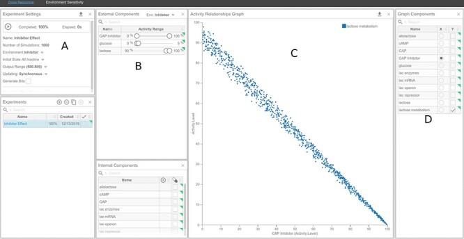
Dose–response curve of CAPInhibitor and its effect on lactose metabolism under high-lactose and low-glucose environments. (A) Experiment Settings panel. (B) External Components panel. (C) Activity Relationships panel. (D) Graph Components panel.

Figure 14 .

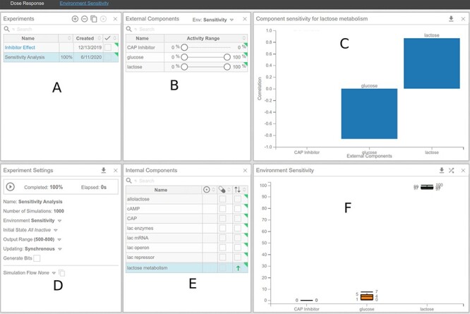
Environment sensitivity analysis.

Figure 15 .

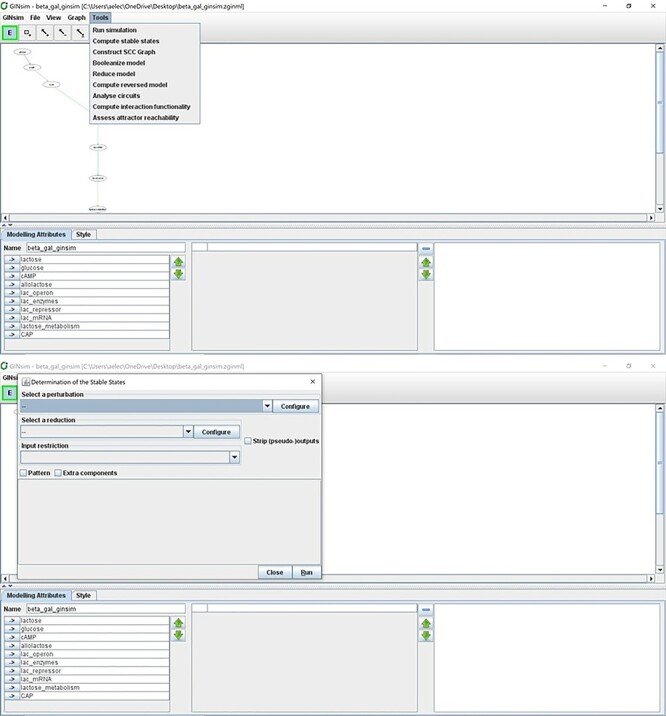
Computing stable states of the model using GINsim.

Figure 16 .

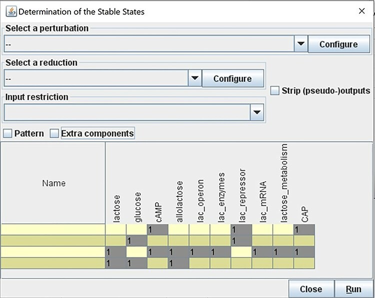
Calculating all possible stable states for the lac operon model, computed with the software GINsim. Value 1 represents the ON state (also corresponding to 100% activity level in Cell Collective).

Predicting the effect of mutations and modulators

When we are satisfied with the model structure and its ability to reproduce the defined validation criteria, we can use it for performing additional in silico experiments to develop new hypotheses or refine existing ones. For example, one can simulate perturbations of the system by constitutively inactivating components, thus generating in silico knock-outs, simulate inhibitions or overexpressions and make specific predictions before testing them at the bench. One of the advantages of computational models is the possibility to easily simulate the systematic effects of individual or combinatorial perturbations of many components of the model. Examples are reviewed in [2, 58, 60–63].

We can test different scenarios on the lac operon model, such as the effects of mutations on the system’s dynamics. For instance, Procedure 4 shows simulations of the effects of CAP loss-of-function on lactose metabolism under environmental conditions conducive to lac operon expression.

Procedure 4:

Simulating the effects of CAP loss of function on lactose metabolism.

In Cell Collective, mutations (knock-out and overexpression) can be introduced by checking the box next to a component of interest in the ‘Internal Components’ panel within the ‘Simulation’ workspace (Figure 12).

Check the box next to CAP such that the check-mark is red, indicating a knock-out mutation. Clicking on the box twice will add a green check-mark, indicating an overexpression and clicking on the box for the third time will un-check the box, returning the corresponding component to its wild-type status.

Set the environmental condition that is conducive to lac operon expression by setting extracellular glucose and lactose to appropriate levels of 0 and 100, respectively.

Select the components whose activity you would like to observe in the ‘Simulation Graph’ panel by clicking on them in the network diagram. Because we are interested in observing the effects of ‘CAP’ loss-of-function on lactose metabolism, select the ‘CAP’ and ‘lactose metabolism’ components.

Start the simulation. After ~50–60 steps, we can observe that, while ‘allolactose’ and ‘cAMP’ reach 100%, ‘CAP’, lac enzymes, lac mRNA, lac operon, lac repressor and ‘lactose metabolism are entirely inactive. The simulation recapitulates the dynamic behavior of the system in a scenario where the hunger signal, cAMP, is active due to the absence of ‘glucose’, and ‘allolactose’ is active because of the presence of extracellular ‘lactose’. ‘Allolactose’ subsequently binds and activates the lac repressor. However, the ‘CAP’ loss-of-function mutation precludes the binding of ‘CAP’ to the DNA and the subsequent recruitment of the RNA polymerase. The lac operon thus remains inactive, no lac enzymes are translated and no lactose metabolism takes place.

While the previous example illustrated the simulation of complete knock-out/loss-of-function mutations, partial mutations, such as knock-down/down-regulation or overexpression, can also be simulated. We do so by adding an external component that will inhibit or activate the component whose expression we want to perturb. Users can subsequently set the activity of the newly introduced external component to the desired value. Procedure 5 illustrates this concept.

Procedure 5:

Partial in silico mutations.

Add a new external component, CAP Inhibitor, to the Lac operon model.

Add an inhibitory edge from ‘CAP Inhibitor’ to ‘CAP’.

To simulate the effect of partial inhibition of ‘CAP’ using the real-time simulation tool, change the activity levels of ‘CAP Inhibitor’ and select ‘CAP’, ‘CAP Inhibitor’ and ‘lactose metabolism’ as variables to observe during the simulation. Start the simulation (not pictured).

Dose response (Figure 13): To simulate a dose–response of lactose metabolism to ‘CAP Inhibitor’, go to the dose response analysis tool, under the ‘Analysis’ tab.

In the ‘Experiment Settings’ add a new experiment.

In the ‘External Components’ panel (B), set ‘glucose’ to range from 0 to 5%, ‘CAP Inhibitor’ to range from 0 to 100% and lactose to range from 90 to 100%. Notice that a new environment, called ‘New Env 1’, is created, accessible in the header of the ‘External Components’ panel. Rename it to ‘Inhibitor’ by clicking on the name.

Under the ‘Experiments Settings’ panel (A), change the Environment from ‘Default’ to the one created in the previous step, ‘Inhibitor’.

In the ‘Graph Components’ panel (D), select ‘CAP Inhibitor’ for the x-axis and ‘lactose metabolism’ for the y-axis.

Start the experiment in the ‘Experiment Settings’ panel (A).

The dose–response will be plotted in the ‘Activity Relationships Graph’ panel (C).

Reachability and control of biological systems

So far, we have presented procedures where users set initial conditions and observe the—a priori unknown—results of simulations. However, computational models also lend themselves to study where one wants to know which conditions must be met for the model to reach a known result, such as ‘under what extracellular conditions is the activity of component X maximal?’ To illustrate this type of analysis with our model, we will try to answer the following question ‘Under what levels of lactose and glucose can we get the highest levels of lactose metabolism?’

To address such questions pertaining to the sensitivity of a system towards the environment in Cell Collective, we use the ‘Environment Sensitivity’ workspace in the ‘Analysis’ tab. Follow the instructions illustrated in Procedure 6 to conduct the environment sensitivity analysis.

Procedure 6:

Reachability and environment sensitivity analysis.

In the lac operon model in Cell Collective, access the Environment Sensitivity workspace via the Analysis tab (Figure 14).

In the ‘Experiments’ panel (Figure 14A), add a new experiment, named ‘Sensitivity Analysis’.

To consider all possible environmental input combinations, create a new environment in the ‘External Components’ panel (Figure 14B), where ‘glucose’ and ‘lactose’ vary from 0 to 100, while setting ‘CAP Inhibitor’ to 0. Name the environment ‘Sensitivity’. To limit the possible environments, choose alternative ranges to suit your needs.

In the ‘Internal Components’ panel (Figure 14E), select ‘lactose metabolism’ and change the ‘Optimize’ column (two vertical opposite arrows) to a green, upward arrow, to tell the software we want to maximize the activity level of ‘lactose metabolism’ under the selected range of environmental inputs.

In the ‘Experiments Settings’ panel (Figure 14D), change the Environment to ‘Sensitivity’. Change the number of Simulations to 1000.

Start the experiment in the ‘Experiment Settings’ panel.

The ‘Environment Sensitivity’ panel (Figure 14F) will generate an environmental condition in the context of activity levels of ‘lactose’ and ‘glucose’ that will result in high levels of ‘lactose metabolism’. The ‘Component Sensitivity’ panel (Figure 14C) shows the effect size that each input has on ‘lactose metabolism’. In particular, the results show that ‘glucose’ has an overall negative effect on ‘lactose metabolism’, while ‘lactose’ has a positive effect on ‘lactose metabolism’. Results from this analysis are consistent with the simulations and analyses conducted in the previous sections: ‘lactose metabolism’ will be the most active under high lactose and low/no glucose conditions.

State-space and attractors

Another layer of analyses of computational models includes the exploration of the entire space of states that a model can find itself in as a result of its environmental stimuli or various perturbations. Because each component of a Boolean network can take the values 0 or 1, the entire model can exist in at most 2ⁿ different states. Using either synchronous or asynchronous updates (see Box 1) and fixed inputs (e.g. ‘lactose’ and ‘glucose’ set to 0 or 1 for the entirety of the simulation), the dynamics of a logical model will eventually lead to a set of states from which it cannot leave, called an ‘attractor’. Attractors can be either stable states (states from where our system cannot escape without external intervention), representing, for example, cell fates (apoptosis, cell differentiation, or in our case active or inactive ‘lactose metabolism’) or more complex attractors, for instance, representing oscillatory behaviors [36]. An attractor can be considered as representing a stable and long-term behavior of the modeled system. In this section, we will use the GINsim software tool to illustrate the analysis of state-space and attractors for the lac operon [41]. Follow Procedure 7 to import the Cell Collective lac operon model and perform steady-state analysis in GINsim.

Procedure 7:

Importing the model in GINsim and performing steady-state analysis.

Export the Lac operon model from Cell Collective in the SBML-qual format [53, 54]. Under your Lac operon model in Cell Collective, click on File - > Download - > SBML.

Open GINsim and from the Start menu select New Model. Then, click on File - > Import. Select SBML-qual from the Import options.

Select ‘Show it’ in the subsequent preprocessing panel.

Rename the model to ‘beta_gal_ginsim’ in the Name textbox.

You can adjust the network model layout by moving the individual components or by selecting built-in layouts from the menu (View).

Select Tools - > Compute Stable States (Figure 15).

A second panel will open where the user can choose optional model reduction or specify perturbations. Press Run to compute all possible steady states of the model.

A table with a summary of the steady states of the model will be displayed once the computation finishes (Figure 16). Results show that the lac operon is ON when lac repressor is absent, lactose is present and glucose is absent. These results align with the validation criteria (Table 1) and with the Cell Collective simulation results discussed earlier.

Adding nodes or reactions to a model can change the reachable states. Figure 17 shows the stable states computed when we add ‘CAP inhibitor’.

Figure 17 .

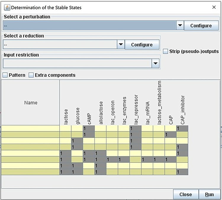
Adding nodes to the model will result in different dynamics and different set of stable states. The addition of the CAP inhibitor resulted in four more stable states of the model. The lac operon will be ON only in the absence of CAPs inhibitor, and when glucose is absent.

Procedure 8:

Adding nodes to the model in GINsim.

In GINsim, select to add a new component to the model.

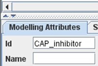
Then, add the name of the component to the Id box in the bottom left panel:

Select to add the inhibition from CAP inhibitor to CAP.

Proceed as explained in Procedure 7 to compute stable states.

The addition of the ‘CAP inhibitor’ resulted in four more stable states of the model. We see that the lac operon is ON only in the absence of ‘CAP inhibitor’, and when ‘glucose’ is absent, which corresponds to our biological knowledge about the CAP mechanism of action.

Step 7: Wet-lab validation

The observations resulting from the procedures illustrated above might generate new hypotheses regarding the modeled system, which can be validated experimentally. A validated prediction means that using the model generated a reliable hypothesis, potentially saving time and valuable resources. An invalidated prediction can still stimulate further investigations of the modeled system by, for example, revisiting the model to identify gaps in its structure, its parametrization or the simulation and analysis procedures.

The scope of the model, for example the level of abstraction (e.g. cellular or molecular), modeling approach and the type of data generated from the model will provide a starting point on how the model predictions can be further validated using wet-lab experimentation. In the case of logical models, Cell Collective has been used to investigate the qualitative impact of perturbations on the activity of various parts of the network. For example a logical model of signal transduction in T cells was used to predict the role and impact of the knock-out and overexpression of Caveolin-1 (an important scaffold protein) on T cell signaling [60]. The output of Cell Collective—differential activity levels of all model components under normal and perturbed conditions—was subsequently validated in an in vivo mouse model using differential gene expression analysis and qualitative immunochemistry—output of which can be intuitively connected with the logical model predictions. Another recent study highlights the potential of mechanistic modeling in precision medicine [29]. In particular, ex vivo high-throughput screening of pancreatic cancer samples was used to generate patient-specific logical models. In this study, the model output (similar to Cell Collective output) was continuous, enabling the measure of perturbation effect on the activity level of other network components. These models were, in turn, used to predict the effect of 174 combinatorial perturbations on cancer-specific pathways, measured as activity level of the pathway components. The authors subsequently validated three most highly ranked predicted combinatorial perturbations on cancer cell lines and mouse models. As introduced in the previous section, logical models can be analyzed to identify attractors—stable sets of states—that can, for example, represent and correspond to cell phenotype. An intuitive example of such utility is the study of cell differentiation. In particular, the binary activity of transcription factors in a given attractor can be associated with the realization of a specific cell fate. For example, authors analyzed with GINsim, the state space of a logical model of signal transduction network governing the differentiation of CD4+ T cells into effector T cells, and identified attractors with new patterns of transcription factor activity, effectively predicting novel T cell phenotypes [64]. Such phenotypes can be further validated with well-established T cell differentiation assays and molecular techniques used to identify T cell (sub-)populations involving, for example, the detection of expression of specific transcription factors [65].

Timing and anticipated results

Following the entire protocol, as described above, takes ~3 h. Applying the protocol to model other biological processes will of course change this timing, depending on the size and complexity of the system to model, the availability (and comprehensiveness) of resources with synthetic knowledge about the system’s components (review articles, pathway databases, etc.).

This protocol will result in a mechanistic (logical) model of the lac operon regulatory system that can serve as a starting point for the reader to expand the model further and, using the newly acquired knowledge, to build models of other biological systems. A version of the model described in the protocol, encoded in the SBML-qual format [66, 67], is provided as Supplementary File 1. The reader can use it as the ‘answer key’ in case their modeling outputs do not match the outputs presented in the protocol.

Conclusions

Herein, we describe a generalized step-by-step approach to abstracting, representing and simulating a biological system in the form of a mechanistic computational model. We contextualized the protocol within a well-characterized gene regulatory system—the lac operon. The protocol can be applied to other biological systems and processes. The protocol also introduces Cell Collective, a web-based modeling platform with a user-friendly interface (without the need to write complex mathematical equations or computer code) for constructing, annotating and simulating/analyzing the model. One of the important advantages is that the user can perform real-time analyses and simulations testing different hypotheses. We also illustrated how the constructed model can be used to recapitulate the known dynamics of the system and study the effect of mutations on the lac operon system. In the last part of the protocol, we used the software GINsim to complete the analysis by calculating the stable states of the model. We hope that this protocol will make computational systems modeling more approachable while allowing readers to identify and utilize fundamental modeling aspects that they can immediately begin utilizing in his/her system of interest.

More complex model representation of the lac operon system

At the beginning of this practical guide, we discussed the importance of selecting and understanding the model’s scope. For this guide’s purpose, we decided that the model would include glucose and lactose regulating lactose metabolism through relatively simple pathways. A computational model of a broader scope would be needed to explore more complex aspects of the lac operon system. For example, one could model inducer exclusion—a phenomenon whereby glucose can inhibit the transport of extracellular lactose by the lac permease (in addition to catabolite repression) [20, 21].

In addition, the lac operon can exhibit bi-stability, in the sense that it can exist in two states: induced and uninduced [68–73]. A system is called bi-stable if it can rest in two distinct stable states, e.g. operon induced and operon not induced. Some bi-stable systems can also present switch-like behavior, enabling them to alternate between the two stable states. For example, when external lactose is transported into the cell, it is converted into allolactose. Allolactose subsequently induces the operon, causing the synthesis of more permease molecules that can transport more external lactose, which is then converted into more allolactose. Several studies have been published concerning the bi-stability of the lac operon, and several models have been developed addressing this issue. Examples of models of the lac operon system with a larger scope focus on diauxic growth [20], feedback regulation [72], bi-stability as well as the effects of catabolite repression and inducer exclusion in the lac operon [68], or a more detailed Boolean model by Veliz-Cuba and Stigler [71], also available in Cell Collective (ModeID 5128; https://research.cellcollective.org/?dashboard=true#5128:1/lac-operon/1).

Key Points

• The described guide will help researchers begin incorporating mechanistic computational modeling into their research inquiries.

• Readers will be able to define the scope and validation criteria of the desired model.

• Non-experts will be able to quickly begin building, simulating and (computationally) validating their models.

• We hope this guide will make mechanistic computational modeling more accessible to a broad range of scientists and teachers.

Anna Niarakis is an Associate Professor at UEVE, Saclay. Her research focuses on the application of computational systems biology approaches in human diseases, including the construction of disease maps, tool development for model inference, network integration and dynamical modeling.

Tomáš Helikar is an Associate Professor in the Department of Biochemistry at the University of Nebraska-Lincoln. His research focuses on the use of integrative multi-approach modeling pipelines for dynamical analysis of biological networks. More precisely, his studies focus on understanding how aberrant changes in biological networks result in disease so that we could strategically develop more effective therapies.

Funding

National Institutes of Health (grant no. 1R35GM119770–04) to T.H.

References

- 1. Helikar T, Konvalina J, Heidel J, et al. Emergent decision-making in biological signal transduction networks. Proc Natl Acad Sci U S A 2008;105:1913–8. [DOI] [PMC free article] [PubMed] [Google Scholar]
- 2. Puniya BL, Todd RG, Mohammed A, et al. A mechanistic computational model reveals that plasticity of CD4+ T cell differentiation is a function of cytokine composition and dosage. Front Physiol 2018;9:878. [DOI] [PMC free article] [PubMed] [Google Scholar]
- 3. Kahlem P, Birney E. Dry work in a wet world: computation in systems biology. Mol Syst Biol 2006;2:40. [DOI] [PMC free article] [PubMed] [Google Scholar]
- 4. Fisher J, Henzinger TA. Executable cell biology. Nat Biotechnol 2007;25:1239–49. [DOI] [PubMed] [Google Scholar]
- 5. Chylek LA, Harris LA, Faeder JR, et al. Modeling for (physical) biologists: an introduction to the rule-based approach. Phys Biol 2015;12:045007. [DOI] [PMC free article] [PubMed] [Google Scholar]
- 6. Meier-Schellersheim M, Fraser IDC, Klauschen F. Multiscale modeling for biologists. Wiley Interdiscip Rev Syst Biol Med 2009;1:4–14. [DOI] [PMC free article] [PubMed] [Google Scholar]
- 7. Schultze JL. Teaching ‘big data’ analysis to young immunologists. Nat Immunol 2015;16:902–5. [DOI] [PubMed] [Google Scholar]
- 8. Faeder JR. Toward a comprehensive language for biological systems. BMC Biol 2011;9(68). [DOI] [PMC free article] [PubMed] [Google Scholar]
- 9. Afgan E, Baker D, Batut B, et al. The galaxy platform for accessible, reproducible and collaborative biomedical analyses: 2018 update. Nucleic Acids Res 2018;46:W537–44. [DOI] [PMC free article] [PubMed] [Google Scholar]
- 10. Cvijovic M, Höfer T, Aćimović J, et al. Strategies for structuring interdisciplinary education in systems biology: an European perspective. NPJ Syst. Biol. Appl Ther 2016;2:16011. [DOI] [PMC free article] [PubMed] [Google Scholar]
- 11. Woodin T, Carter VC, Fletcher L. Vision and change in biology undergraduate education, a call for action—initial responses. CBE—Life Sci Educ 2010;9:71–3. [DOI] [PMC free article] [PubMed] [Google Scholar]
- 12. National Research Council. Next Generation Science Standards: For States, By States. Washington, DC: The National Academies Press. 2013. 10.17226/18290. [DOI]
- 13. Crowther A, Bergan-Roller HE, Galt NJ, et al. Discovering prokaryotic gene regulation with simulations of the trp operon. CourseSource 2018;5. [Google Scholar]
- 14. Crowther A, Bergan-Roller HE, Galt NJ, et al. Discovering prokaryotic gene regulation by building and investigating a computational model of the lac operon. CourseSource 2019;6. [Google Scholar]
- 15. Bergan-Roller HE, Galt NJ, Dauer JT, et al. Discovering cellular respiration with computational modeling and simulations. CourseSource 2017;4. [Google Scholar]
- 16. Helikar T, Cutucache CE, Dahlquist LM, et al. Integrating interactive computational modeling in biology curricula. PLoS Comput Biol 2015;11:e1004131. [DOI] [PMC free article] [PubMed] [Google Scholar]
- 17. Jacob F, Monod J. Genetic regulatory mechanisms in the synthesis of proteins. J Mol Biol 1961;3:318–56. [DOI] [PubMed] [Google Scholar]
- 18.Griffiths AJF, (ed). Modern Genetic Analysis. New York: W.H. Freeman, 1999.
- 19. Saier MH, Chauvaux S, Cook GM, et al. Catabolite repression and inducer control in gram-positive bacteria. Microbiology 1996;142:217–30. [DOI] [PubMed] [Google Scholar]
- 20. Wong P, Gladney S, Keasling JD. Mathematical model of the lac operon: inducer exclusion, catabolite repression, and diauxic growth on glucose and lactose. Biotechnol Prog 1997;13:132–43. [DOI] [PubMed] [Google Scholar]
- 21.Griffiths AJ, Miller JH, Suzuki DT, Lewontin RC, Gelbart, (eds). An Introduction to Genetic Analysis, 7th edn. New York: W.H. Freeman, 2000.
- 22. Siegal ML. Shifting sugars and shifting paradigms. PLoS Biol 2015;13:e1002068. [DOI] [PMC free article] [PubMed] [Google Scholar]
- 23. Keurentjes JJB, Molenaar J, Zwaan BJ. Predictive modelling of complex agronomic and biological systems. Plant Cell Environ 2013;36:1700–10. [DOI] [PubMed] [Google Scholar]
- 24. Le Novère N. Quantitative and logic modelling of molecular and gene networks. Nat Rev Genet 2015;16:146–58. [DOI] [PMC free article] [PubMed] [Google Scholar]
- 25. Abou-Jaoudé W, Traynard P, Monteiro PT, et al. Logical modeling and dynamical analysis of cellular networks. Front Genet 2016;7:94. [DOI] [PMC free article] [PubMed] [Google Scholar]
- 26. Bergmann FT, Hoops S, Klahn B, et al. COPASI and its applications in biotechnology. J Biotechnol 2017;261:215–20. [DOI] [PMC free article] [PubMed] [Google Scholar]
- 27. Orth JD, Thiele I, Palsson BØ. What is flux balance analysis? Nat Biotechnol 2010;28:245–8. [DOI] [PMC free article] [PubMed] [Google Scholar]
- 28. Williams E, Chade AR. A Boolean model of microvascular rarefaction to predict treatment outcomes in renal disease. Sci Rep 2020;10:440. [DOI] [PMC free article] [PubMed] [Google Scholar]
- 29. Eduati F, Jaaks P, Wappler J, et al. Patient-specific logic models of signaling pathways from screenings on cancer biopsies to prioritize personalized combination therapies. Mol Syst Biol 2020;16:e8664. [DOI] [PMC free article] [PubMed] [Google Scholar]
- 30. Puniya BL, Mohammed A, Amin R, et al. A comprehensive mechanistic model of the human immune system to study immuno-dynamics. Forthcoming. bioRxiv. doi: https://10.1101/2020.03.11.988238.
- 31. Wynn ML, Consul N, Merajver SD, et al. Logic-based models in systems biology: a predictive and parameter-free network analysis method. Integr Biol 2012;4:1323. [DOI] [PMC free article] [PubMed] [Google Scholar]
- 32. Helikar T, Kochi N, john k, et al. Boolean modeling of biochemical networks. Open Bioinforma J 2011;5:16–25. [Google Scholar]
- 33. Helikar T, Kowal B, Madrahimov A, et al. Bio-logic builder: a non-technical tool for building dynamical, qualitative models. PLoS One 2012;7:e46417. [DOI] [PMC free article] [PubMed] [Google Scholar]
- 34. Aghamiri SS, Singh V, Naldi A, et al. Automated inference of Boolean models from molecular interaction maps using CaSQ. Bioinformatics 2020;btaa484. [DOI] [PMC free article] [PubMed] [Google Scholar]
- 35. Gjerga E, Trairatphisan P, Gabor A, et al. Converting networks to predictive logic models from perturbation signalling data with CellNOpt. bioRxiv 2020; 2020.03.04.976852. [DOI] [PMC free article] [PubMed] [Google Scholar]
- 36. Schwab JD, Kühlwein SD, Ikonomi N, et al. Concepts in Boolean network modeling: what do they all mean? Comput Struct Biotechnol J 2020;18:571–82. [DOI] [PMC free article] [PubMed] [Google Scholar]
- 37. Albert R, Thakar J. Boolean modeling: a logic-based dynamic approach for understanding signaling and regulatory networks and for making useful predictions. Wiley Interdiscip Rev Syst Biol Med 2014;6:353–69. [DOI] [PubMed] [Google Scholar]
- 38. Wang R-S, Saadatpour A, Albert R. Boolean modeling in systems biology: an overview of methodology and applications. Phys Biol 2012;9:055001. [DOI] [PubMed] [Google Scholar]
- 39. Helikar T, Kowal B, McClenathan S, et al. The cell collective: toward an open and collaborative approach to systems biology. BMC Syst Biol 2012;6:96. [DOI] [PMC free article] [PubMed] [Google Scholar]
- 40. Helikar T, Kowal B, Rogers JA. A cell simulator platform: the cell collective. Clin Pharmacol Ther 2013;93:393–5. [DOI] [PMC free article] [PubMed] [Google Scholar]
- 41. Naldi A, Hernandez C, Abou-Jaoudé W, et al. Logical modeling and analysis of cellular regulatory networks with GINsim 3.0. Front Physiol 2018;9:646. [DOI] [PMC free article] [PubMed] [Google Scholar]
- 42. Kanehisa M, Goto SKEGG. Kyoto encyclopedia of genes and genomes. Nucleic Acids Res 2000;28:27–30. [DOI] [PMC free article] [PubMed] [Google Scholar]
- 43. Fabregat A, Jupe S, Matthews L, et al. The reactome pathway knowledgebase. Nucleic Acids Res 2018;46:D649–55. [DOI] [PMC free article] [PubMed] [Google Scholar]
- 44. Cerami EG, Gross BE, Demir E, et al. Pathway commons, a web resource for biological pathway data. Nucleic Acids Res 2011;39:D685–90. [DOI] [PMC free article] [PubMed] [Google Scholar]
- 45. Thomas PD, Campbell MJ, Kejariwal A, et al. PANTHER: a library of protein families and subfamilies indexed by function. Genome Res 2003;13:2129–41. [DOI] [PMC free article] [PubMed] [Google Scholar]
- 46. Kutmon M, Riutta A, Nunes N, et al. WikiPathways: capturing the full diversity of pathway knowledge. Nucleic Acids Res 2016;44:D488–94. [DOI] [PMC free article] [PubMed] [Google Scholar]
- 47. Ceccarelli F, Turei D, Gabor A, et al. Bringing data from curated pathway resources to Cytoscape with OmniPath. Bioinformatics 2020;36:2632–33. [DOI] [PubMed] [Google Scholar]
- 48. Caspi R, Altman T, Billington R, et al. The MetaCyc database of metabolic pathways and enzymes and the BioCyc collection of pathway/genome databases. Nucleic Acids Res 2014;42:D459–71. [DOI] [PMC free article] [PubMed] [Google Scholar]
- 49. Perfetto L, Briganti L, Calderone A, et al. SIGNOR: a database of causal relationships between biological entities. Nucleic Acids Res 2016;44:D548–54. [DOI] [PMC free article] [PubMed] [Google Scholar]
- 50. Bader GD, Cary MP, Sander C. Pathguide: a pathway resource list. Nucleic Acids Res 2006;34:D504–6. [DOI] [PMC free article] [PubMed] [Google Scholar]
- 51. Dubovenko A, Nikolsky Y, Rakhmatulin E, et al. Functional analysis of OMICs data and small molecule compounds in an integrated ‘knowledge-based’ platform. Methods Mol Biol 2017;1613:101–24. [DOI] [PubMed] [Google Scholar]
- 52. Montojo J, Zuberi K, Rodriguez H, et al. GeneMANIA: fast gene network construction and function prediction for Cytoscape. F1000Research 2014;3:153. [DOI] [PMC free article] [PubMed] [Google Scholar]
- 53. Szklarczyk D, Morris JH, Cook H, et al. The STRING database in 2017: quality-controlled protein–protein association networks, made broadly accessible. Nucleic Acids Res 2017;45:D362–8. [DOI] [PMC free article] [PubMed] [Google Scholar]
- 54. Kerrien S, Alam-Faruque Y, Aranda B, et al. IntAct--open source resource for molecular interaction data. Nucleic Acids Res 2007;35:D561–5. [DOI] [PMC free article] [PubMed] [Google Scholar]
- 55. Chatr-Aryamontri A, Oughtred R, Boucher L, et al. The BioGRID interaction database: 2017 update. Nucleic Acids Res 2017;45:D369–79. [DOI] [PMC free article] [PubMed] [Google Scholar]
- 56. Le Novère N, Finney A, Hucka M, et al. Minimum information requested in the annotation of biochemical models (MIRIAM). Nat Biotechnol 2005;23:1509–15. [DOI] [PubMed] [Google Scholar]
- 57. Niarakis A, Kuiper M, Ostaszewski M, et al. Setting the basis of best practices and standards for curation and annotation of logical models in biology—highlights of the [BC]2 2019 CoLoMoTo/SysMod workshop. Brief Bioinform 2020, bbaa046. [DOI] [PMC free article] [PubMed] [Google Scholar]
- 58. Puniya BL, Allen L, Hochfelder C, et al. Systems perturbation analysis of a large-scale signal transduction model reveals potentially influential candidates for cancer therapeutics. Front Bioeng Biotechnol 2016;4:10. [DOI] [PMC free article] [PubMed] [Google Scholar]
- 59. Helikar T, Rogers JA. ChemChains: a platform for simulation and analysis of biochemical networks aimed to laboratory scientists. BMC Syst Biol 2009;3:58. [DOI] [PMC free article] [PubMed] [Google Scholar]
- 60. Conroy BD, Herek TA, Shew TD, et al. Design, assessment, and in vivo evaluation of a computational model illustrating the role of CAV1 in CD4(+) T-lymphocytes. Front Immunol 2014;5:599. [DOI] [PMC free article] [PubMed] [Google Scholar]
- 61. Gómez Tejeda Zañudo J, Scaltriti M, Albert R. A network modeling approach to elucidate drug resistance mechanisms and predict combinatorial drug treatments in breast cancer. Cancer Converg 2017;1:5. [DOI] [PMC free article] [PubMed] [Google Scholar]
- 62. Gan X, Albert R. Analysis of a dynamic model of guard cell signaling reveals the stability of signal propagation. BMC Syst Biol 2016;10:78. [DOI] [PMC free article] [PubMed] [Google Scholar]
- 63. Madrahimov A, Helikar T, Kowal B, et al. Dynamics of influenza virus and human host interactions during infection and replication cycle. Bull Math Biol 2013;75:988–1011. [DOI] [PubMed] [Google Scholar]
- 64. Naldi A, Carneiro J, Chaouiya C, et al. Diversity and plasticity of Th cell types predicted from regulatory network modelling. PLoS Comput Biol 2010;6:e1000912. [DOI] [PMC free article] [PubMed] [Google Scholar]
- 65. Eizenberg-Magar I, Rimer J, Zaretsky I, et al. Diverse continuum of CD4+ T-cell states is determined by hierarchical additive integration of cytokine signals. Proc Natl Acad Sci 2017;114:E6447–56. [DOI] [PMC free article] [PubMed] [Google Scholar]
- 66. Chaouiya C, Keating SM, Berenguier D, et al. SBML level 3 package: qualitative models, version 1, release 1. J Integr Bioinform 2015;12:691–730. [DOI] [PubMed] [Google Scholar]
- 67. Chaouiya C, Bérenguier D, Keating SM, et al. SBML qualitative models: a model representation format and infrastructure to foster interactions between qualitative modelling formalisms and tools. BMC Syst Biol 2013;7:135. [DOI] [PMC free article] [PubMed] [Google Scholar]
- 68. Santillán M, Mackey MC, Zeron ES. Origin of Bistability in the lac operon. Biophys J 2007;92:3830–42. [DOI] [PMC free article] [PubMed] [Google Scholar]
- 69. Robeva R, Kirkwood B, Davies R. Mechanisms of gene regulation: Boolean network models of the lactose operon in Escherichia coli. In: Robeva R and Hodge T (eds.) Mathematical concepts and methods in modern biology. 2013;1–35. [Google Scholar]
- 70. Robeva R, Yildirim N. Bistability in the lactose operon of Escherichia coli: a comparison of differential equation and Boolean network models. In: Robeva R and Hodge T (eds.) Mathematical concepts and methods in modern biology. 2013;37–74. [Google Scholar]
- 71. Veliz-Cuba A, Stigler B. Boolean models can explain bistability in the lac operon. J Comput Biol J Comput Mol Cell Biol 2011;18:783–94. [DOI] [PubMed] [Google Scholar]
- 72. Yildirim N, Mackey MC. Feedback regulation in the lactose operon: a mathematical modeling study and comparison with experimental data. Biophys J 2003;84:2841–51. [DOI] [PMC free article] [PubMed] [Google Scholar]
- 73. Díaz-Hernández . Bistable behavior of the lac operon in E. coli when induced with a mixture of lactose and TMG. Front Psych 2010. [DOI] [PMC free article] [PubMed] [Google Scholar]