Worth the Weight: Conceptualizing and Measuring Strong Versus Weak Tie Homophily

Abstract

Homophily, or the tendency for social contact to occur among those who are similar, plays a crucial role in structuring our social networks. Most previous work considers whether homophily shapes the patterns of all social ties, regardless of their frequency of interaction or level of intimacy. As complex network data become increasingly available, however, researchers need to evaluate whether homophily operates differently for ties defined by strong versus weak measures of strength. Here, I take this approach by first defining two variants of homophily: (1) strong tie homophily, or the tendency for ties with high measures of strength to cluster together similar peers, and (2) weak tie homophily, or the tendency for ties with low edge weights to connect same-attribute actors. Then, I apply valued ERGMs to demonstrate the utility of differentiating between the two variants across simulated and observed networks. In most networks, I find that there are observable differences in the magnitude of strong versus weak tie homophily. Additionally, when there are low levels of clustering on the attribute of interest, distinguishing between strong and weak tie homophily can reveal that these processes operate in opposite directions. Since strong and weak ties carry substantively different implications, I argue that differentiating between the two homophily variants has the potential to uncover novel insights on a variety of social phenomena.

The study of social networks evolved in conversation with research from a variety of different scientific disciplines. For instance, Moreno’s early work (1934) on social networks was influenced by patterns of electronic circuits, and recent research on topics ranging from metabolic pathways to gene interaction applies network methodologies developed in the social sciences (e.g., Saul and Filkov 2007; Wang et al. 2019). While networks representing animal food chains or the currents produced by electronic components are defined by relatively high levels of predictability and rigid structural hierarchies, a variety of unique challenges arise when studying patterns of social interaction. Social ties are often dynamic, difficult to measure, and vary in terms of their affect and strength. The intricacies of social interaction are often simplified to ease theoretical interpretation and address methodological limitations, yet notable exceptions demonstrate that we can gain unique insights by addressing this complexity head-on. The current project underscores these benefits by bringing attention to the theoretical and methodological puzzles that arise when studying homophily in networks defined by strong and weak social ties.

The myriad connections that link actors frequently vary in terms of their intimacy, level of interaction, familiarity, and connectedness. For example, some friendships are defined by higher levels of intimacy, while other pairs of friends are not as emotionally close. Some employees exchange emails multiple times per week, while others interact at a lower frequency. Despite these variations, sociocentric networks research tends to operationalize our relationships as strictly dichotomous variables – either a social tie between nodes i and j is present (e.g., (i,j) = 1) or it is absent (e.g., (i,j) = 0) (for exceptions, see Onella et al. 2007; Opsahl, Agneessens, and Skvoretz 2010; Stehlé et al. 2013). We currently lack a firm understanding of whether these generalizations lead us to overlook key variations in network processes. For instance, it is unclear whether homophily, or the tendency for social contact to occur among those who are similar (McPherson, Smith-Lovin, and Cook 2001), operates differently for ties defined by strong versus weak measures of strength.

Homophily continues to attract much attention in the networks literature because the process plays an important role in shaping our social worlds and carries implications for how we form our attitudes and receive information. Adolescents tend to befriend peers who share their same immigrant generation (McMillan 2019), congress members are more likely to cosponsor their colleagues’ legislation if the pair shares the same political party (Cook 2000), and alliances tend to form between countries governed by the same type of political regime (Maoz 2012). Research is only beginning to consider whether observed patterns of homophily vary across strong versus weak social connections (Curry and Dunbar 2013; Mollgaard et al. 2016; Palchykov et al. 2012; Stehlé et al. 2013). Some networks are apt to be defined by a tendency for strong, highly intimate ties to link similar peers, for example, while this process may be less vital when informing the development of weaker, interpersonal connections. It is not possible to make these distinctions when all ties are treated equally.

In the current project, I argue that two theoretically relevant types of homophily can arise when studying networks where ties are characterized by two levels of ordinal weights that indicate distinct categories of strength, intimacy, or connectedness. I define the first variant as strong tie homophily, which refers to the tendency for ties defined by high values to cluster together similar peers, and the second as weak tie homophily, which occurs when ties with low edge weights are more likely to connect actors with shared characteristics. While some relationships are apt to be guided by equivalent levels of strong and weak tie homophily, other networks may exhibit tendencies towards strong and weak tie homophily that operate at different magnitudes, or even in opposite directions. Such variations would be notable given that strong and weak ties carry different implications for the individuals they connect. Strong ties are characterized by high levels of social support and are expected to form when individuals are situated in the same institutions (Feld 1981; Homans 1950), while weak ties tend to play a crucial role in the diffusion of new information and ideas (Burt 2004; Granovetter 1973).

I begin the current project by outlining how variations in strong and weak tie homophily can result in three conceptually interesting scenarios that carry different implications for individual- and group-level outcomes of interest to social scientists. I next develop a set of techniques that can statistically test for the presence of strong and weak tie homophily using exponential random graph models (ERGMs). Then, I use simulated and observed data to demonstrate how commonly used measures of node-level homophily may lead researchers to overlook the structural distinctions of strong and weak ties. Finally, I end with suggestions of best practices for measuring homophily in network data.

Homophily and tie strength

There are three conceptually interesting scenarios that can occur when studying homophily in social networks defined by strong and weak social bonds. First, a network may be defined by strong tie homophily on an individual-level variable of interest, but lack weak tie homophily (see Figure 1, Panel 1). Under this scenario, an actor would report stronger relational ties to peers with whom they share an individual-level characteristic of interest, but this tendency would not shape the patterns of weaker connections. In fact, weaker ties may connect nodes with dissimilar characteristics, resulting in a tendency towards weak tie heterophily, or the propensity for weak ties to connect actors who are unalike.

Figure 1.

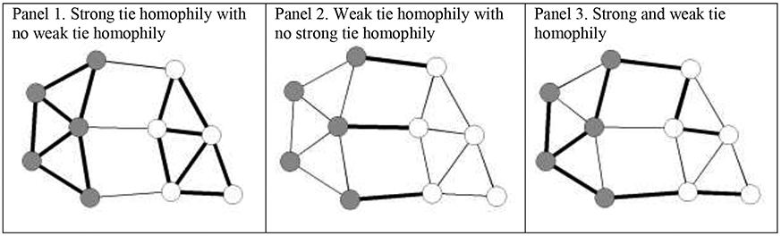
Variations in strong and weak tie homophily. Nodes are shaded according to their attribute group. The thickness of ties indicates the edge weight.

A long tradition of social science theory suggests that homophily is more likely to define the patterns of strong ties than those of weak ties. For instance, Granovetter’s work (1973) on weak ties implies that homophily is intrinsically associated with tie strength. Granovetter argues that strong ties tend to connect clusters of nodes that are characterized by transitivity, or repeated connections. Due to this redundancy, actors linked by strong ties tend to share many attributes in common, hold similar opinions, and spend time in the same geographic areas. Weak ties, on the other hand, are applauded for their ability to bridge networks by connecting actors from disparate groups with access to different types of information and opportunities. Feld (1981) further argues that individuals who are affiliated with the same activities, places, and groups are less likely to be connected by weak, bridging ties since their shared foci should lead them to develop more intimate connections. Instead, bridging ties are expected to connect pairs who share no common foci, resulting in weak connections between actors with dissimilar individual-level attributes.

Some empirical work suggests that patterns of homophily on certain individual-level characteristics may be more pronounced for ties defined by strong, intimate connections than weaker bonds. Using data on college students’ phone calls and text messages, for example, Mollgaard and colleagues (2016) find that pairs who interact regularly tend to smoke and drink alcohol at similar rates. At the same time, weaker ties characterized by less frequent communication had lower odds of connecting students with the same substance use patterns. Previous egocentric network research similarly finds that adults are more likely to share hobbies and interests with their close friends than their more distant contacts (Curry and Dunbar 2013). Taken together, these patterns carry implications for the diffusion of information and behaviors. Weak ties that link heterogenous pairs can serve as liaisons that introduce individuals to a variety of new behaviors, ranging from leisure activities to risky types of delinquency (Kreager and Haynie 2011).

Other social networks are apt to be defined by a second scenario where there are observable patterns of weak tie homophily, but processes of strong tie homophily are nonexistent (see Figure 1, Panel 2). Note that the network presented in Panel 2 includes the same set of actors and patterns of edges as the network presented in Panel 1; however, the distribution of tie weights varies across the two scenarios. In Panel 2, weaker ties tend to connect individuals who report similar traits on an attribute of interest, while homophily processes are not able to explain the patterns of stronger ties. Instead, strong ties tend to connect heterogeneous pairs of actors.

Previous empirical work finds that some networks are defined by weak tie homophily, but not strong tie homophily, for certain individual-level traits of interest. Using data on the communication patterns of mobile phone users, for example, Palchykov and colleagues (2012) report that young adults are more likely to have different-gender, rather than same-gender, “best friends,” which they define as those pairs that interact at the highest frequencies. Meanwhile, the second, third, and later “best friendships” of these young people tend to be characterized by high levels of gender homophily. Mollgaard and colleagues (2016) uncover similar patterns in a network of college students; strong ties defined by high frequencies of interaction are more likely to connect different-gender pairs, while weaker ties tend to connect same-gender dyads. Both studies argue that the gender heterophily observed in young adults’ strong ties results from the growing importance of heterosexual romantic relationships in young adulthood. Outside of gender homophily, other work finds that weak ties tend to link pairs from the same geographic neighborhood, while this is not necessarily the case for strong ties. For example, Facebook friendships are more likely to connect college students who live in the same neighborhood, rather than pairs residing in different geographic areas (Wimmer and Lewis 2010). Yet when friendships are restricted to include only pairs who were tagged together in photos, which the authors define as a more intimate bond, this geographic homophily is no longer significant.

Finally, a third scenario of interest occurs in networks that are simultaneously characterized by both strong and weak tie homophily (see Figure 1, Panel 3). Here, homophily characterizes all relationships, regardless of tie strength, and both strong and weak ties are more likely to connect those nodes that are similar. Under this scenario, differentiating between patterns of strong and weak ties is unlikely to provide additional insight. For example, the email networks of many corporations are likely be defined by both strong and weak tie homophily according to the local offices where employees work (Kleinbaum, Stuart, and Tushman 2013). Employees are apt to send more emails to colleagues who work in their same office, regardless of whether these ties are defined by daily contact or occasional interactions.

Given these various possibilities, distinguishing between strong and weak tie homophily has the potential to uncover new insights about social processes since strong and weak ties carry different consequences for the individuals they connect. Previous work finds convincing evidence that individuals tend to form pro-social bonds that are defined by racial homophily, for instance, and these patterns are understood to result in detrimental consequences for racial minorities (e.g., Goodreau, Kitts, and Morris 2009; Joyner and Kao 2000; Moody 2001). However, by differentiating between the racial homophily that defines strong versus weak ties, we are apt to gain additional insight into the ways our relational structures can both reproduce and challenge broader systems of social inequality. Strong tie racial homophily may be beneficial for minority individuals, given that strong ties are more supportive and such connections are apt to play a beneficial role when navigating discrimination and other challenges minority groups encounter in white-dominated institutions (Ibarra 1993). Weak tie racial homophily, however, may not serve this same purpose. Instead, individuals belonging to minority groups may gain access to beneficial information or novel opportunities from weak ties to white peers. Weak ties serve as bridges that can encourage the spread of new information across disparate groups and break down social barriers (Granovetter 1973; Kreager and Haynie 2011).

Despite the different implications for strong and weak tie homophily, previous work almost exclusively treats the social process as a one-dimensional process. Either all relationships are defined by homophily on a characteristic of interest, or the process does not shape any patterns of tie formation. However, by making these generalizations, we may overlook important variations in the relational phenomena that guide our social world. Most notably, there may exist scenarios where strong and weak tie homophily operate in opposite directions. In other words, while strong ties may tend to connect similar-attribute pairs, weak ties may tend to connect those with heterogeneous characteristics. Failing to differentiate between strong and weak tie homophily precludes researchers from considering how these variations shape social outcomes of interest.

In the current project, I argue that there is both theoretical and empirical value in differentiating between strong and weak tie homophily. To demonstrate this, I develop new parameters to account for these two distinct processes that can be incorporated into valued exponential random graph models (ERGMs). Then, I apply these methods to analyze a set of simulated social networks, as well as an empirical adolescent friendship network from the PROSPER study (Spoth et al. 2007).

Exponential random graph models (ERGMs) and homophily

Through the implementation of exponential random graph models (ERGMs), social network researchers have uncovered informative insights about social processes such as mutuality, triadic closure, and homophily (e.g., Felmlee and Faris 2016; Goodreau et al. 2009; McMillan 2019). ERGMs employ a statistical analysis that compares the dyadic, or pairwise, patterns observed in an actual network to what would be expected by random chance (Hunter 2007; Robins et al. 2007). By making this comparison, ERGMs can determine whether the network processes observed in an actual network are statistically significantly different from what would be expected to occur randomly.

While traditional ERGMs are limited by their ability to analyze binary, or unweighted networks, recent scholarship generalizes the ERGM to allow for the incorporation of edge weights (Desmarais and Cranmer 2012; Krivitsky 2012).¹ The valued ERGM follows a similar statistical process as the binary ERGM, which allows it to maintain much of the traditional, binary ERGM’s flexibility (Krivitsky 2012). However, there are two key differences between binary and valued ERGMs that are important to note (Krivitsky and Butts 2018). First, valued ERGMs compare the weight values of the observed network to a support, or sample space of all the possible values each dyad can take. Since the edges of binary networks can only take on a value of 0 or 1, the sample space for binary ERGMs is always a finite number of networks. For valued ERGMs, however, the set of weighted graphs is often infinite, even when the range of edge values is known. Second, valued ERGMs require the researcher to specify a reference distribution to model the distribution of tie weights. Possible reference distributions include the binomial and Poisson distributions.

More specifically, the valued ERGM for count data is defined as follows:

$$P(\mathbf{Y}=\mathit{y})=\frac{h(y)\text{exp}[{\theta }^{T}g(\mathit{y})]}{k_h(\theta )},\mathit{y}\in y.$$

Here, y is the support, and this sample space is also considered in the normalizing factor of the valued ERGM (k_h (θ)). The value of the h function depends on the reference distribution. Note that h(y) = 1 for the binary ERGM because it relies on a discrete uniform distribution.

Parameters for measuring homophily

Measures applied in previous work:

Previous research introduces various terms for measuring homophily in an ERGM framework. By including these parameters, a researcher can systematically measure the tendency for actors to report ties to other actors with whom they share a specific discrete or categorical attribute in common, while controlling for all other terms included in the model. One of the most commonly used homophily measures, and what I focus on here, is known as the nodematch parameter in the ERGM framework (Hunter et al. 2008). In binary ERGMs, the standard, uniform version of this homophily parameter is a statistic that equals the number of dyads that connect actors who belong to the same category for the specified attribute. The term’s coefficient reflects the odds that a tie will connect two actors who share an attribute category in common.²

There exist similar parameters for valued ERGMs that can capture tendencies towards homophily in weighted networks. Here, I focus on two forms of these parameters that can be implemented into valued ERGMs with relative ease. The first homophily term, which I refer to as the nonzero form, operates in a similar manner to the homophily parameter for binary ERGMs. The statistic equals the number of dyads that connect actors of the same attribute category whenever the tie’s weight is greater than zero (i.e., a tie is present). The second homophily term, or the sum form, begins to incorporate information about the edges’ weights. The sum variant of the parameter equals the sum of all tie weights that connect same-attribute actors. When the term’s coefficient is positive, it suggests that tie strength is positively associated with homophily on the attribute of interest. However, the sum form of the homophily parameter does not allow researchers to test for the presence of strong and weak tie homophily simultaneously, nor does it enable them to determine whether the strengths of these processes vary.

New measures for strong and weak tie homophily:

In the current project, I introduce two new measures that can be incorporated into valued ERGMs to differentiate between tendencies towards, or away from, homophily among strong and weak ties. I label the first term as the strong tie homophily parameter and the second as the weak tie homophily parameter. Both work in a similar manner as the nonzero form of the homophily parameter for valued ERGMs by adding one to the statistic each time there is a tie between two same-attribute individuals. However, the statistic for the strong tie homophily parameter only counts those edges with a weight greater than or equal to a value specified by the user, while the weak tie homophily parameter considers edges with a weight that is less than the specified value, but greater than zero. In other words, when the strong tie homophily parameter is positive and significant, this suggests that ties defined by higher weights are more likely to connect individuals who share an attribute of interest in common. A positive and significant coefficient for the weak tie homophily parameter suggests that low-weighted ties connect actors with similar characteristics more than would be expected to occur by chance.³

My proposed set of parameters enables a researcher to test specifically whether processes of homophily vary according to tie strength in directed or undirected networks with quantitative edge weights. Unlike the existing homophily measures, the strong and weak tie homophily terms enable one to test whether tendencies towards or away from homophily differ for strong versus weak ties. Most notably, the two measures introduced here can be included in the same valued ERGM to test for processes of strong and weak tie homophily simultaneously.

Evaluations

Simulating networks

Next, I test whether the strong and weak tie homophily parameters can uncover substantively different findings regarding tendencies towards or away from homogeneity when compared to more traditional homophily measures. To do this, I first generate a set of random networks in which there is a known clustering structure with regards to a discrete attribute. I vary my random networks according to the level of clustering on the attribute of interest and the degree to which homogenous ties are characterized by high or low weight values. By allowing for these variations, I can determine when differentiating between strong and weak tie homophily is apt to uncover novel insight. Thus, my evaluation of random networks is designed to answer two research questions. First, within what types of networks do traditional homophily measures prevent researchers from uncovering differences in the magnitude of strong versus weak tie homophily? Second, within what types of networks do traditional homophily measures prevent researchers from uncovering differences in the direction of strong versus weak tie homophily?

All of my simulated networks consist of 45 nodes that are assigned to one of three categories of a discrete attribute (groups 1, 2, and 3). Attribute assignments are distributed so that there is an equal number of nodes belonging to each category (15 nodes per category). All edges are directed, and each network has a density of roughly 10%. For the purpose of this project, edges can take on a weight of either 1 or 2. In other words, a tie with a weight of 2 can be conceptualized as a strong tie, while a tie characterized by a weight of 1 can be understood as a weaker tie. While some types of relationships are characterized by a broader range of variation in tie strength, there exist many examples of observed data that categorizes ties into two ranked categories. For instance, previous research distinguishes between Facebook friends who are tagged together in photos and those who are not (Wimmer and Lewis 2010), as well as close versus extended kin (Verdery et al. 2012) and members of a couple’s wedding party versus wedding invitees (Berry 2006).

Next, I vary the simulated networks according to two factors: (1) the amount of clustering within the attribute groups and (2) the degree to which homogenous ties are characterized by high- versus low-weight values. I consider four variations in the level of clustering among attribute groups. First, I simulate a set of networks with high clustering in which the vast majority, or roughly 80%, of edges connect same-attribute actor pairs, regardless of their weight. The second set of networks is defined by medium clustering in which about two thirds of ties link pairs who share a common attribute, while one third connect cross-attribute dyads. The third set is defined by low clustering. Here, each actor is connected to a roughly equal number of same-attribute and different-attribute peers, but due to the fact that there are three distinct groups, most actors have more within-group ties than would be expected by random chance. The final set of networks is characterized by no clustering, meaning that actors are equally likely to report ties to same- versus cross-attribute peers. In this scenario, about one third of ties link same-attribute nodes, while the remaining two thirds connect cross-attribute pairs.

Within each level of clustering, I consider five possible variations in the distribution of tie weights: (1) 95% of ties connecting same-attribute pairs are assigned a weight of 2 versus 5% of cross-attribute pairs, (2) 80% of same-attribute pairs are assigned a weight of 2 versus 20% of cross-attribute pairs, (3) 50% of same-attribute and 50% of cross-attribute pairs are assigned a weight of 2, (4) 20% of same-attribute and 80% of cross-attribute ties are assigned a weight of 2, and (5) 5% of same-attribute and 95% of cross-attribute ties are assigned a weight of 2. All ties that are not assigned a weight of 2 are assigned a weight of 1. Note that scenarios 1 and 2 are defined by strong tie homophily, but less weak tie homophily. Scenarios 4 and 5 are defined by weak tie homophily, but less strong tie homophily. Other than the aforementioned structural variations, I assume no further structural tendencies in my simulated networks.

In sum, my evaluation of simulated networks can be understood as 4 × 5 computational experiment consisting of 20 scenarios that vary according to the level of clustering and the relationship between homophily and tie strength. Within each of the 20 scenarios, I simulate 100 networks, resulting in a total of 2,000 random networks. I present descriptive statistics that summarize the 2,000 random networks in Table 1 and plot examples of several networks in Figure 2.

Table 1.

Descriptive statistics for simulated networks (n = 2,000).

Level of Clustering	Density	Outdegree	Within-Group Outdegree	Between-Group Outdegree
High Clustering	0.097 (0.006)	4.259 (0.270)	3.504 (0.241)	0.742 (0.134)
Medium Clustering	0.097 (0.006)	4.252 (0.274)	2.781 (0.233)	1.465 (0.164)
Low Clustering	0.098 (0.007)	4.293 (0.296)	2.077 (0.226)	2.215 (0.189)
No Clustering	0.099 (0.007)	4.360 (0.296)	1.384 (0.174)	2.974 (0.237)
Percent of Strong Ties Within & Between Groups			Average Within Group Tie Weight	Average Between Group Tie Weight
95% Within, 5% Between			1.952 (0.024)	1.057 (0.031)
80% Within, 20% Between			1.815 (0.045)	1.203 (0.060)
50% Within, 50% Between			1.510 (0.061)	1.501 (0.069)
20% Within, 80% Between			1.185 (0.045)	1.797 (0.060)
5% Within, 95% Between			1.048 (0.024)	1.943 (0.031)

Notes: For each level of clustering, descriptive statistics reflect averages across all tie distributions. For each tie distribution scenario, descriptive statistics reflect averages across all clustering levels. Standard deviations are presented in parentheses.

Figure 2.

Examples of simulated networks by clustering level and tie distribution. Nodes are shaded according to their attribute group. Tie thickness indicates edge weight.

Plan of analysis and comparison to traditional homophily measures

For each simulated network, I first estimate a valued ERGM that incorporates both the strong and weak tie homophily terms. In each of these valued ERGMs, I also include four controls to account for structural properties. First, the nonzero parameter accounts for the baseline tendency for actors to have ties, or report edges with nonzero values. Second, I include the sum parameter to control for the baseline intensity of interactions. Though both parameters’ coefficients are difficult to interpret substantively, they help account for tendencies towards or against tie formation (Kritvitsky 2012, Schoeneman, Zhu, and Desmarais 2020). Third, I include a reciprocity parameter to measure tendencies towards mutuality. I specify this term to sum together the minimum tie value of each mutual dyad that appears in the observed network (following Krivitsky and Butts 2018). Finally, I include a transitivity term to account for patterns of triadic closure. For this parameter, it is necessary to determine three criteria that generalize the notion of transitivity to patterns of weighted edges. To measure the intensity of the two-path that represents the required preconditions for a transitive triad to form (e.g., a → b, b → c), I take the minimum value of each edge weight in the two-path. Next, I consider the maximum value of all two paths between node a and node c that do not include node b, and finally, I take the minimum value of tie weights connecting nodes a and c. Collectively, these criteria are understood to represent the most conservative tests for triadic closure (Krivitsky and Butts 2018). Note that all valued ERGMs apply a binomial distribution as their reference distribution.

To determine under which circumstances there is substantive utility in differentiating between strong and weak tie homophily, I estimate two sets of valued ERGMs that incorporate standard homophily terms for analyzing ordinal network data. The first utilizes the nonzero form of the homophily parameter, while the second incorporates the sum form. Both sets of valued ERGMs include the same terms to account for reciprocity, transitivity, and the tendency to form edges, and also apply a binomial distribution as their reference distribution.

Meta-analysis:

Given the large number of simulated networks, it was necessary to run valued ERGMs on each of the networks separately. After models reached adequate convergence (goodness of fit statistics and diagnostic tests available in the Supplemental Materials, Part A), I aggregated the findings for each of the three sets of valued ERGMs by employing a two-level random effects meta-analysis. Following previous work (e.g., Snijders and Baerveldt 2003), I calculate the sample-wide mean for each ERGM coefficient by estimating a random intercept model where I fix the level-one variance to equal the coefficient’s squared standard error and the network serves as the second level. This averaging process takes into account the different levels of precision across all models by giving greater weight to those with more precise estimates (see Lubbers and Snijders 2007).

Simulation results

For most of the simulated networks, I find evidence that differentiating between strong and weak tie homophily can uncover new insights about the tendencies towards or away from homogamy in social relationships. I demonstrate this in Figure 3, where each panel presents results from the ERGM meta-analyses according to the distributions of edge weights across the random networks. All x-axes indicate the level of within-group clustering and the y-axes report the size of the ERGM coefficient of interest. I plot values of the observed coefficients for each ERGM homophily parameter separately (i.e., weak tie homophily, strong tie homophily, nonzero form of standard homophily, sum form of standard homophily). Tables that present coefficients for all observed ERGM meta-analyses are presented in the Supplemental Materials (Part B).

Figure 3:

Meta-analysis results for ERGM homophily coefficients by level of clustering and tie weight ratio. Each panel represents a different distribution of tie weights, with the proportion of within group and between group strong ties presented above each panel. The horizontal axis indicates the level of clustering by group, regardless of tie weight.

When the distribution of strong and weak ties is equal across the edges that link same-attribute and cross-attribute actors (e.g., the middle pane of Figure 3), the four homophily coefficients are nearly identical within each level of clustering. For example, in the high clustering scenario, the strong tie homophily coefficient is 2.59 and the weak tie homophily coefficient is 2.56. This implies that when compared to random chance, same-attribute pairs are significantly more likely to be connected, regardless of whether the tie is associated with a high or low weight. The size of the strong and weak tie homophily coefficients is also comparable to those of the standard ERGM parameters under this scenario (nonzero form = 2.57, sum form = 1.61). All previously mentioned homophily coefficients are statistically significant at p < 0.001.⁴

As the distribution of strong and weak ties begins to differ across the edges that link same- versus cross-actor pairs, the strong and weak tie homophily terms are able to uncover variations in the tendency towards homogamy. For example, in the medium clustering networks, the strong tie homophily coefficient is negative and statistically significant (b = −1.34, p < 0.001) when the vast majority of same-attribute connections are defined as weak ties (see Figure 3, Panel 5). Yet when same-attribute connections are almost exclusively defined as strong ties, this same coefficient takes a value of 4.33 and is statistically significant at the p < 0.001 level in the medium clustering networks (see Panel 1). This means that, across networks with the same exact clustering structure, the odds that a strong tie will connect two same-attribute actors can vary from being significantly less likely to significantly more likely than would be expected by random chance. Note that traditional ERGM homophily parameters are unable to detect this variation. For example, the homophily coefficients for the nonzero variant of the standard homophily term is roughly 1.5 across the medium clustering networks, regardless of the distribution of edge weights.

The importance of differentiating between strong and weak tie homophily becomes even more imperative as the amount of clustering decreases. For example, in the no clustering scenario where 80% of same-attribute ties are defined by strong connections while only 20% of cross-attribute links are characterized by higher weights, the strong tie homophily coefficient is positive and the weak tie homophily coefficient is negative (Figure 3, Panel 4). In the reverse scenario where 20% of edges between same-attribute pairs are strong ties while 80% of crossgroup pairs are defined by high weights, the strong tie homophily coefficient is negative in direction, while the weak tie homophily coefficient is positive (Figure 3, Panel 2). These results are noteworthy since the commonly-used ERGM terms cannot pick up on this difference in direction.

Empirical example: PROSPER adolescent friendship network

Next, I apply these techniques to examine patterns of gender and racial homophily in an empirical network from the Promoting School-Community Partnerships to Enhance Resilience (PROSPER) study. The study collected panel data on over 50 socio-centric adolescent friendship networks from dozens of public school districts in rural and semi-rural Midwestern communities (for more details on the study, see Spoth et al. 2007). To demonstrate the utility of my strong and weak tie homophily measures, the current study focuses on a single network from the study that represents a cohort of 140 eighth graders who attended the same middle school (see Figure 4).

Figure 4.

Friendship network of eight graders in a middle school. Thickness of ties represents the strength of each edge. Node shape indicates gender, node color indicates race.

Directed friendship networks were created from a survey item that asked students, “who are your best and closest friends in your grade?” Respondents could nominate up to two best friends and five other friends. For the current project, I define best friend nominations as strong ties (edge weight = 2) and other friend nominations as weak ties (edge weight = 1).⁵ To test whether this tie strength is associated with gender or racial homophily, I construct a binary, actor-level variable for gender where 1 = boy and a variable for race that uses two survey items asked at each wave of the survey. First, respondents were asked if they identified as Hispanic or Latino. Then, they were asked to select a racial category that best described them from “Native American/American Indian,” “Black/African American,” “Asian,” “white,” “more than one of those listed,” and “other.” Given the low amount of racial diversity in the school (roughly 83% of students identified as white), it was necessary to recode race into two categories: 0 = white and non-Hispanic/Latino and 1 = racial minority (following previous work that analyzes the PROSPER data, e.g., Osgood et al. 2014).

To test for strong and weak tie homophily on race and gender, I begin by estimating a valued ERGM that includes the nonzero form of the standard homophily parameter to test for patterns of racial and gender homogamy. Then, I estimate two additional valued ERGMs, one tests for strong and weak tie racial homophily using my proposed set of measures, while the other does so for gender homophily. In both models, the cut points for these parameters are set such that the strong tie homophily parameter considers patterns of best friendships, while the weak tie homophily parameter measures other, non-best friendships.

All ERGMs apply a binomial distribution as their reference distribution and include controls for tendencies towards the formation of edges, reciprocity, and transitivity. I also control for socio-economic (SES) homogamy using a nonzero form of the standard homophily parameter because previous work finds that people tend to be tied to those of similar SES backgrounds and this intertwines with patterns of racial homophily (McPherson et al. 2001, Moody 2001). Since the in-school PROSPER survey did not ask respondents to report their parents’ highest education level or household income, I construct a proxy, binary measure of SES using a survey item that asks respondents whether they receive free or reduced school lunch (1 = receives free or reduced lunch) (following Osgood et al. 2014).

Empirical example: Results

When standard homophily terms are applied to measure racial and gender homophily in the adolescent friendship network, the coefficient for gender homophily is positive and significant (b = 1.32, p < 0.001), indicating a strong tendency towards the formation of same-gender best and other friendships (see Table 2, Model 1). The coefficient for racial homophily, on the other hand, does not reach statistical significance (b = −0.02, p = 0.74), suggesting that friendships connect same-race peers as frequently as would be expected by random chance. While this finding contradicts the general patterns documented in previous literature, it is important to note that tendencies toward racial homophily are often minimal in contexts defined by low levels of racial heterogeneity (Moody 2001), such as the school considered here.

Table 2.

Valued ERGM results for a PROSPER friendship network.

	Model 1		Model 2		Model 3
	b	SE	b	SE	b	SE
Racial homophily	−0.025	(0.070)			0.066	(0.063)
Strong tie racial homophily			0.323	(0.108) **
Weak tie racial homophily			−0.131	(0.079)
Gender homophily	1.319	(0.137) ***	1.373	(0.116) ***
Strong tie gender homophily					1.010	(0.225) ***
Weak tie gender homophily					1.512	(0.149) ***
SES homophily	0.047	(0.076)	0.043	(0.080)	0.075	(0.050)
Reciprocity	2.854	(0.140) ***	2.798	(0.127) ***	2.825	(0.128) ***
Transitivity	0.779	(0.055) ***	0.739	(0.051) ***	0.763	(0.128) ***
Nonzero	−4.913	(0.166) ***	−4.507	(0.212) ***	−5.577	(0.371) ***
Sum	−1.327	(0.102) ***	−1.620	(0.161) ***	−0.877	(0.266) ***
AIC	−39913		−40043		−39911
BIC	−39858		−39980		−39848

Notes:

^***p < 0.001

^**p < 0.01

^*p < 0.05. S.E. refers to standard error. The minimum form of the reciprocity parameter and the maximum, minimum, maximum form of the transitivity parameter are used.

Different patterns emerge, however, when strong and weak tie racial homophily are considered separately (Table 2, Model 2). The coefficient for strong tie racial homophily is positive and significant (b = 0.32, p < 0.01), suggesting that individuals are more likely to nominate same-race peers as their best friends than would be expected by random chance. However, this same pattern does not define patterns of the weaker friendship ties; the weak tie homophily coefficient is negative, although not significant (b = −0.13, p = 0.10). In other words, non-best, other friendships do not connect same-race peers more frequently than would be expected in the friendship network.

When strong and weak tie gender homophily are considered, I find evidence that both processes guide patterns of adolescent friendship (b = 1.01, p < 0.001 and b = 1.51, p < 0.001, respectively) (Table 2, Model 3). These results suggest that adolescents are more likely to nominate same-gender peers as best and other friends than would be expected after accounting for all controls in the model. Note that the coefficient for the strong tie homophily parameter is about 50% greater than the weak tie homophily coefficient, which suggests that strong and weak tie homophily may operate at different magnitudes of strength in this network. However, supplemental analyses demonstrate that this difference is not statistically significant at the p < 0.05 level (see Supplemental Materials, Part C).

Discussion

When the social connections of a network can be defined as either strong or weak, I argue that it is meaningful to consider the association between tie strength and homophily. For example, in some networks, patterns of strong ties are apt to be guided by a tendency towards homophily on the attribute of interest, while those of weak ties are shaped by different processes. At the same time, there exist scenarios where networks should be defined by weak tie homophily, even when strong ties tend to connect heterogeneous pairs. Traditional ERGM homophily parameters preclude researchers from unpacking these variations, which limits their ability to uncover meaningful insights about social outcomes of interest.

Here, I propose a new set of measures that can simultaneously test for strong and weak tie homophily within a valued ERGM framework. I compare my proposed set of measures with two commonly used homophily terms by analyzing a set of 2,000 randomly simulated networks that vary in their distribution of tie weights and level of within-group clustering. My evaluations demonstrate that differentiating between strong and weak tie homophily can provide new insights about various network configurations. This is particularly the case when there are low levels of clustering on the attribute on interest. In the most extreme scenarios, for example, traditional ERGM terms will suggest a positive and significant tendency towards general homophily, when in fact this phenomenon is being driven entirely by patterns of either strong or weak ties. In such a network, ties of one level of strength will be more likely to connect same-attribute peers, while the other type will link similar actors less frequently than would be expected by random chance. When there are higher levels of clustering on the attribute of interest, differentiating between strong and weak tie homophily can enable researchers to uncover variations in the magnitude of homophily for high- versus low-value ties, but they are less likely to observe differences in direction. Thus, traditional techniques for measuring homophily can obscure the association between homophily and tie strength, making it important to consider how processes of strong and weak tie homophily operate simultaneously.

By allowing the simulated networks to vary according to the distribution of tie weights and level of within-group clustering, this project aims to make recommendations of best practices for measuring homophily in social networks. Overall, I advise researchers with two-level, ordinal network data to consider how individual-level attributes shape network patterns of strong and weak ties differently. Making this distinction is apt to uncover novel patterns, especially when theory or empirical evidence suggests that a network’s strong and weak ties carry different implications for individual-level outcomes or broader group processes. Furthermore, differentiating between strong and weak tie homophily is particularly crucial when traditional ERGM coefficients for homophily are estimated to be small in size (e.g., coefficient values less than 1). This is because when clustering on the attribute of interest is low, it is increasingly plausible that strong and weak tie homophily operate in substantively different ways.

The techniques I propose for measuring strong and weak tie homophily have the potential to inform a range of substantive research. As demonstrated in my empirical example, tendencies towards strong and weak tie homophily can vary in terms of both their magnitude and direction. For instance, in my sample of adolescents, friendships are more likely to connect same-gender peers, regardless of their strength. However, an adolescent’s odds of reporting a same-gender weak tie are slightly greater than their odds of reporting a same-gender strong tie, though this difference is not statistically significant. Given that adolescence is a period in the life course when heterosexual dating becomes increasingly common, these variations in strong and weak tie homophily likely result from respondents nominating their significant others as best friends (Mollgaard et al. 2016; Palchykov et al. 2012).

At the same time, strong ties were significantly more likely to connect same-race adolescent pairs than would be expected by chance, while this tendency did not shape the formation of weaker friendship ties. Shared racial background may be crucial for facilitating the high levels of social and emotional support that define strong ties (Homans 1950; Ibarra 1993), while weak ties that cross different racial groups could be beneficial for adolescents. This is because connections that link cross-race peers have the potential to introduce the involved actors to new opportunities and ideas (Granovetter 1973). In sum, this example suggests that the welldocumented patterns of racial homophily may operate differently for strong versus weak bonds of adolescent friendship.

There are many ways that future research could extend upon the concepts of strong and weak tie homophily that I introduce here. For instance, one limitation of the measures I present is that they can only consider homophily for two types of ties: those that are defined as strong and those that are defined as weak. Although there are many datasets that define interactions in this manner (for examples, see McMillan et al. 2018; Osgood et al. 2014; Wimmer and Lewis 2010), there also exist networks where edges are defined by large ranges of continuous values. Future research would benefit from extending these analyses to model networks with wider distributions of tie weights. For instance, higher order polynomials of the sum form of the general homophily parameter could be created to capture the continuous associations between tie strength and the odds of forming same-attribute ties. Additionally, future theoretical and methodological work should consider how other structural processes are shaped by the distribution of edge weights, such as reciprocity, transitivity, and degree skew. For example, it is unknown whether patterns of mutuality vary when members of a dyad send strong versus weak ties. Future research could apply the same approach used here to study how strong and weak ties operate differently for other local network structures of interest.

While homophily on key actor-level attributes characterizes many types of social relationships (McPherson et al. 2001), it is unclear whether these processes differ for strong versus weak ties, and what the consequences of this variation entail. Making such distinctions is crucial, however, because we know that strong and weak relational ties carry different implications. Strong ties tend to be characterized by greater levels of social support, while weak ties are more likely to circulate new information and inspire change (Burt 2004; Granovetter 1973; Kreager and Haynie 2011). Thus, distinguishing between strong and weak tie homophily should help us unpack the individual- and group-level implications of homogenous relationships, such as when the phenomena can bring positive, pro-social benefits versus when it exacerbates inequalities. The concepts of strong and weak tie homophily can bring these variations further to light, as well as provide new theoretical and empirical insight about the association between tie strength and homogeneity.

Highlights.

• Important to consider the association between homophily and tie strength

• Defines concepts of strong and weak tie homophily and proposes associated ERGM terms

• Analyzes random, simulated networks and an empirical adolescent friendship network

• Strong and weak tie homophily operate at different magnitudes in most networks

• Some networks are defined by strong tie homophily and no weak tie homophily, or vice versa

References

- Berry Brent. 2006. “Friends for Better or for Worse: Interracial friendship in the United States as Seen through Wedding Party Photos.” Demography 43(3):491–510. [DOI] [PubMed] [Google Scholar]
- Borgatti Stephen P., Everett Martin G., and Johnson Jeffery C.. 2018. Analyzing Social Networks. Los Angeles, CA: Sage Publications. [Google Scholar]
- Burt Ronald S. 2004. “Structural Holes and Good Ideas.” American Journal of Sociology 110: 349–399. [Google Scholar]
- Cook James M. 2000. “The Social Structure of Political Behavior: Action, Interaction and Congressional Cosponsorship.” Unpublished doctoral diss., Univ. Ariz., Tucson, AZ. [Google Scholar]
- Curry Oliver, and Dunbar Robin I. M.. 2013. “Do Birds of a Feather Flock Together? The Relationship between Similarity and Altruism in Social Networks.” Human Nature 24: 336–347. [DOI] [PubMed] [Google Scholar]
- Davies Huw T. O., Crombie Iain K., and Tavakoli Manouche. 1998. “When Can Odds Ratios Mislead?” BMJ 316:989. [DOI] [PMC free article] [PubMed] [Google Scholar]
- Desmarais Bruce A., and Cranmer Skyler J.. 2012. “Statistical Inference for Valued-Edge Networks: The Generalized Exponential Random Graph Model.” PLoS One 7(1):e30136. [DOI] [PMC free article] [PubMed] [Google Scholar]
- Duxbury Scott W. 2020. “Dealing with Unobserved Heterogeneity in Exponential Random Graph Models.” Presented at the Annual Meeting of the American Sociological Association. August 2020. San Francisco, CA. [Google Scholar]
- Feld Scott L. 1981. “The Focused Organization of Social Ties.” American Journal of Sociology 86(5):1015–1035. [Google Scholar]
- Felmlee Diane and Faris Robert. 2016. “Toxic Ties: A Network of Friendship, Dating, and Cyber Victimization.” Social Psychology Quarterly 79: 243–262. [Google Scholar]
- Granovetter Mark S. 1973. “The Strength of Weak Ties.” American Journal of Sociology 78(6):1360–1380. [Google Scholar]
- Goodreau Steven M., Kitts James A., and Morris Martina. 2009. “Birds of a Feather, or Friend of a Friend? Using Exponential Random Graph Models to Investigate Adolescent Social Networks.” Demography 46(1): 103–125. [DOI] [PMC free article] [PubMed] [Google Scholar]
- Homans George C. 1950. The Human Group. New York: Harcourt, Brace & World. [Google Scholar]
- Hunter David R. 2007. “Curved Exponential Family Models for Social Networks.” Social Networks 29: 216–230. [DOI] [PMC free article] [PubMed] [Google Scholar]
- Hunter David R., Handcock Mark S., Butts Carter T., Goodreau Steven M., and Morris Martina. 2008. “ergm: A Package to Fit, Simulate and Diagnose Exponential-Family Models for Networks.” Journal of Statistical Software 24(3):1–29. [DOI] [PMC free article] [PubMed] [Google Scholar]
- Joyner Kara, and Kao Grace. 2000. “School Racial Composition and Adolescent Racial Homophily.” Social Science Quarterly 81(3):810–825. [Google Scholar]
- Kleinbaum Adam M., Stuart Toby E., and Tushamn Michael L.. 2013. “Discretion Within Constraint: Homophily and Structure in a Formal Organization.” Organization Science 24(5): 1316–1336. [Google Scholar]
- Kreager Derek A., and Haynie Dana L.. 2011. “Dangerous Liaisons? Dating and Drinking Diffusion in Adolescent Peer Networks.” American Sociological Review 76(5): 737–763. [DOI] [PMC free article] [PubMed] [Google Scholar]
- Krivitsky Pavel N. 2012. “Exponential-Family Graph Models for Valued Networks.” Electronic Journal of Statistics 6: 1100–1128. [DOI] [PMC free article] [PubMed] [Google Scholar]
- Krivitsky Pavel N., and Butts Carter T.. 2018. “Modeling Valued Networks with statnet.” [Google Scholar]
- Lubbers Miranda J., and Snijders Tom A.B.. 2007. “A Comparison of Various Approaches to the Exponential Random Graph Model: A Reanalysis of 102 Student Networks in School Classes.” Social Networks 29(4): 489–507. [Google Scholar]
- Maoz Zeev. 2012. “Preferential Attachment, Homophily, and the Structure of International Networks, 1816–2003.” Conflict Management and Peace Science 29(3): 341–369. [Google Scholar]
- McMillan Cassie. 2019. “Tied Together: Adolescent Friendship Networks, Immigrant Status, and Health Outcomes.” Demography 56(3):1075–1103. [DOI] [PMC free article] [PubMed] [Google Scholar]
- McMillan Cassie, Felmlee Diane, and Wayne Osgood D. 2018. “Peer Influence, Friend Selection, and Gender: How Network Processes Shape Adolescent Smoking, Drinking, and Delinquency.” Social Networks 55: 86–96. [DOI] [PMC free article] [PubMed] [Google Scholar]
- Miler McPherson, Smith-Lovin Lynn, and Cook James M.. 2001. “Birds of a Feather: Homophily in Social Networks.” Annual Review of Sociology 27: 415–444. [Google Scholar]
- Mollgaard Anders, Zettler Ingo, Dammeyer Jesper, Jensen Mogens H., Lehmann Sune, and Mathiesen Joachim. 2016. “Measure of Node Similarity in Multilayer Networks.” PLoS One 11(6): e0157436. [DOI] [PMC free article] [PubMed] [Google Scholar]
- Moody James. 2001. “Race, School Integration, and Friendship Segregation in America.” American Journal of Sociology 107: 679–716. [Google Scholar]
- Moreno Jacob L. 1934. Who Shall Survive? A New Approach to the Problem of Human Interrelations. Washington, D.C.: Nervous and Mental Disease Publishing Co. [Google Scholar]
- Onnela Jukka-Pekka, Saramaki Jari, Hyvonen Jorkki, Szabo Gabor, Lazer David, Kaski Kimmo, Kertész Janos, and Barabasi Albert-László. 2007. “Structure and Tie Strengths in Mobile Communication Networks.” Proceedings of the National Academy of Science 104(18):7332–7336. [DOI] [PMC free article] [PubMed] [Google Scholar]
- Opsahl Tore, Agneessens Filip, and Skvoretz John. 2010. “Node Centrality in Weighted Networks: Generalizing Degree and Shortest Paths.” Social Networks 32(3):245–251. [Google Scholar]
- Osgood D. Wayne, Feinberg Mark E., Wallace Lacey, and Moody James. 2014. “Friendship Group Position and Substance Use.” Addictive Behaviors 39(5): 923–933 [DOI] [PMC free article] [PubMed] [Google Scholar]
- Palchykov Vasyl, Kaski Kimmo, Kertesz Janos, Barabási Albert-Laszlo, and Dunbar Robin I. M.. 2012. “Sex Differences in Intimate Relationships.” Scientific Reports 2(37): 1–5. [DOI] [PMC free article] [PubMed] [Google Scholar]
- Robins Gary, Pattison Pip, Kalish Yuval, and Lusher Dean. 2007. “An Introduction to Exponential Random Graph (p*) Models for Social Networks.” Social Networks 29(2): 173–191. [Google Scholar]
- Saul Zachary M., and Filkov Vladimir. 2007. “Exploring Biological Network Structure Using Exponential Random Graph Models.” Bioinformatics 23(19): 2604–2611. [DOI] [PubMed] [Google Scholar]
- Schoeneman John, Zhu Boliang, and Desmarais Bruce A.. 2020. “Complex Dependence in Foreign Direct Investment: Network Theory and Empirical Analysis.” Political Science Research and Methods doi: 10.1017/psrm.2020.45. [DOI] [Google Scholar]
- Snijders Tom A. B., and Baerveldt Chris. 2003. “A Multilevel Network Study of the Effects of Delinquent Behavior on Friendship Evolution.” The Journal of Mathematical Sociology, 27 (2-3): 123–151. [Google Scholar]
- Spoth Richard, Redmond Cleve, Shin Chungyeol, Greenberg Mark, Clair Scott, and Feinberg Mark. 2007. “Substance-Use Outcomes at 18 Months Past Baseline: The PROPSER Community-University Partnership Trial” American Journal of Preventive Medicine 32(5): 395–402. [DOI] [PMC free article] [PubMed] [Google Scholar]
- Stehlé Juliette, Charbonnier François, Picard Tristan, Cattuto Ciro, and Barrat Alain. 2013. “Gender Homophily from Spatial Behavior in a Primary School: A Sociometric Study.” Social Networks 35(4): 604–613. [Google Scholar]
- Verdery Ashton M., Entwisle Barbara, Faust Katherine, and Rindfuss Ronald R.. 2012. “Social and Spatial Networks: Kinship Distance and Dwelling Unit Proximity in Rural Thailand.” Social Networks 34(1): 112–127. [DOI] [PMC free article] [PubMed] [Google Scholar]
- Wang Yishu, Fang Huaying, Yang Dejie, Zhao Hongyu, and Deng Minghua. 2019. “Network clustering analysis using mixture exponential-family random graph models and its application in genetic interaction data.” IEEE/ACM Transactions on Computational Biology and Bioinformatics 16(5): 1743–1752. [DOI] [PubMed] [Google Scholar]
- Wimmer Andreas, and Lewis Kevin. 2010. “Beyond and Below Racial Homophily: ERG Models of a Friendship Network Documented on Facebook.” American Journal of Sociology 116(2): 583–642. [DOI] [PubMed] [Google Scholar]
Associated Data
This section collects any data citations, data availability statements, or supplementary materials included in this article.