Supervised clustering of high-dimensional data using regularized mixture modeling

Abstract

Identifying relationships between genetic variations and their clinical presentations has been challenged by the heterogeneous causes of a disease. It is imperative to unveil the relationship between the high-dimensional genetic manifestations and the clinical presentations, while taking into account the possible heterogeneity of the study subjects.We proposed a novel supervised clustering algorithm using penalized mixture regression model, called component-wise sparse mixture regression (CSMR), to deal with the challenges in studying the heterogeneous relationships between high-dimensional genetic features and a phenotype. The algorithm was adapted from the classification expectation maximization algorithm, which offers a novel supervised solution to the clustering problem, with substantial improvement on both the computational efficiency and biological interpretability. Experimental evaluation on simulated benchmark datasets demonstrated that the CSMR can accurately identify the subspaces on which subset of features are explanatory to the response variables, and it outperformed the baseline methods. Application of CSMR on a drug sensitivity dataset again demonstrated the superior performance of CSMR over the others, where CSMR is powerful in recapitulating the distinct subgroups hidden in the pool of cell lines with regards to their coping mechanisms to different drugs. CSMR represents a big data analysis tool with the potential to resolve the complexity of translating the clinical representations of the disease to the real causes underpinning it. We believe that it will bring new understanding to the molecular basis of a disease and could be of special relevance in the growing field of personalized medicine.

Introduction

Detection and estimation of the genetic markers associated with phenotypic features is one of the most important problems in biomedical research. Predictive models have been extensively used to link genetic markers to a phenotypic trait; however, the unobserved patient heterogeneity obfuscates the effort to build a unified model that works for all hidden disease subtypes. It has been well understood that various subtypes exist for many common diseases, which vary in etiology, pathogenesis and prognosis [1–3]. For example, the cancer cells are constantly evolving in the tumor microenvironment, and they may acquire variations on alternative pathways in response to treatment, which explains why certain patients have better prognoses than others in response to the same treatment [4, 5]. This implies that the same predictive model that links genetic markers to a phenotypic trait may not be valid for every patient, and further it is unclear to what extent the patients should be considered together [6]. Therefore, it is judicious to construct a set of heterogeneous models, each of which corresponds to one subtype.

The fast advancement in high-throughput technology has transformed the biomedical research ecosystem by scaling data acquisition, providing us with unprecedented opportunity to interrogate biology in novel and creative ways. For cancer research, the Broad Institute Cancer Cell Line Encyclopedia (CCLE) [7], Cancer Therapy Response Portal v1/v2 [8] and Genomics of Drug Sensitivity in Cancer [9] datasets contain 24, 185, 481 and 261 drug compound screening data for 504, 242, 860 and 1001 cell lines, respectively, together with the multi-omic profiles of the cell lines; the Cancer Genome Atlas has collected biospecimens and matched clinical phenotypes for over 10 000 cancer patients [10]. Consequently, for each sample, there is a tremendous amount and variety of data: 20 000 genes’ expression profiles, 1 million single-nucleotide polymorphism genotypes, exome and whole-genome sequences, methylation of tens of thousands of CpG islands and the expression of microRNA. From this plurality of data, we anticipate that exploratory methods will serve to extract and characterize genetic subgroups relevant to phenotypic outcomes. However, the growing number of variables does not necessarily increase the discriminative power in classification [11]. To identify the most important genetic biomarkers, variable selection is one of the most commonly used approaches. In particular, various regularization methods have received a great deal of attention [12–15]. Despite major progress in the research of penalized regression, heterogeneity in variable selection of high-dimensional feature spaces remains challenging.

Unsupervised learning algorithms that are typically employed to deal with heterogeneity in subpopulations include finite mixture models by assuming a separate distribution for each subpopulation [16–19] and bi-clustering-based discrete algorithms that perform feature selection and sample clustering simultaneously [20–22]. Based on the resultant genetic subtypes, deeper investigation into the genetic and phenotypic distinctions within each subtype could be carried out. Although the clustering methods may produce satisfactory classification of subtypes, many methods do not select genetic markers distinctive for each subtype, which however is essential in precision medicine. In addition, in the unsupervised clustering of high-dimensional omics data, the high-dimensional genetic feature space may give rise to many different ways of clustering the samples, which may or may not be biologically/clinically meaningful [5]. Usually, the relevance of the subtypes to external biological or clinical presentations is analyzed in a post hoc fashion. As a result, without any supervision, the defined clusters based on a sea of genetic features may not necessarily relate to the phenotype of interest. Existing supervised clustering methods apply an ad hoc two-stage approach that consists of feature selection based on association with an external biological or clinical response variable and clustering of samples using the selected features. However, due to the heterogeneity in sample population, the relationship between the external variable and the individual features could be highly non-linear, and a pre-selection of the features is not optimal.

Hence, in order to find sample subgroups guided by an external response variable, which carries important biological/clinical information, we need to perform clustering of the samples and regression of the response on the features at the same time. Clearly, our challenges are distinct in two ways: the variables of interest to each subgroup may be a distinct and sparse set of the high-dimensional genetic features, and the set of patients in each subgroup is not known a priori. In this article, we proposed a novel and efficient supervised clustering algorithm based on penalized mixture regression model that handles the subject heterogeneity in high-dimensional regression setting. Essentially, we assume that observations belong to unlabeled classes with class-specific regression models relating their unique and selective genetic markers to the phenotypic outcome. The ultimate goal is to group the subjects into clusters such that the observed response variables conditional on the feature variables in the same cluster are more similar to each other than those from different clusters. In other words, we are detecting sample clusters such that in the same cluster, the relationship between the features and the response could be described by one unified model, which differs from another cluster.

Preliminaries

Since first introduced in [23], finite mixture Gaussian regression (FMGR) has been extensively studied and widely used in various fields [16, 24–28]. Let , be a finite set of observations, the design matrix with intercept and independent variables and the response vector. Consider an FMGR model parameterized by , it is assumed that when the -th observation, , belongs to the k-th component, , then , and . In other words, the conditional density of given is , where is the normal density function with mean and variance . Moreover, the log-likelihood for observations is

(1)

Unfortunately, the maximum likelihood estimator (MLE) for (1) is not well defined in this case. A fundamental problem with the MLE computation is that the global maximum of the mixture likelihood does not exist, as the likelihood function is not bounded. Obviously, if we let the variance of one component go to 0, the value of the likelihood function goes to infinity. To circumvent this problem, we introduce restrictions on the variance parameters such that, , and following the practice of [29, 30], we define as

where is a very small positive value. Similar to [31], we set to be 0.01. Throughout the rest of the article, we always assume such a constrained formulation of maximum-likelihood estimation.

Note that the maximizer of (1) does not have an explicit solution and is usually solved by the expectation–maximization (EM) algorithm. Basically, the EM algorithm maximizes the complete log-likelihood function, , through iterative steps, which is defined by

(2)

where is a binary latent cluster indicator variable and if the -th observation belongs to the -th cluster, and 0 otherwise. The EM algorithm iterates between the following two steps:

E-step: computing the conditional expectation of with respect to given the current estimates , where denotes the parameter estimate at the -th iteration for and denotes the parameter provided at initialization. The conditional expectation, denoted as , is

Then the conditional expectation of at the current step is given by

M-step: maximizing with respect to , i.e.

where denotes the parameter space of as .

While the mixture regression model is capable of handling the heterogeneous relationships, it does not work in the case of high-dimensional genetic features, where the total number of parameters to be estimated is far more than the total number of observations. In addition, with the dense linear coefficients given by the ordinary EM algorithm, it is hard to deduce the disease subtype-specific genetic markers and make meaningful interpretations.

Penalized mixture regression has been explored in different settings [32–36] to handle the high-dimensional mixture regression problem. The variable selection problem in sthe finite mixture of regression model was first studied using regularization methods such as LASSO [12] and SCAD [14] in [32]. They considered the traditional cases when the number of candidate covariates is much smaller than the sample size and proposed a modified EM algorithm to perform both estimation and variable selection simultaneously. The following methods consider the cases where the number of covariates may be much larger than the sample size. In [33], the authors proposed a reparameterized mixture regression model and showed evidence for the benefit of the reparameterized model with numerically better behaviors. A block-wise minorization maximization (MM) algorithm was proposed in [35], where at each iteration, the likelihood function is maximized with respect to a block of variables while the rest of the blocks are held fixed. The work proposed by Devijver [37] mainly considers the parameter estimation, after the variables have been selected by -penalized MLE, as well as model selection among a set of pre-given ones. The imputation-conditional consistency (ICC) algorithm proposed by [36] adopted a two-stage approach: variable selection by aggregating the selection results through multiple EM iterations and the parameter estimation stage for which the problem could be cast as a low-dimensional one.

While some of the methods may produce consistent estimates of under proper conditions, they tend to suffer from slow convergence rate in high-dimensional setting, especially with smaller or larger , and the number of hyperparameters for regularization further drags down the computational efficiency caused by the need of cross-validation. We here propose a novel algorithm based on classification EM for penalized mixture regression to circumvent these existing challenges in clustering high-dimensional data using mixture regression, which largely increased the computational efficiency.

The rest of the article is organized as follows: in Section 3, we introduce our algorithm, component-wise sparse mixture regression (CSMR); in Section 4, we compare CSMR with five state-of-the-art algorithms on synthetic datasets, namely, LASSO, Ridge regression, random forest (RF), ICC [36] and FMRS [32]; in Section 5, we applied all the algorithms on 24 drug sensitivity data in CCLE, to screen for genes that underlie the heterogeneous drug resistance mechanisms.

Methods

We assume that the samples belong to different subpopulations, each of which is defined by a distinct relationship between the genetic biomarkers and the phenotype of interest, and the genetic markers are sparse subsets of the high-dimensional genetic profiles specific to each subpopulation. Figure 1 illustrated an example where the patients fall under two distinct subgroups: blue for patients acquiring one mechanism to the treatment that resulted in responsiveness, while pink for patients acquiring another mechanism to the same drug that resulted in non-responsiveness. The goal of our method is to cluster the samples (blue and pink) supervised by the patients drug sensitivity measure and find the defining genetic features (yellow) associated with each cluster. The identified genetic features could be further studied to guide targeted therapeutic designs.

Figure 1.

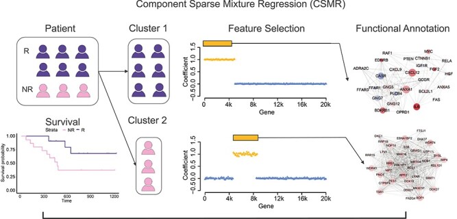
The motivation of CSMR. Under the same treatment, some patients acquired one mechanism to deal with the drug, (blue), while others picked up another (pink), resulting in different prognoses for the same treatment. The motivation of CSMR is to cluster the patients in a supervised fashion and examine what are the genes (yellow) that are selected in tumor progression that lead to the different drug resistance subtypes of patients, and their functions (network).

The penalized likelihood of mixture regression

Knowing that is sparse means many elements in will tend to be close to zero but not exactly zero without proper regularization in the model. To simultaneously shrink the insignificant regression coefficients in and estimate , we could introduce a penalty term to (1) and optimize the following penalized log-likelihood function:

(3)

where denotes the observed log-likelihood and is a regularizer of the regression coefficients; the penalty for each component is dependent on a component specific hyperparameter . Various types of penalty forms were used in the mixture regression model, and we could consider the LASSO penalty form as it is convex and thus advantageous for numerical computation [32, 33, 36], i.e.

(4)

where is usually chosen among 0, 0.5, 1 as in [33]. A non-zero would involve in the penalty term that could largely increase the computational complexity in the maximization step in using EM algorithm [32, 33].

Similar to the case of low-dimensional mixture regression, the EM algorithm could be adopted by maximizing the penalized complete log-likelihood function defined as , as in existing methods. The conditional expectation corresponding to the penalized likelihood function is given by

(5)

In the E step, the conditional expectation of is similar to the low-dimensional case. However, in the M step, maximizing with respect to is more complicated than the low-dimensional case. The involvement of in makes it impossible to obtain nice closed form solutions for neither of the two. We next discuss the use of a variant of EM algorithm that could largely increase the computational efficiency.

The classification EM algorithm

The classification EM (CEM) algrorithm is a variant of the EM algorithm. It has been popularly used in the finite Gaussian mixture model [38, 39] and shown to be have faster convergence rate [40]. Basically, the latent variables define a partition s.t. iff . Within each iteration, instead of using weighted least square estimation in the M step as in the EM algorithm, CEM estimates the component-wise parameters using all observations within each hard partition. The CEM algorithm maximizes through iterating among three steps:

E-Step: compute conditional expectation, , similar to the traditional EM algorithm.

C-Step: disentangle the observations into clusters, by assigning as the set of observations most likely in cluster , i.e. . Let denote the total number of observations in cluster .

M-Step: parameter estimation within each disentangled cluster, where is estimated as and are simply estimated as the ordinary least square (OLS) estimators using observations in only.

The biggest advantage of the CEM algorithm is that it disentangles the mixture into individual non-overlapping components, such that flexible sparsity control could be easily achievable within each component. Hence, for the high-dimensional mixture regression problem, we could simply replace the OLS estimator in the M step of the CEM algorithm by a sparse estimator, i.e.

This is simply regularized linear regression, for which many efficient algorithms exist [41]. Note that when , the involvement of in the penalty term makes it challenging for the maximization with regards to both and . Maximizing the function with regards to the mixing proportions is much more complex than maximizing its leading term, i.e. , and in our CSMR algorithm, for simplicity, we ignored the penalty term involving ’s, i.e. , when solving for , such that it will have a nice closed form solution. Moreover, it has been shown to work well in [32] and our own simulation data. As for the solution of , we show in the next section that under the proposed CEM updates, the involvement of s only affects the scale of s, which are selected with cross-validation within each iteration and hence does not impact the estimation of .

The CSMR algorithm

Here we proposed the CSMR algorithm to solve the high-dimensional mixture regression problem based on the CEM algorithm. In CSMR, the mixture regression setting could handle the hidden cluster problem, and the disentangled clusters under CEM could efficiently solve the feature selection problem in a high-dimensional setting. At the E-step, we calculate the posterior probability similar to traditional EM algorithm; at the C-step, we assign each observation to a cluster that it most likely belongs to, similar to traditional CEM; at the M-step, for each component, we perform regularized linear regression to obtain a sparse set of non-zero coefficients.

A big challenge with the penalized mixture regression problem is the choice of component specific penalty parameters . The s are related to the amount of regularization, and their selection is a critical issue in a penalized likelihood approach. It is usually based on a trade-off between bias and variance: large values of tuning parameters tend to select a simple model whose parameter estimates have smaller variance, whereas small values of the tuning parameters lead to complex models, with smaller bias. Cross-validation over a grid search is the commonly adopted method to select the optimal combination of , but this becomes increasingly prohibitive with the increase of , especially when we do not have a good knowledge of the theoretical range of the .

Hence, instead of first performing penalized linear regression for given and then searching for the optimal combination of [32], we propose to conduct the tuning of with cross-validation inside the CEM iterations. Specifically, under the CEM algorithm, all the components are disentangled, we could hence perform hyperparameter tuning inside each iteration within each component. This is to say, at the M-step, we not only estimate the regression coefficients but also find the best tuning parameter for the component. Hence, at the end of the algorithm, we avoid the hyperparameter tuning, as they have already been selected within the iteration. We adopted the efficient cross-validation algorithm for selecting the optimal regularization parameter under regularized linear regression [41]. Since we no longer need to run the algorithm multiple times on a -dimensional grid space of the penalty parameters, we could hence largely reduce the computational cost. We have shown in simulation studies that penalty parameters selected this way empirically worked very well.

Another adaptation on the traditional CEM algorithm of CSMR is a model refit step following the CEM steps. To increase the numerical stability and achieve faster convergence, at the end of each iteration, we refit the mixture regression model using flexible EM algorithm with only the selected variables of each component. Basically, for each component, the coefficients of the variables not selected at the M-step will be forced to be zero. This could be easily achievable by allowing only the selected variables of component to enter into the model fitting of the -th regression parameters.

The CSMR algorithm requires the initialized values . Here, we order the features based on its individual Pearson correlation with the response variable and then fit a low-dimensional mixture regression model solved by the traditional EM algorithm using the top correlated genes. CSMR is implemented in R and was made available in https://github.com/zcslab/CSMR.

Selection of component number

The number of clusters is a sensible parameter because it describes the heterogeneity of the population. For selection of , we could use a modified BIC criterior that minimizes

where represents the parameter estimates for and is the effective number of parameters to be estimated, similar to [42]. Specifically, there are standard deviations, , associated with the regression lines; component proportions, , since ; and all the non-zero linear regression coefficients for all the components.

In addition to the BIC criteria, we also offer a cross-validation algorithm for the selection of . Take a 5-fold cross-validation as an example. For given , at each repetition, 80% samples are used for training to obtain the regularized parameter . Then, for a sample drawn from the 20% testing samples, its cluster membership, , is first predicted as

Here, denotes the CSMR estimated parameters when the number of components is . After assigning the observation to component , we could make prediction of the response based on linear regression, i.e. , as well as the associated residual, . Notably, such a prediction of the response is different from simple linear regression, as the prediction process requires knowing the value of the response, in order to assign it to the right cluster. After knowing its cluster membership, a prediction of the response could be made.

A large will tend to overfit the data with a more complex model of higher variance, while smaller might select a simpler model with larger bias. Using the independent testing data, we could decide how to balance the trade-off between bias and variance. To evaluate how the estimated model under explains the testing data, we could calculate the root-mean-square-error between and or Pearson correlation between the two. By repeating this procedure multiple times, a more robust and stable evaluation of the choice of should be derived based on the summarized RMSE or Pearson correlations.

Application to simulation data

Data generation procedure

To simulate observations with independent variables, we first simulated the design matrix , such that the 1st column of is all 1, corresponding to the intercept, i.e. ; and for the rest of the columns, all the elements follow i.i.d. standard normal distribution, i.e. . The component proportions were made to be equal, i.e. . For component , a random sample of size was taken from the set , denoted as , to mimic the sparse component-specific variables predictive of the response. Moreover, we simulated the component specific coefficients, , to be a random draw from , if ; and let , if .

The response variable was generated by the following two-step process:

1. Draw the component indicator variable following the multinomial distribution , in other words, .

2. Draw an observation according to a normal distribution , if .

Here, we fix . We explored the performances of existing methods under 15 different simulation scenarios, for each of which, 100 repetitions were conducted: Cases 1–3. Cases 4–6. Cases 7–9. Cases 10–12. Cases 13–15.

Baseline methods

We compared CSMR with five different methods, including penalized regression, or LASSO; penalized regression, or Ridge regression (RIDGE); RF-based regression; sparse mixture regression, FMRS [43]; and the ICC algorithm [36]. They differ in their ability to perform prediction, clustering and variable selection, as shown in Table 1.

Table 1.

Baseline methods

	Prediction	Clustering	Variable selection
CSMR
LASSO
RIDGE
RF
FMRS
ICC

Among them, CSMR, ICC and FMRS are all capable of doing variable selection at the same time as sample clustering. However, FMRS can only deal with relatively lower dimensional features, while ICC represents the method that is powerful in dealing with much higher dimensional features.

Performance comparisons

We focused on four metrics for method comparisons: (1) the average correlation between predicted and observed response; (2) the true positive rate (TPR) and (3) true negative rate (TNR) of variable selection; and (4) the rand index (RI) of sample clustering. Note that for observation , its predicted response is given by , where is its cluster membership indicator. The average of the four metrics over 100 simulations in each scenario was calculated and shown in Table 2. Here, we assume that the true is known.

Table 2.

Comparisons of CSMR with other five methods in various simulation settings

Metrics
	Experiment
	Parameter	2	3	4	0.5	1	2	200	300	400	5	8	20	100	500	2000
	CSMR	0.994	0.988	0.999	0.998	0.994	0.977	0.987	0.993	0.994	0.994	0.995	0.992	0.994	0.994	0.951
	ICC	0.984	0.985	0.909	0.998	0.984	0.982	0.992	0.992	0.984	0.984	0.994	0.992	0.984	0.994	0.993
	LASSO	0.778	0.654	0.585	0.745	0.778	0.729	0.776	0.756	0.778	0.778	0.754	0.743	0.778	0.799	0.779
	RIDGE	0.789	0.697	0.639	0.783	0.789	0.772	0.834	0.802	0.789	0.789	0.782	0.784	0.789	0.885	0.955
	RF	0.605	0.583	0.487	0.719	0.605	0.700	0.717	0.720	0.605	0.605	0.691	0.716	0.605	0.804	1
	FMRS	0.706	0.676	0.568	0.780	0.706	0.769	0.727	0.797	0.706	0.706	0.780	0.780	0.706	0.143	-
Variable	CSMR	0.980	0.950	0.538	1	0.980	1	0.956	1	0.980	0.980	0.998	0.999	0.980	1	0.900
Selection	ICC	0.461	0.332	0.339	0.500	0.461	0.500	0.500	0.500	0.461	0.461	0.496	0.500	0.461	0.500	0.500
(TPR)	FMRS	0.579	0.552	0.487	0.681	0.579	0.674	0.672	0.706	0.579	0.579	0.635	0.679	0.579	0.700	-
Variable	CSMR	0.992	0.976	0.785	0.994	0.992	0.968	0.966	0.990	0.992	0.992	0.992	0.993	0.992	0.998	1
Selection	ICC	0.870	0.957	0.669	0.973	0.870	0.735	0.966	0.972	0.870	0.870	0.953	0.972	0.870	0.994	0.998
(TNR)	FMRS	0.512	0.680	0.758	0.504	0.512	0.500	0.502	0.506	0.512	0.512	0.515	0.499	0.512	0.502	-
Sample	CSMR	0.917	0.833	0.624	0.943	0.917	0.787	0.852	0.886	0.917	0.917	0.908	0.893	0.917	0.865	0.869
Clustering	ICC	0.879	0.838	0.549	0.941	0.879	0.787	0.878	0.881	0.879	0.879	0.903	0.887	0.879	0.856	0.886
(RI)	FMRS	0.513	0.546	0.624	0.502	0.513	0.502	0.501	0.501	0.513	0.513	0.502	0.501	0.513	0.502	-

The bold values indicate the best performance among all methods being compared.

In general, CSMR performs the best in terms of the four evaluation metrics in the majority of the scenarios. For prediction accuracy of the response using correlation, CSMR and ICC perform comparably well and CSMR slightly better in most of the cases. This is expected as LASSO, RIDGE and RF cannot deal with the sample heterogeneity and FMRS does not work well when the feature dimension is high. In particular, FMRS failed to converge for . For sensitivity and specificity of the variable selection, CSMR performs significantly better than ICC and FMRS. Selection of the correct variables is very important as it characterizes the unique features of each component, based on which, we could further deduce the biological interpretation of each unique component. ICC and FMRS suffer from very low sensitivity of variable selection in almost all cases, and their specificity metrics are not desirable either. For clustering, CSMR again has the best or close to the best performance compared with ICC and FMRS. ICC achieved similar performance with CSMR in some cases, but it clearly suffers when or the number of true predictors becomes large. We also compared the computational efficiency of CSMR and ICC under the parameter setting: or 4. Figure 2 shows the computational cost and its standard deviation for two algorithms over 100 repetitions. Clearly, the computational efficiency of ICC drops significantly when increases from 2 to 4, while the time consumption for CSMR stays approximately the same.

Figure 2.

Time consumption of CSMR, and ICC on simulation data for (left) and (right), and over 100 repetitions; error bars indicate standard deviations.

Hence, from simulation data, we could see that CSMR achieved the most desirable performance in terms of prediction accuracy, variable selection and clustering, compared with three non-mixture regularized models, and two regularized mixture regression models. While ICC is competitive in some cases, it severely suffers from poor variable selection, and its computational cost is too prohibitive compared with CSMR.

In ICC, by treating the clustering membership as missing data, each iteration step automatically selects a distinct set of variables, inducing a Markov chain, and ICC ‘aggregates’ the variables selected after burn-in steps to get the final sparse set of variables. In contrast, FMRS does variable selection for fixed hyperparameter set, and by searching among a grid of the hyperparameter sets, the variables are selected that corresponds to the hyperparameter set with the best variance-bias trade-off. CSMR inherited the advantages of both ICC and FMRS in that it conducts variable selection within each iteration step by automatically tuning the hyperparameters , saving the computational cost of large scale selection of , which increases exponentially with . In addition, the highly efficient built-in cross-validation step within the CEM iterations could largely increase the sensitivity and specificity of the variable selection procedure, and the flexible model refitting step following the CEM steps guarantees that the algorithm could achieve faster convergence and more stable results.

Application to CCLE data

Description of the dataset

Over the past three decades, the use of genetic data to inform drug discovery and development pipeline has generated huge excitement. Predicting the drug sensitivity becomes an integral part of the precision health initiative. Although earlier efforts successfully identified many new drug targets, the overall clinical efficacy of the developed drugs has remained unimpressive, owing in large part to the population heterogeneity, that is, different patients may have different disease causing factors and hence drug targets. Here, we apply CSMR to study the patient heterogeneity in their response to different drug treatments and select the most key genetic features that underlie the heterogeneous disease causes.

We collected gene expression data of 470 cell lines on 7902 genes, as well as the cell lines’ sensitivity score to all 24 drugs, from the CCLE dataset [7]. The sensitivity score, also called the AUCC score, is defined as the area above the fitted dose response curve, and it has been shown to have better predictive accuracy of sensitivity to targeted therapeutic strategies than other measures, such as IC50 or EC50 [44]. We applied all five methods on the dataset, where the drug sensitivity score was treated as the response variable and the gene expressions as independent variables. Here, FMRS is not applicable as the feature dimension is too high while the sample size is too small; hence, it is omitted from further analysis. Our goal is to study the biological mechanism of possible heterogeneity in drug sensitivity, under the hypothesis that cells exhibit subgroup characteristics by selecting different genes that confer their different levels of drug sensitivity.

Results

We compare the performances of the five methods using cross-validation. Basically, for each drug, we conduct a 5-fold cross-validation by holding 80% of the data as training, and 20% as testing data, for each of the 100 repetitions. At each repetition, the 20% testing data is used to independently evaluate the performance of each method. At the training phase, we start by fixing the hyperparameters involved in all methods. The penalty parameters for LASSO and RIDGE were selected by cross-validation within the training samples. For RF, the default parameters were used in the function ‘randomForest’ of the package with the same name. For ICC, we used the selected component number as in its original paper [36]. For CSMR, to select the best , we performed both cross-validation and the traditional BIC criteria introduced in Methods, over a grid of . We adopted the results from cross-validation, as there is a lack of rigorous theoretical foundation for the validity of the traditional BIC under this high-dimensional setting, and the data-driven selection of cross-validation seems more reasonable. The selected for BIC and cross-validation using CSMR and used for ICC is summarized in Supplementary Table S1. With the hyperparameters fixed, we then conduct parameter estimations for each of the five methods using the training samples and conclude the training phase.

At the testing phase, the predicted and true drug sensitivity scores were examined in terms of their correlation, and residual mean squared error (RMSE). Note that to our knowledge this part of the testing data has never been used in the hyperparameter tuning or parameter estimation previously. The distributions of RMSE and correlations over 100 repetitions for all the 24 drugs for all the five methods were shown in Figure 3 and Supplementary Figure S1, respectively. For 22 drugs, CSMR had the significantly smaller average RMSE and was very close to the smallest RMSE for the rest of the two drugs, and we could make the same conclusions based on the correlation results as well. This demonstrated the consistent and robust performance of CSMR over the others.

Figure 3.

The distributions of the RMSE over 100 repetitions for the five methods, for the 24 drugs. The lower the RMSE value, the better the performance. ‘C’,‘I’,‘A’,‘G’ and ‘F’ stand for ‘CSMR’,‘ICC’,‘LASSO’,‘RIDGE’ and ‘Random Forest’.

Among the five methods, RF had the poorest performance on the testing data, probably caused by model overfitting. LASSO and RIDGE worked much better than RF, probably due to its power in model selection. However, they performed significantly worse than ICC and CSMR in the majority of the cases, which indicates the existence of population heterogeneity and necessity of using mixture modeling. The performance of ICC is much worse than CSMR in most of the cases, which we believe is caused by the underestimation of the population heterogeneity by ICC. In other words, the selection of in ICC is too conservative. In fact, according to cross-validation, the number of distinct clusters given by CSMR for the drugs is either 3 or 4, while for ICC, the number of distinct clusters are determined to be less than 3 for half of the drugs. We believe that cross-validation is a data-driven approach for selection of and should be more reasonable than theoretically derived criteria. In the case of CCLE data, the samples are different types of cells from very different experimental and genetic backgrounds, and it is expected that they would pick up different molecular mechanisms to deal with the attacks of the drugs. Hence, the cluster number given by CSMR is more realistic than ICC. It is note that for those drugs that CSMR and ICC gave the same number of distinct clusters, namely Irinotecan, L-685458, Lapatinib, Paclitaxel, PD-0332991, PHA-665752 and TKI258; CSMR exhibited much smaller RMSE than ICC.

Figure 4 demonstrated the Venn diagram of the selected genes for different components for each drug, and all the selected genes could be found in Supplementary Table S2. It could be seen that for the same drug, different clusters of cells indeed acquire different coping mechanisms, as seen by the different set of genes selected. This again confirms the high heterogeneous populations within the CCLE cohort. For each drug, we pooled all the selected genes together and conducted pathway enrichment analysis against 1328 pathways collected in [45], and the top enriched pathways are shown in Supplementary Figure S2. Again, it could be seen that different responses to different drugs have been employed.

Figure 4.

For each drug, the Venn diagram of the selected genes for different mixing components is shown. The numbers show the size of overlap among the gene sets.

Conclusions

With the recent rapid evolution in genomic technologies, we have now entered a new phase, one in which it is possible to comprehensively characterize the genetic profiles of large population of subjects. Importantly, the development of sequencing technologies has been paired with a transition towards integrating genetic data with phenotypic data, such as in electronic medical records. Such a synergy has the potential to ultimately facilitate the generation of a data commons useful for identifying relationships between genetic variations and their clinical presentations. Unfortunately, existing big data analysis tools for mining the information rich data commons have not been very impressive with regards to the overall translational or clinical efficacy, owing in large part to the heterogeneous causes of disease. It is hence imperative to unveil the relationship between the genetic variations and the clinical presentations, while taking into account the possible heterogeneity of the study subjects.

In this paper, we proposed a novel supervised clustering algorithm using penalized mixture regression model, called CSMR, to deal with the challenges in studying the heterogeneous relationships between high-dimensional genetic features and a phenotype that serves as a response variable to guide the clustering. CSMR is capable of simultaneous stratification of the sample population and sparse feature-wise characterization of the subgroups. The algorithm was adapted from the classification EM algorithm, which offers a novel supervised solution to the clustering problem, with substantial improvement on both the computational efficiency and biological interpretability. Experimental evaluation on simulated benchmark datasets with different settings demonstrated that the CSMR can accurately identify the subspaces on which a subset of features are explanatory to the response variables and the feature characteristics of the subspaces, and it outperformed the baseline methods. Application of CSMR on the heterogeneous CCLE dataset demonstrated the superior performance of CSMR over the others. On the CCLE dataset, CSMR is powerful in recapitulating the distinct subgroups hidden in the pool of cell lines with regards to their coping mechanisms to different drugs. CSMR also demonstrated the uniqueness of different subgroups for the same drug, as seen by the distinctly selected genes for the subgroups.

In summary, CSMR represents a big data analysis tool with the potential to bridge the gap between advancements in biotechnology and our understanding of the disease and resolve the complexity of translating the clinical representations of the disease to the real causes underpinning it. We believe that such a tool will bring new understanding to the molecular basis of a disease and could be of special relevance in the growing field of personalized medicine.

Key Points

• Detecting genetic markers associated with phenotypes is crucial; however, existing predictive models have been challenged by disease heterogeneity. While unsupervised learning can deal with heterogeneity, the defined clusters may not necessarily relate to the phenotype of interest.

• We proposed a supervised clustering algorithm based on the regularized mixture regression model, which handles the high-dimensional genetic features, and greatly improved the computational efficiency over others. Specifically, it efficiently performs clustering, feature selection and hyperparameter tuning in the same process.

• Evaluation on both simulated datasets and a real expression dataset for 500 cell lines and 24 drugs demonstrated the superior performance of our algorithm over the others. Particularly, our algorithm is powerful in recapitulating the distinct subgroups hidden in the pool of cell lines with regards to their coping mechanisms to different drugs.

• Our algorithm represents a big data analysis tool with the potential to resolve the complexity of translating the clinical representations of the disease to the real causes underpinning it. It has special relevance in the growing field of personalized medicine.

Wennan Chang is a PhD student in the Department of Electrical and Computer Engineering, Purdue University.

Changlin Wan is a PhD student in the Department of Electrical and Computer Engineering, Purdue University.

Yong Zang is an assistant professor in the Department of Biostatistics and a member of the Center for Computational Biology and Bioinformatics, Indiana University School of Medicine.

Chi Zhang is an assistant professor in the Department of Medical and Molecular Genetics and a member of the Center for Computational Biology and Bioinformatics, Indiana University School of Medicine.

Sha Cao is an assistant professor in the Department of Biostatistics and a member of the Center for Computational Biology and Bioinformatics, Indiana University School of Medicine.

References

- 1. Curtis C, Shah SP, Chin SF, et al. The genomic and transcriptomic architecture of 2,000 breast tumours reveals novel subgroups. Nature 2012; 486(7403): 346–52. [DOI] [PMC free article] [PubMed] [Google Scholar]
- 2. Schlicker A, Beran G, Chresta CM, et al. Subtypes of primary colorectal tumors correlate with response to targeted treatment in colorectal cell lines. BMC Med Genomics 2012; 5(1): 66. [DOI] [PMC free article] [PubMed] [Google Scholar]
- 3. Guinney J, Dienstmann R, Wang X, et al. The consensus molecular subtypes of colorectal cancer. Nat Med 2015; 21(11): 1350–6. [DOI] [PMC free article] [PubMed] [Google Scholar]
- 4. Marusyk A, Polyak K. Tumor heterogeneity: causes and consequences. Biochim Biophys Acta Rev Cancer 2010; 1805(1): 105–17. [DOI] [PMC free article] [PubMed] [Google Scholar]
- 5. Cao S, Chang W, Wan C, et al. Bi-clustering based biological and clinical characterization of colorectal cancer in complementary to cms classification. bioRxiv 508275, 2018. [Google Scholar]
- 6. Köbel M, Kalloger SE, Boyd N, et al. Ovarian carcinoma subtypes are different diseases: implications for biomarker studies. PLoS Med 2008; 5(12): e232. [DOI] [PMC free article] [PubMed] [Google Scholar]
- 7. Barretina J, Caponigro G, Stransky N, et al. The cancer cell line encyclopedia enables predictive modelling of anticancer drug sensitivity. Nature 2012; 483(7391): 603–7. [DOI] [PMC free article] [PubMed] [Google Scholar]
- 8. Basu A, Bodycombe NE, Cheah JH, et al. An interactive resource to identify cancer genetic and lineage dependencies targeted by small molecules. Cell 2013; 154(5): 1151–61. [DOI] [PMC free article] [PubMed] [Google Scholar]
- 9. Yang W, Soares J, Greninger P, et al. Genomics of drug sensitivity in cancer (gdsc): a resource for therapeutic biomarker discovery in cancer cells. Nucleic Acids Res 2012; 41(D1): D955–61. [DOI] [PMC free article] [PubMed] [Google Scholar]
- 10. Weinstein JN, Collisson EA, Mills GB, et al. The cancer genome atlas pan-cancer analysis project. Nat Genet 2013; 45(10): 1113. [DOI] [PMC free article] [PubMed] [Google Scholar]
- 11. Fan J, Han F, Liu H. Challenges of big data analysis. Natl Sci Rev 2014; 1(2): 293–314. [DOI] [PMC free article] [PubMed] [Google Scholar]
- 12. Tibshirani R. Regression shrinkage and selection via the lasso. J R Stat Soc B Methodol 1996; 58(1): 267–88. [Google Scholar]
- 13. Zou H. The adaptive lasso and its oracle properties. J Am Stat Assoc 2006; 101(476): 1418–29. [Google Scholar]
- 14. Fan J, Li R. Variable selection via nonconcave penalized likelihood and its oracle properties. J Am Stat Assoc 2001; 96(456): 1348–60. [Google Scholar]
- 15. Zhang C-H, et al. Nearly unbiased variable selection under minimax concave penalty. Ann Statist 2010; 38(2): 894–942. [Google Scholar]
- 16. McLachlan GJ, Peel D. Finite Mixture Models. New York, USA: John Wiley & Sons, 2004. [Google Scholar]
- 17. Fraley C, Raftery AE. How many clusters? Which clustering method? Answers via model-based cluster analysis. Comput J 1998; 41(8): 578–88. [Google Scholar]
- 18. Fraley C, Raftery AE. Model-based clustering, discriminant analysis, and density estimation. J Am Stat Assoc 2002; 97(458): 611–31. [Google Scholar]
- 19. Wan C, Chang W, Zhang Y, et al. Ltmg: a novel statistical modeling of transcriptional expression states in single-cell rna-seq data. Nucleic Acids Res 2019; 47(18): e111–1. [DOI] [PMC free article] [PubMed] [Google Scholar]
- 20. Xie J, Ma A, Zhang Y, et al. Qubic2: a novel and robust biclustering algorithm for analyses and interpretation of large-scale rna-seq data. Bioinformatics 2020; 36(4): 1143–9. [DOI] [PMC free article] [PubMed] [Google Scholar]
- 21. Wan C, Chang W, Zhao T, et al. Fast and efficient boolean matrix factorization by geometric segmentation. In: The Thirty-Fourth AAAI Conference on Artificial Intelligence, New York, USA, 2020, 6086–93. [Google Scholar]
- 22. Wan C, Chang W, Zhao T, et al. Denoising individual bias for a fairer binary submatrix detection. In: Proceedings of the 29th ACM International Conference on Information & Knowledge Management. Online Conference. 2020, pp. 2245–8
- 23. Goldfeld S, Quandt R. The estimation of structural shifts by switching regressions. In: Annals of Economic and Social Measurement, Vol. 2, number 4. Cambridge MA, USA: NBER, 1973, 475–85. [Google Scholar]
- 24. Böhning D. Computer-Assisted Analysis of Mixtures and Applications: Meta-analysis, Disease Mapping and Others, Vol. 81. Boca Raton, Florida, USA: CRC Press, 1999. [Google Scholar]
- 25. Hennig C. Identifiablity of models for clusterwise linear regression. J Classification 2000; 17(2):273–96. [Google Scholar]
- 26. Jiang W, Tanner MA. Hierarchical mixtures-of-experts for exponential family regression models: approximation and maximum likelihood estimation. Ann Statist 1999;987–1011. [Google Scholar]
- 27. Xu L, Jordan MI. On convergence properties of the em algorithm for gaussian mixtures. Neural Comput 1996; 8(1): 129–51. [DOI] [PubMed] [Google Scholar]
- 28. Frühwirth-Schnatter S. Finite Mixture and Markov Switching Models. New York, USA: Springer Science & Business Media, 2006. [Google Scholar]
- 29. Hathaway RJ, et al. A constrained formulation of maximum-likelihood estimation for normal mixture distributions. Ann Statist 1985; 13(2): 795–800. [Google Scholar]
- 30. Hathaway RJ. A constrained em algorithm for univariate normal mixtures. J Stat Comput Simul 1986; 23(3): 211–30. [Google Scholar]
- 31. Yu C, Yao W, Chen K. A new method for robust mixture regression. Canad J Statist 2017; 45(1): 77–94. [DOI] [PMC free article] [PubMed] [Google Scholar]
- 32. Khalili A, Chen J. Variable selection in finite mixture of regression models. J Am Stat Assoc 2007; 102(479): 1025–38. [Google Scholar]
- 33. Städler N, Bühlmann P, Van De Geer S. L1-penalization for mixture regression models. Test 2010; 19(2): 209–56. [Google Scholar]
- 34. Fan J, Lv J. Comments on: L1-penalization for mixture regression models. Test 2010; 19(2): 264–9. [Google Scholar]
- 35. Lloyd-Jones LR, Nguyen HD, McLachlan GJ. A globally convergent algorithm for lasso-penalized mixture of linear regression models. Comput Statist Data Anal 2018; 119:19–38. [Google Scholar]
- 36. Li Q, Shi R, Liang F. Drug sensitivity prediction with high-dimensional mixture regression. PLoS One 2019; 14(2):e0212108. [DOI] [PMC free article] [PubMed] [Google Scholar]
- 37. Devijver E, et al. Finite mixture regression: a sparse variable selection by model selection for clustering. Electron J Stat 2015; 9(2): 2642–74. [Google Scholar]
- 38. Blömer J, Brauer S, Bujna K. Hard-clustering with gaussian mixture models. arXiv preprint arXiv:1603.06478 2016. [Google Scholar]
- 39. Celeux G, Govaert G. A classification em algorithm for clustering and two stochastic versions. Comput Statist Data Anal 1992; 14(3): 315–32. [Google Scholar]
- 40. Faria S, Soromenho G. Fitting mixtures of linear regressions. J Stat Comput Simul 2010; 80(2): 201–25. [Google Scholar]
- 41. Hastie T, Qian J. Glmnet vignette. Standford, CA: Standford University, 2016. Available from: https://mran.microsoft.com/snapshot/2017-12-11/web/packages/glmnet/vignettes/glmnet_beta.pdf. [Google Scholar]
- 42. Pan W, Shen X. Penalized model-based clustering with application to variable selection. J Mach Learn Res 2007; 8(May): 1145–64. [Google Scholar]
- 43. Khalili A, Chen J, Lin S. Feature selection in finite mixture of sparse normal linear models in high-dimensional feature space. Biostatistics 2011; 12(1): 156–72. [DOI] [PubMed] [Google Scholar]
- 44. In SJ, Neto EC, Guinney J, et al. Systematic Assessment of Analytical Methods for Drug Sensitivity Prediction from Cancer Cell Line Data. In: Biocomputing 2014. Hackensack NJ, USA: World Scientific, 2014, 63–74. [PMC free article] [PubMed] [Google Scholar]
- 45. Liberzon A, Subramanian A, Pinchback R, et al. Molecular signatures database (msigdb) 3.0. Bioinformatics 2011; 27(12): 1739–40. [DOI] [PMC free article] [PubMed] [Google Scholar]
Associated Data
This section collects any data citations, data availability statements, or supplementary materials included in this article.