Abstract
Real-world predictive models in healthcare should be evaluated in terms of discrimination, the ability to differentiate between high and low risk events, and calibration, or the accuracy of the risk estimates. Unfortunately, calibration is often neglected and only discrimination is analyzed. Calibration is crucial for personalized medicine as they play an increasing role in the decision making process. Since random forest is a popular model for many healthcare applications, we propose CaliForest, a new calibrated random forest. Unlike existing calibration methodologies, CaliForest utilizes the out-of-bag samples to avoid the explicit construction of a calibration set. We evaluated CaliForest on two risk prediction tasks obtained from the publicly-available MIMIC-III database. Evaluation on these binary prediction tasks demonstrates that CaliForest can achieve the same discriminative power as random forest while obtaining a better-calibrated model evaluated across six different metrics. CaliForest is published on the standard Python software repository and the code is openly available on Github.
Keywords: random forest, calibration, healthcare, python, Applied computing→Health informatics, General and reference→Empirical studies, Computing methodologies→Classification and regression trees, Bagging
1. INTRODUCTION
Machine learning-based predictive algorithms have been touted as the new frontier of healthcare [5, 19]. Random forest has emerged as a popular methodology due to its ability to work with a mixture of data types, handle missing data, and achieve high predictive performance [2, 4, 12, 17, 27, 32, 33]. Yet, these models are often only evaluated on discrimination, or how well the model differentiates between high risk and low risk of the event, and fail to provide any analysis of calibration. Calibration, the accuracy of the actual risk estimates, is also essential to assess the usefulness of the model [1, 28]. An accurate probability estimate is crucial for clinical decision making. For example, if a predictive model predicts a woman has a 45% chance of breast cancer, the clinician may refer her for chemo-prevention trials [10]. Well-calibrated predictive models are imperative for personalized medicine as they play an increasing role in both clinical care and translational research [14].
Unfortunately, a highly discriminative classifier (e.g., a classifier with a large area under the receiver operating characteristic (ROC) curve, or AUROC) may not be well-calibrated. Several machine learning approaches such as Naive Bayes, decision trees, and artificial neural networks have been shown to have exhibit poor calibration [3, 8, 31]. In fact, logistic regression model, a widely adopted predictive model in healthcare, may not be well-calibrated [14]. As a result, various techniques have been proposed to calibrate existing predictive models [14, 21, 31] or directly incorporate calibration in the model itself [6, 13]. Under the former approach, some of the original training examples must be set aside for the purpose of calibration. Unfortunately, in the presence of a limited number of samples (a common scenario in healthcare data), this can negatively impact the discriminative power of the predictive model in addition to the calibration function itself. Instead, an alternative approach is to extend the machine learning model itself to avoid the construction of the calibration dataset. It was observed that models using bootstrap replicates, such as the random forest, can utilize the out-of-bag samples, or the samples not included from the bootstrap process [6]. However, the experimental results did not demonstrate considerable improvement compared to the separate calibration dataset.
Therefore, we propose CaliForest, a calibrated random forest that utilizes the variance of the individual out-of-bag predictions, to learn a robust calibration function. Instead of naively using the out-of-bag predictions which may only reflect one-third of the trees in the random forest, CaliForest utilizes the individual out-of-bag sample prediction from each tree. The key idea is to calculate the variance associated with each sample to estimate the certainty of the out-of-bag prediction. At a high level, if the individual sample predictions have a wide range or only appear in a few trees, then the model should be less certain about that particular sample. Thus, the variance can be utilized in the form of sample weights to learn a robust calibration function.
We compared the performance of CaliForest to random forest with a held-out calibration set and the standard random forest without any calibration. The calibration and discrimination of the models are evaluated on two risk prediction tasks obtained from the publicly-available MIMIC-III database. The empirical results on these binary prediction tasks demonstrate that CaliForest can improve calibration, evaluated across six different metrics, without sacrificing the discriminative power of random forest. We also published CaliForest as a Python package and the code is openly available on Github. This will enable practitioners and software developers to develop practical predictive models that achieve high discrimination and are well-calibrated.
2. BACKGROUND
In this section, we first describe the common published calibration metrics before reviewing existing calibration methods.
2.1. Calibration Metrics
Unlike AUROC (or the c-statistic) which has been chosen as the de facto measure of discrimination in the literature, there is no single reliable measure of calibration. Assuming a binary (0/1) risk prediction task and a model that produces an estimated risk probability for each subject i, the commonly published calibration metrics include the following:
Brier score: The expectation of the squared losses between the actual outcome yi and the prediction This score has been shown to measure both discrimination and calibration. A perfect calibration model achieves a Brier score of 0, a random model with a 50% prevalence rate achieves 0.25, and a perfect misforecaster achieves a score of 1.
Scaled Brier score [26]: A standardized, prevalent-independent version of the Brier score with the range between 0 and 1. The score accounts for the mean prevalence of the event by dividing the Brier score by the “maximum” Brier score achieved by simply predicting the prevalence of the event. A perfect model achieves a scaled Brier score of 1.
Hosmer-Lemeshow test statistic [11]: A statistical goodness-of-fit test to evaluate the difference between the predicted and observed event rates. The Hosmer-Lemeshow C test statistic is defined with an equal number of predicted scores divided into 10 groups. A p-value of 1 indicates the model is well-calibrated.
Spiegelhalter [24]: A statistical test to evaluate whether the Brier score is extreme. Spiegelhalter [24] observed that the expectation and variance of the Brier score could be calculated under the null hypothesis that the true unknown probability of the event was equivalent to the estimated probability. Thus, one could determine whether it was different from the observed prevalence. A p-value of 1 denotes a well-calibrated model.
Reliability-in-the-small [30]: The error in the average prediction associated with each group compared to the average prevalence within the group. The standard calculation divides the predicted scores equally into 10 groups. A value of 0 means perfect calibration.
Reliability-in-the-large [30]: The difference between the mean prediction and the observed fraction of positive outcomes. This is also referred to as the bias of the model. A value of 0 means the model was able to reproduce the sample means.
The formulas for the six different scores and test statistics are summarized in Table 1. Note that for both Hosmer-Lemeshow and Spiegelhalter, the formulas are for the test statistics that are then used to calculate the corresponding p-value using the chi-squared and normal distribution, respectively.
Table 1:
The formulas for the six common calibration metrics. yi denotes the actual outcome, represents the estimated risk probability, N indicates the total number of subjects, and Gg denotes the patients in group g.
| Metric | Formula | Perfect Calibration |
|---|---|---|
| Brier score | 0 | |
| Scaled Brier score | 1 | |
| Hosmer-Lemeshow statistic | 1 | |
| Spiegelhalter z-statistic | 1 | |
| Reliability-in-the-small | 0 | |
| Reliability-in-the-large | 0 | |
The six commonly published metrics have been shown to have limitations. For example, the Brier score may be lower for a model that is less well-calibrated than another [23]. Similarly, Hosmer-Lemeshow [25] can fail to detect overfitting and is only applicable to small samples. Therefore, a recent study of calibration metrics suggests that model calibration should be assessed using multiple metrics simultaneously [28].
2.2. Calibration Methods
Several techniques have been proposed to improve the calibration of existing machine learning models. Existing techniques normally utilize a separate data set, the calibration set, to learn an appropriate calibration function. The calibration function then produces improved probability estimates.
2.2.1. Platt scaling.
Platt proposed the use of the sigmoid function to transform the classifier’s outputs into posterior probabilities [21]. In other words, a logistic regression model is fit to the classifier’s scores on the calibration set. Additional regularization is often applied to the target values to avoid a predicted probability of exactly 0 or 1. It has been noted that this method may not produce a well-calibrated model if the estimated probabilities are not spread out (e.g., located at the extremes or near the separating plane).
2.2.2. Isotonic regression.
Zadrozny and Elkan [31] proposed a non-decreasing (or isotonic) step-wise regression function to address the shortcomings of Platt scaling. The benefit of this function is the non-parametric approach which avoids specifying the number of bins and the target function shape (e.g., sigmoid). However, the non-parametric isotonic regression model requires sufficient samples to properly learn the calibration curve, whereas Platt scaling may be preferred in the presence of limited calibration data.
2.2.3. Calibration of Random Forests.
There have been two existing works that have focused on the calibration of random forests for better probability estimation. Boström [6] observed that for each training sample, an out-of-bag prediction (i.e., prediction by averaging trees in the forest for which the sample is not in the training set) can be constructed from approximately a third of the trees in the forest. This value can then be used to scale the probability using a correction probability. Unfortunately, the experimental results did not illustrate considerable improvement when compared with the standard technique of utilizing a separate calibration dataset.
3. CALIFOREST
While out-of-bag (OOB) samples can serve as a calibration set, it is important to note the key difference between these samples and the calibrations samples. Each sample’s OOB prediction will reflect approximately one-third of the trees in the forest, as an average of 63.2% of the training examples are used to grow an individual tree. Thus, the OOB prediction (i.e., predicting by averaging trees in the forest for which the sample is not in the training set) may not be truly representative of the actual random forest prediction itself, as two-thirds of the model is not participating in the estimation. Consequently, learning a calibration function using these noisy, OOB predictions may not yield a substantially better-calibrated model (as demonstrated by the empirical results in [6]).
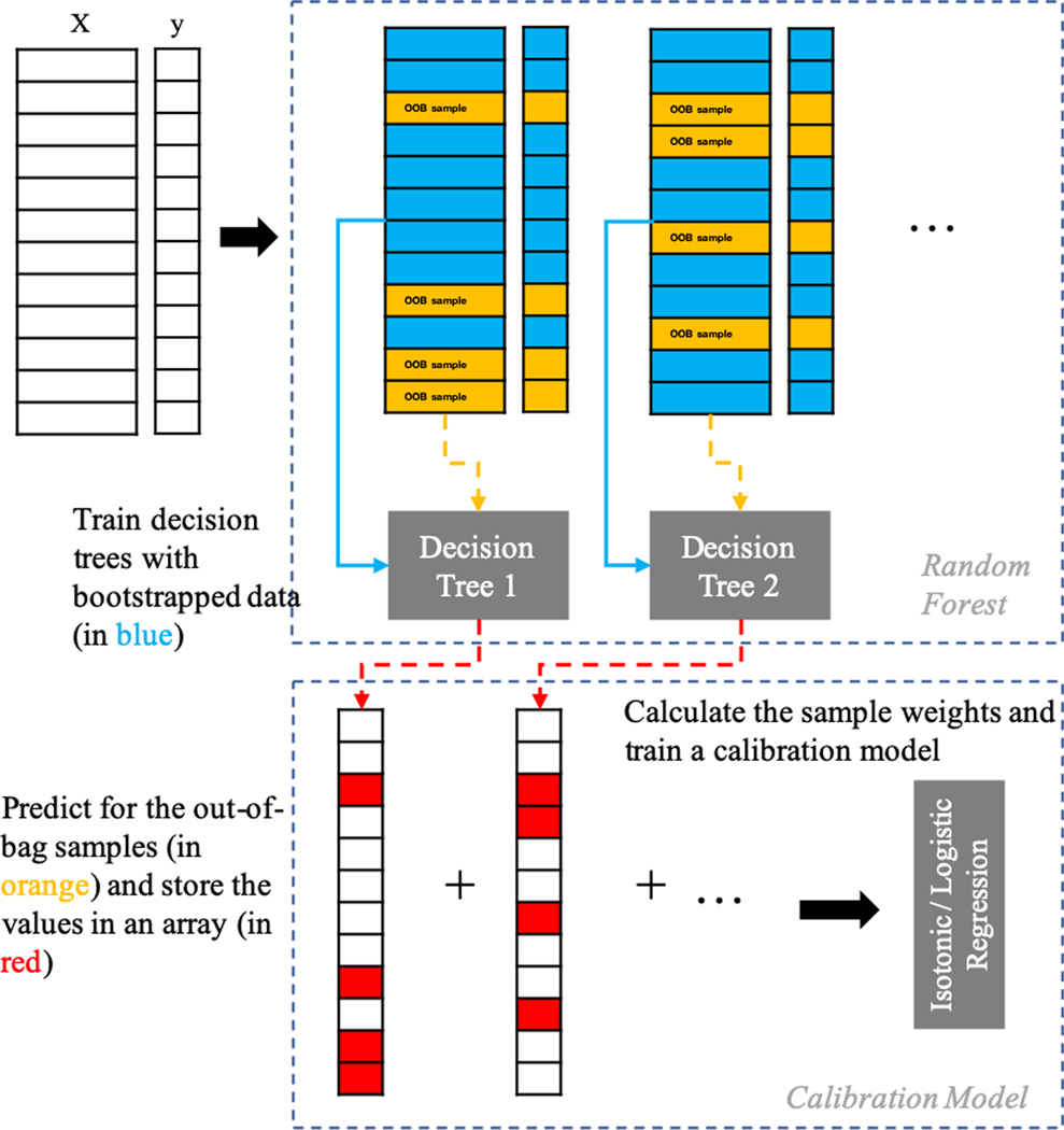
CaliForest mitigates the noise in the OOB predictions by utilizing each individual OOB sample prediction from each tree. The key observation is to calculate the variance of the individual tree predictions to estimate the certainty of the OOB prediction. Conceptually, if all the OOB sample predictions for a single sample across the various trees are similar, then it is more likely the other trees will produce a similar result. However, if all the OOB sample predictions have a large range, then we should be less certain about that particular sample. The calibration model can then leverage this information in the form of sample weights to learn a robust calibration function. The process is illustrated in Figure 1.
Figure 1:
An illustration of the CaliForest process. The key observation is the use of the individual predictions on the out-of-bag sample to calculate a weight associated with each sample.
3.1. CaliForest Sample Weights
For each sample, the estimated prediction from the random forest can be decomposed into two parts, the OOB prediction and the non-OOB prediction.
| (1) |
| (2) |
The OOB prediction can be obtained directly from the random forest, while the non-OOB prediction is unobserved. Thus, we can approximate the estimated sample prediction to be centered around the OOB prediction with some noise. Under the assumption that there will be sufficient trees, the noise will follow a normal distribution centered around 0 with unknown variance, :
| (3) |
Since each sample will belong to a varying number of OOB samples (i.e., 0 to total number of trees), we estimate the variance of the noise using the Bayesian update associated with an Inverse Gamma conjugate prior. Thus, if the ith sample belongs to a large number of OOB samples and has a low sample variance, the estimate should be close to the corresponding sample variance, . If the ith sample is not selected for any OOB samples, then it should take the maximum possible variance for a bounded random variable between 0 and 1, which is 0.25. Note that the prior variance is thereby assumed to be 0.25 (= β0/α0), or the maximum possible variance. Therefore, the variance is estimated using the following updates:
| (4) |
| (5) |
| (6) |
Each sample weight is then inversely proportional to the variance,
| (7) |
The idea is that if the variance is small, then the estimated prediction from the random forest, will be close to the OOB prediction . Therefore, the calibration model should trust this sample more. However, if the variance is large, then the estimated prediction may be quite different from the OOB prediction, and thus should be discounted in the learned calibration. The sample weights can then be passed with the OOB predictions to either the isotonic regression or logistic regression model.
3.2. Python Package
We developed califorest, an open-source Python package, to enable widespread usage of CaliForest. califorest builds on scikit-learn, a standard Python module that integrates a wide range of state-of-the-art machine learning algorithms [20]. By following the scikit-learn coding convention, a practitioner can easily deploy CaliForest to achieve both good discrimination and calibration. The package is published on the Python Package Index (PyPI), a standard Python software repository. Therefore, it can be installed using the standard “pip install califorest” command. Additionally, the code is also openly available on GitHub at https://github.com/yubin-park/califorest under the permissive MIT license. This will enable continuous and collaborative development.
The usage of the califorest package is identical to using any machine learning module from scikit-learn. First, the package is imported into the Python environment. The CaliForest algorithm is then applied by creating an instance of the CaliForest class. The CaliForest model is then trained by calling the fit function with two arguments, the input data array (or features) and the array of labels. Since CaliForest is a supervised estimator, it also provides the predict function to predict the class label for new data. Thus, the usage is as follows:
| 1 from c a l i f o r e s t import C a l i F o r e s t |
| 2 |
| 3 model = C a l i F o r e s t ( ) |
| 4 model . f i t ( X_train , y _ t r a i n ) |
| 5 model . p r e d i c t ( X_test ) |
Therefore, CaliForest can be easily exchanged in existing software appplications that already utilize the RandomForest classifier from scikit-learn.
The califorest package also contains implementations for five of the six calibration metrics (except Brier score) described in Table 1. Note that scikit-learn already has an implementation for the Brier score. The calibration metrics also follow the evaluation metric convention introduced in scikit-learn. In particular, each metric has its own function and the two arguments to be passed into the function are the true labels and the estimated risk. Thus, the usage for the scaled Brier score is as follows:
| 1 from c a l i f o r e s t import me t r i c s |
| 2 |
| 3 me t r i c s . s c a l e d _ b r i e r _ s c o r e ( y_t rue , y_pred ) |
4. EXPERIMENTAL RESULTS
We will illustrate the benefits of CaliForest on several binary prediction tasks using real-world electronic health records.
4.1. Data
We used MIMIC-III, a publicly-available, de-identified dataset that contains information about intensive care unit (ICU) patients from the Beth Israel Deaconess Medical Center [16]. We focused on two varieties of two common risk prediction tasks, mortality and long length-of-stay (LOS). These prediction tasks were chosen since they have been highlighted as benchmark tasks in several existing works [9, 22, 29]. Moreover, random forests have been shown to achieve great performance on these tasks [7, 18]. The four binary prediction tasks are:
In-ICU mortality: Predict whether the patient dies during the ICU stay after ICU admission.
In-hospital mortality: Predict whether the patient dies during the hospital stay after ICU admission.
Length-of-stay > 3 days: Predict whether the patient will stay in the ICU longer than 3 days.
Length-of-stay > 7 days: Predict whether the patient will stay in the ICU longer than 7 days.
Table 2 summarizes the statistics for the four prediction tasks.
Table 2:
The summary statistics for the four prediction tasks.
| Task | Samples | Features | Prevalence |
|---|---|---|---|
| In-hospital Mortality | 23,937 | 7,488 | 10.52% |
| In-ICU Mortality | 23,937 | 7,488 | 7.09% |
| Length-of-stay > 3 | 23,937 | 7,488 | 42.96% |
| Length-of-stay > 7 | 23,937 | 7,488 | 7.70% |
We used MIMIC-Extract [29], an open-source pipeline, to construct the data cohort and the four binary prediction tasks. We use the default cohort construction, which focuses on the patient’s first ICU visit and requires patients to be over 15 years old and have at least 30 hours of data present. Only the first 24 hours of a patient’s data is considered. Time-varying labs and vitals are grouped together into hourly summary statistics, and static demographic features are one-hot encoded. All the values are mean-centered and scaled to have a unit variance. Missing data are imputed using the scheme outlined in [7]. For details of the data standardization and aggregation, see [29].
4.2. Baseline Models and Evaluation Setup
CaliForest is compared with calibrated random forest and the uncalibrated random forest. For both CaliForest and random forest, both the Platt scaling and isotonic regression function are used as calibration models. Thus, we evaluated five different models:
CaliForest with isotonic regression (CF-Iso): Our model with the calibration model using the isotonic regression function trained on the sample weighted out-of-bag samples shown in Figure 1.
CaliForest with Platt scaling (CF-Logit): Similar to the CF-Iso model above except the calibration model is the Platt scaling function.
Random forest calibration with isotonic regression (RC-Iso): The random forest model trained on 70% of the training data and the isotonic regression function is then learned on the 30% calibration set.
Random forest calibration with Platt scaling (RC-Logit): Similar to the RF-IOS model above except the sigmoid function is learned on the 30% calibration set.
Random Forest with no calibration (RF-NoCal): The standard scikit-learn random forest model learned on the entire training set without any calibration model applied.
We did not include the calibrated random forests proposed by Boström [6] as our experiments did not show any difference between this model and the Random Forest with isotonic regression.
Each model was evaluated using the same 10 Monte Carlo cross-validation samples, each with a 70–30 train-test split. We tuned the maximum depth of the decision tree and the number of estimators in the random forest model using the out-of-bag samples. It is important to note that since both isotonic regression and Platt scaling perform a monotonic transformation of the random forest model predictions, the sample rankings are predominantly preserved and thus their predictive performance (as measured by AUROC) is unlikely to change substantially. We compared each model based on the six commonly published calibration metrics (summarized in Table 1) evaluated on the test set. For the scaled Brier score, Hosmer-Lemeshow p-value, and Spiegelhalter p-value metrics, the higher the number (closer to 1), the better calibrated the model is. For the Brier score, reliability-in-the-small, and reliability-in-the-large metrics, the lower the number (closer to 0), the better calibrated the model is.
4.3. Mortality Prediction
4.3.1. In-hospital mortality.
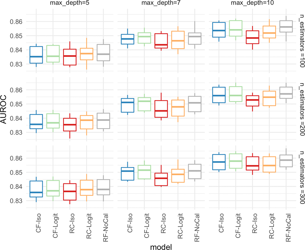
First, we present an in-depth case study on the in-hospital mortality prediction task. Figure 2 presents the AUROC (predictive performance) for the five different models over the two hyperparameters, decision tree depth and the number of estimators. The predictive performance improves as the individual trees are grown deeper (last column of plots with depth=10) and there are more trees (last row of plots with n_estimators=300). It can also be observed from the figure that both RC-Iso and RC-Logit have a slightly worse performance with deeper trees (depth ≥ 7) due to the difference in training data. Since RC-Iso and RC-Logit are only trained on 70% of the data, the individual trees do not generalize as well.
Figure 2:
[In-hospital Mortality] AUROC over different hyperparameters with maximum tree depth = [5,7,10] (column) and number of estimators = [100,200,300] (row).
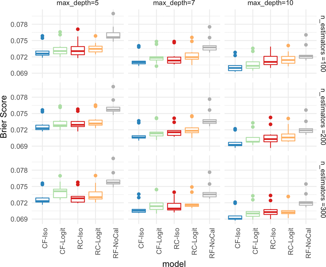
To better understand the impact of the hyperparameters on the calibration performance, Figure 3 illustrates the Brier score for each of the five different models. As the trees become deeper and there are more trees, the Brier score improves which indicates the overall calibration of the models is better. The figure also illustrates the importance of learning a calibration function using a calibration set, as the calibrated models all have lower Brier scores than RF-NoCal. A closer comparison of the standard calibration approach (RC-Iso, RC-Logit) with the non-calibrated version (RF-NoCal) on Figures 2 and 3 illustrate the well-known trade-off between discrimination and calibration for limited samples. However, CaliForest can achieve both comparable discriminative performance with the non-calibrated version and have the lowest Brier score amongst all the models. This illustrates the power of utilizing the sample weights to estimate a better calibration function.
Figure 3:
[In-hospital Mortality] Brier Score over different hyperparameters with maximum tree depth = [5,7,10] (column) and number of estimators = [100,200,300] (row).
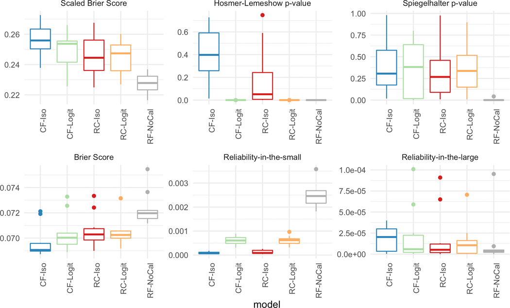
Figure 4 plots the performance of the five models using depth = 10 and 300 trees across the six different metrics. For the top row (i.e., scaled Brier score, Hosmer-Lemeshow p-value, and Spiegelhalter p-value), a higher value signifies better calibration while for the lower row (i.e., Brier score, reliability-in-the-small, and reliability-in-the-large), a lower value indicates a better calibration model. Except for the reliability-in-the-large, across all other five calibration metrics, CF-Iso outperforms the other 4 models. In fact, the performance differences for the reliability-in-the-large are not statistically significant given the range of the values (≈ 1e − 5). As can be seen, the calibrated models generally outperform the standard random forest model across all the metrics.
Figure 4:
[In-hospital Mortality] Calibration metrics for the five models with depth = 10 and number of estimators = 300.
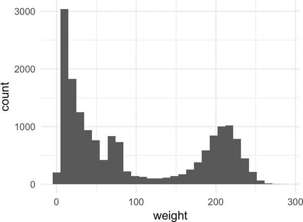
Figure 5 explores the relationship between the sample weights, the OOB prediction, and the isotonic fit. In Figure 5a, we observe that about a half of the samples have small weights (weight ≤ 50), while another half have a large weight (weight ≥ 200). This indicates that there are two groups of OOB predictions: reliable and unreliable predictions. The plot (5a) also illustrates the limitation of naively using the OOB prediction itself to learn the calibration function, as a significant portion of the OOB samples will be noisy.
Figure 5:
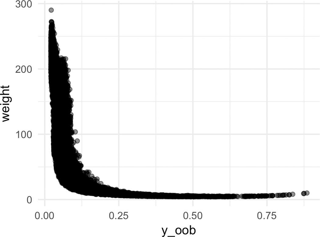
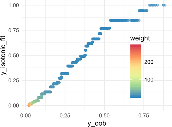
[In-hospital Mortality] Sample weight characteristics for CF-Iso using depth = 10 and number of estimators = 300.
Figure 5b plots the relationship between the OOB prediction and the sample weights. The majority of the small weights (weight ≤ 50) are associated with non-zero estimated risk This suggests that a handful of trees are certain these samples should be positive and are pushing up the OOB prediction scores, but in fact there is a large variance in the estimated predictions themselves. Thus, the learned calibration function can potentially pull these values down. This is further substantiated in Figure 5c which showcases that the piece-wise step function isotonic regression has a linear relationship for the lower values before flattening out towards the larger OOB predictions.
4.3.2. In-ICU mortality.
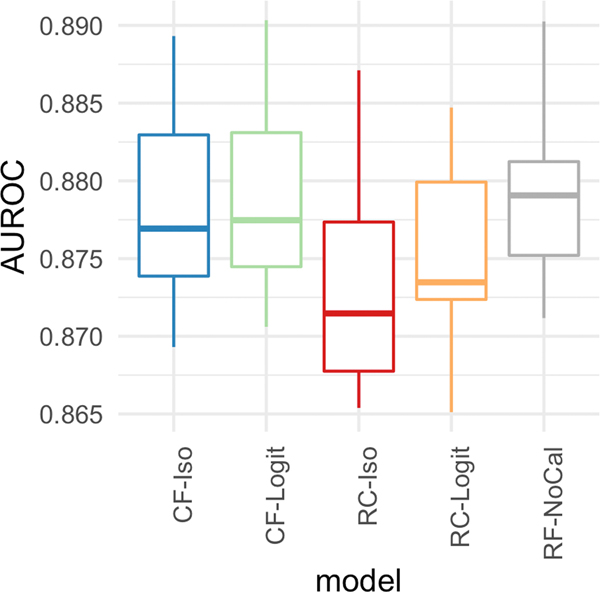
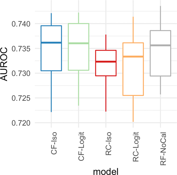
Next, we evaluate the calibration of the various random forest models on the In-ICU mortality task. The best performance is achieved with deeper trees (depth = 10) and more trees (number of estimators=300). In addition, the discrimination is similar between CF-Iso, CF-Logit, RF-NoCal, while RC-ISo and RC-Logit have a slightly lower performance due to setting aside 30% for a calibration set as shown in Figure 6a.
Figure 6:
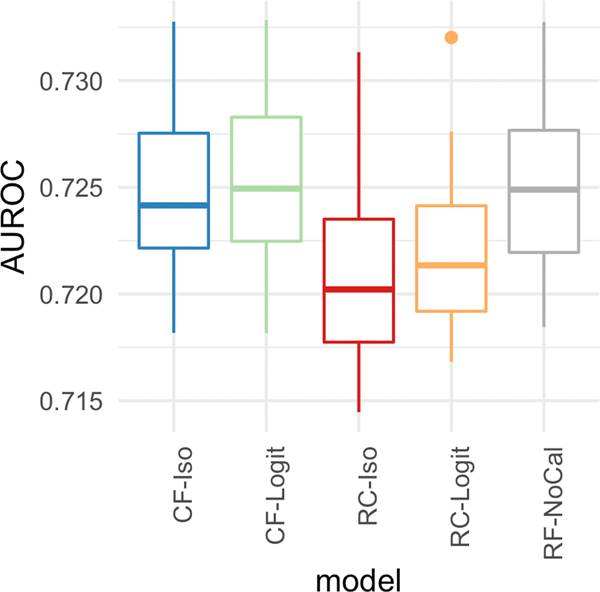
AUROCs for the best hyperparameter for the ICU-Mortality, 3 and 7 Day LOS prediction tasks.
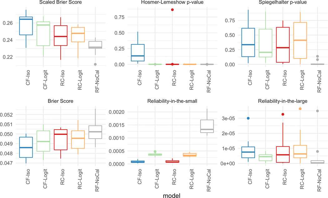
Figure 7 plots the performance of the five models on the six different calibration metrics. Similar to the in-hospital mortality task, CF-Iso generally achieves the best calibration. The exceptions where CF-Iso is not noticeably better are according to the Spiegelhalter p-value and the reliability-in-the-large. However, the variance of the Spiegelhalter p-value across the 10 different cross-validation samples for CF-Iso is smaller than RC-ISO and RC-Logit. Also, the performance differences of the reliability-in-the-large are not statistically significant given the range of the values. Thus, Figure 7 suggests that CF-Iso is overall the best-calibrated model. The figure also showcases that calibrating the random forest model generally seems to help the overall-calibration compared to the non-calibrated case (RF-NoCal).
Figure 7:
[ICU Mortality] Calibration metrics for the five models with depth = 10 and number of estimators = 30.
4.4. Length-of-stay Prediction
4.4.1. Length-of-stay > 3 days.
Next, we evaluate the calibration of the various random forest models on predicting whether the patient will stay in the ICU longer than 3 days. The best performance is achieved with deeper trees (depth = 10) and more trees (number of estimators=300). In addition, the discrimination is similar between CF-Iso, CF-Logit, RF-NoCal, while RC-ISo and RC-Logit have a slightly lower performance due to setting aside 30% for a calibration set as shown in Figure 6b.
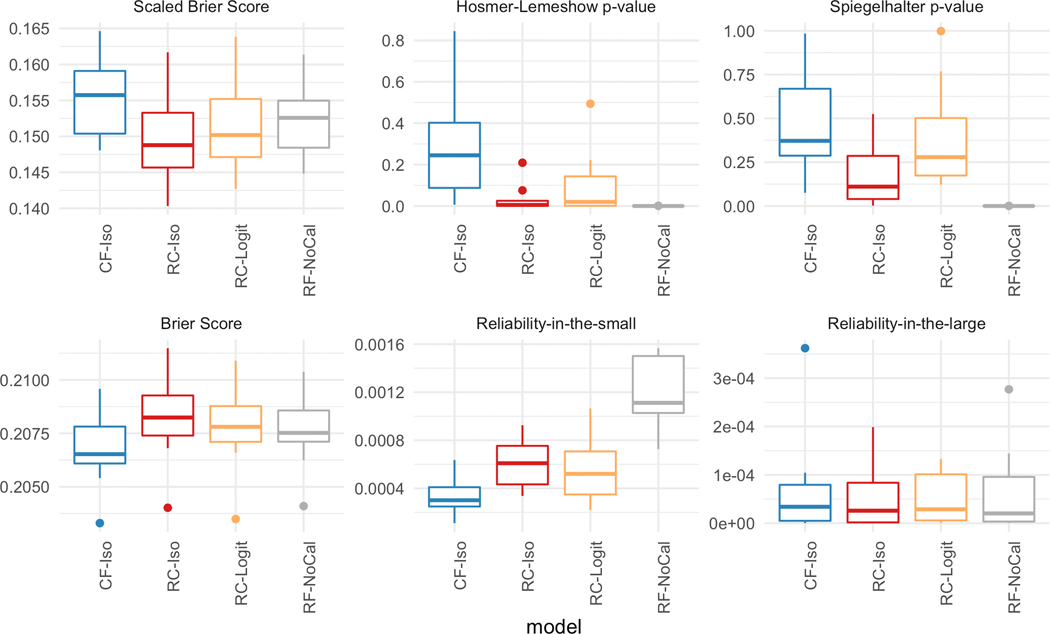
Figure 8 plots the calibration performance on the task of predicting Length-of-stay > 3 days. Similar to the previous two tasks, CF-Iso generally achieves the best calibration. Unlike the previous mortality prediction tasks, there is no clear benefit of setting aside a calibration set to improve the calibration. For scaled Brier score, Brier score, and the Hosmer-Lemeshow p-value, there is no noticeable improvement in Figure 8. This coupled with the decrease in discriminative performance (shown in Figure 6b) illustrates the limitation of the separate calibration set.
Figure 8:
[3 Day LOS] Calibration metrics for the five models with depth = 10 and number of estimators = 300. The calibration performance of CF-Logit is not displayed due to its unstable performance.
4.4.2. Length-of-stay > 7 days.
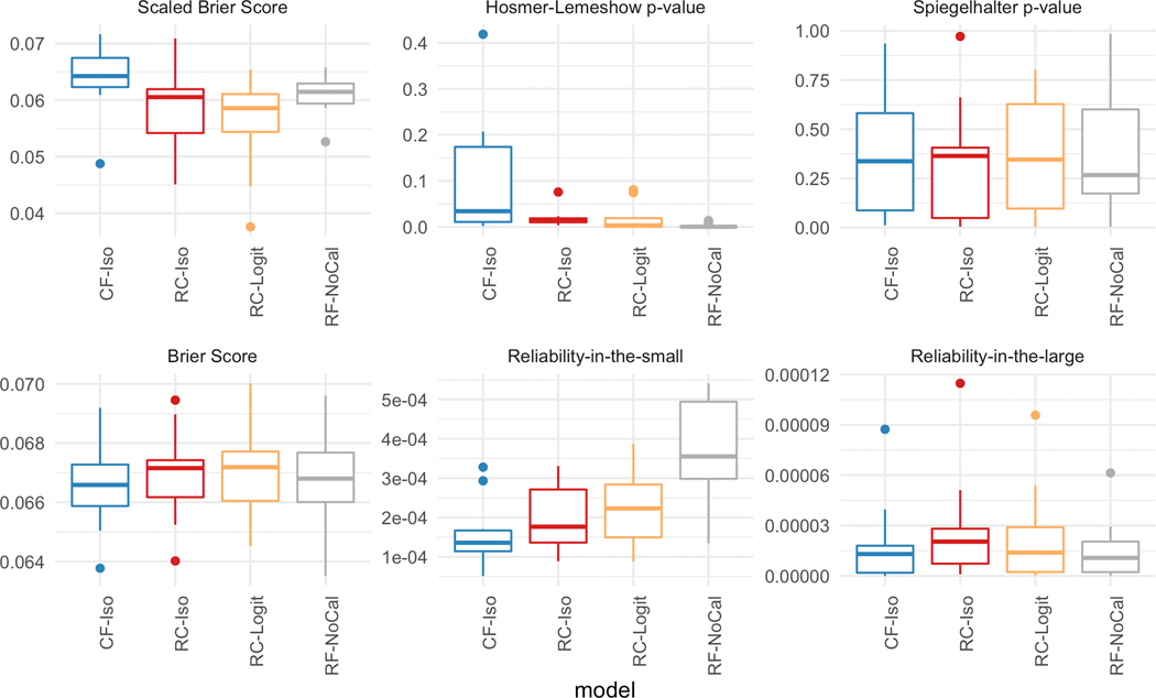
Last, we evaluate the calibration of the various random forest models on predicting whether the patient will stay in the ICU longer than 7 days. The best performance is achieved with shallower trees (depth = 5) and more trees (number of estimators=300). We observe that similar to the previous three tasks, the discrimination is similar between CF-Iso, CF-Logit, RF-NoCal, while RC-Iso and RC-Logit have a slightly lower performance due to setting aside 30% for a calibration set as shown in Figure 6c. Figure 9 plots the calibration performance of the models on 7 day LOS. As was the trend for the other three tasks, CF-Iso outperforms the other models.
Figure 9:
[7 Day LOS] Calibration metrics for the five models with depth = 5 and number of estimators = 300. The calibration performance of CF-Logit is not displayed due to its unstable performance.
5. DISCUSSIONS
We introduced CaliForest, a calibrated random forest model, to improve the calibration of random forest without sacrificing the discrimination ability of the model. CaliForest utilizes the OOB samples to learn the calibration model. However, instead of blindly trusting the OOB predictions, CaliForest considers the variance of the OOB prediction to determine the importance of the sample. By accounting for the uncertainty in the non-OOB predictions, the learned calibration function can substantially improve the calibration of the models.
We demonstrated CaliForest on four binary prediction tasks using MIMIC-III data. Our empirical results illustrate the benefits of utilizing the OOB predictions to estimate the sample weights and predictions, which are both then used to learn the calibration function. The results across the four tasks suggest that using isotonic regression as the calibration method maintains the same discrimination of the standard random forest, while improving the calibration of the model measured on a variety of calibration metrics.
An interesting observation drawn from the experiments is that CaliForest using the Platt scaling function as a calibration model did not always yield improved calibration. One hypothesis is the sigmoid function was not an appropriate calibration function for these tasks, as the risk predictions may be biased. Another hypothesis is that the sample weights need to be tailored for the sigmoid function separately. Further exploration of the sample weights for the Platt scaling function is left for future work. In addition, CaliForest can be generalized to encompass other calibration functions such as the adaptive calibration procedure introduced in [14] or the Venn-Abers predictors [15].
CaliForest is published on the standard Python software repository under the califorest package and the code will be openly available on Github (URL: https://github.com/yubin-park/califorest). The package enables software developers to easily exchange existing software deployments that utilize the random forest classifier from scikit-learn with CaliForest for improved calibration. Moreover, the release of the califorest package also enables calibration to be examined more thoroughly, with the calibration metrics described in Table 1 already implemented.
ACKNOWLEDGMENTS
This work was supported by National Institute of Health award 1K01LM012924–01.
Permission to make digital or hard copies of part or all of this work for personal or classroom use is granted without fee provided that copies are not made or distributed for profit or commercial advantage and that copies bear this notice and the full citation on the first page. Copyrights for third-party components of this work must be honored. For all other uses, contact the owner/author(s).
Contributor Information
Yubin Park, Emory University Bonsai Research, LLC.
Joyce C. Ho, Emory University
REFERENCES
- [1].Alba Ana Carolina, Agoritsas Thomas, Walsh Michael, Hanna Steven, Iorio Alfonso, Devereaux PJ, McGinn Thomas, and Guyatt Gordon. 2017. Discrimination and Calibration of Clinical Prediction Models: Users’ Guides to the Medical Literature. JAMA 318, 14 (2017), 1377–1384. [DOI] [PubMed] [Google Scholar]
- [2].Anderson Ariana E, Kerr Wesley T, Thames April, Li Tong, Xiao Jiayang, and Cohen Mark S. 2016. Electronic health record phenotyping improves detection and screening of type 2 diabetes in the general United States population: A cross-sectional, unselected, retrospective study. Journal of Biomedical Informatics 60 (2016), 162–168. [DOI] [PMC free article] [PubMed] [Google Scholar]
- [3].Ayer Turgay, Alagoz Oguzhan, Chhatwal Jagpreet, Shavlik Jude W, Kahn Charles E, and Burnside Elizabeth S. 2010. Breast cancer risk estimation with artificial neural networks revisited: discrimination and calibration. Cancer 116, 14 (2010), 3310–3321. [DOI] [PMC free article] [PubMed] [Google Scholar]
- [4].Badger Jonathan, Eric LaRose John Mayer, Bashiri Fereshteh, Page David, and Peissig Peggy. 2019. Machine Learning for Phenotyping Opioid Overdose Events. Journal of Biomedical Informatics 94 (2019), 103185. [DOI] [PMC free article] [PubMed] [Google Scholar]
- [5].Bates David W, Saria Suchi, Ohno-Machado Lucila, Shah Anand, and Escobar Gabriel. 2014. Big data in health care: using analytics to identify and manage high-risk and high-cost patients. Health Affairs 33, 7 (2014), 1123–1131. [DOI] [PubMed] [Google Scholar]
- [6].Boström Henrik. 2008. Calibrating Random Forests. 2008 Seventh International Conference on Machine Learning and Applications (2008), 121–126. [Google Scholar]
- [7].Che Zhengping, Purushotham Sanjay, Cho Kyunghyun, Sontag David, and Liu Yan. 2018. Recurrent Neural Networks for Multivariate Time Series with Missing Values. Scientific Reports 8, 1 (2018), 6085. [DOI] [PMC free article] [PubMed] [Google Scholar]
- [8].Domingos Pedro and Pazzani Michael. 1997. On the Optimality of the Simple Bayesian Classifier under Zero-One Loss. Machine Learning 29, 2/3 (1997), 103–130. [Google Scholar]
- [9].Harutyunyan Hrayr, Khachatrian Hrant, David C Kale Greg Ver Steeg, and Galstyan Aram. 2019. Multitask learning and benchmarking with clinical time series data. Scientific Data 6, 1 (2019), 96. [DOI] [PMC free article] [PubMed] [Google Scholar]
- [10].Hooks Mary A. 2010. Breast Cancer: Risk Assessment and Prevention. Southern Medical Journal 103, 4 (2010), 333–338. [DOI] [PubMed] [Google Scholar]
- [11].Hosmer DW, Hosmer T, Cessie S Le, and Lemeshow S. 1997. A comparison of goodness-of-fit tests for the logistic regression model. Statistics in Medicine 16, 9 (1997), 965–980. [DOI] [PubMed] [Google Scholar]
- [12].Hu Zhongkai, Hao Shiying, Jin Bo, Young Shin Andrew, Zhu Chunqing, Huang Min, Wang Yue, Zheng Le, Dai Dorothy, Culver Devore S, Alfreds Shaun T, Rogow Todd, Stearns Frank, Sylvester Karl G, Widen Eric, and Ling Xuefeng. 2015. Online prediction of health care utilization in the next six months based on electronic health record information: A cohort and validation study. Journal of Medical Internet Research 17, 9 (2015), e219. [DOI] [PMC free article] [PubMed] [Google Scholar]
- [13].Jiang Xiaoqian, Menon Aditya, Wang Shuang, Kim Jihoon, and Lucila Ohno-Machado. 2012. Doubly Optimized Calibrated Support Vector Machine (DOCSVM): An Algorithm for Joint Optimization of Discrimination and Calibration. PLoS ONE 7, 11 (2012), e48823. [DOI] [PMC free article] [PubMed] [Google Scholar]
- [14].Jiang Xiaoqian, Osl Melanie, Kim Jihoon, and Lucila Ohno-Machado. 2012. Calibrating predictive model estimates to support personalized medicine. Journal of the American Medical Informatics Association 19, 2 (2012), 263–274. [DOI] [PMC free article] [PubMed] [Google Scholar]
- [15].Johansson Ulf, Löfström Tuwe, and Boström Henrik. 2019. Calibrating Probability Estimation Trees using Venn-Abers Predictors. In SDM. 28–36. [Google Scholar]
- [16].Johnson Alistair E W, Pollard Tom J, Shen Lu, Lehman Li-wei H, Feng Mengling, Ghassemi Mohammad, Moody Benjamin, Szolovits Peter, Celi Leo Anthony, and Mark Roger G. 2016. MIMIC-III, a freely accessible critical care database. Scientific Data 3 (2016), 160035. [DOI] [PMC free article] [PubMed] [Google Scholar]
- [17].Khalilia Mohammed, Chakraborty Sounak, and Popescu Mihail. 2011. Predicting disease risks from highly imbalanced data using random forest. BMC Medical Informatics and Decision Making 11, 1 (2011), 51. [DOI] [PMC free article] [PubMed] [Google Scholar]
- [18].Nestor Bret, Matthew McDermott Willie Boag, Berner Gabriela, Naumann Tristan, Michael C Hughes Anna Goldenberg, and Ghassemi Marzyeh. 2019. Feature robustness in non-stationary health records: caveats to deployable model performance in common clinical machine learning tasks. arXiv preprint arXiv:1908.00690 (2019). [Google Scholar]
- [19].Obermeyer Ziad and Emanuel Ezekiel J. 2016. Predicting the future - Big data, machine learning, and clinical medicine. The New England Journal of Medicine 375, 13 (2016), 1216–1219. [DOI] [PMC free article] [PubMed] [Google Scholar]
- [20].Pedregosa Fabian, Varoquaux Gaël, Gramfort Alexandre, Michel Vincent, Thirion Bertrand, Grisel Olivier, Blondel Mathieu, Prettenhofer Peter, Weiss Ron, Dubourg Vincent, et al. 2011. Scikit-learn: Machine learning in Python. Journal of Machine Learning Research 12, Oct (2011), 2825–2830. [Google Scholar]
- [21].Platt John. 1999. Probabilistic outputs for support vector machines and comparisons to regularized likelihood methods. Advances in large margin classifiers 10, 3 (1999), 61–74. [Google Scholar]
- [22].Purushotham Sanjay, Meng Chuizheng, Che Zhengping, and Liu Yan. 2018. Bench-marking deep learning models on large healthcare datasets. Journal of Biomedical Informatics 83 (2018), 112–134. [DOI] [PubMed] [Google Scholar]
- [23].Rufibach Kaspar. 2010. Use of Brier score to assess binary predictions. Journal of Clinical Epidemiology 63, 8 (2010), 938–939. [DOI] [PubMed] [Google Scholar]
- [24].Spiegelhalter DJ. 1986. Probabilistic prediction in patient management and clinical trials. Statistics in Medicine 5, 5 (1986), 421–433. [DOI] [PubMed] [Google Scholar]
- [25].Steyerberg Ewout W et al. 2009. Clinical prediction models. Vol. 381. Springer. [Google Scholar]
- [26].Steyerberg Ewout W, Vickers Andrew J, Cook Nancy R, Gerds Thomas, Gonen Mithat, Obuchowski Nancy, Pencina Michael J, and Kattan Michael W. 2010. Assessing the performance of prediction models: a framework for some traditional and novel measures. Epidemiology 21, 1 (2010), 128–138. [DOI] [PMC free article] [PubMed] [Google Scholar]
- [27].Sun Jimeng, Candace D McNaughton Ping Zhang, Perer Adam, Gkoulalas-Divanis Aris, Denny Joshua C, Kirby Jacqueline, Lasko Thomas, Saip Alexander, and Malin Bradley A. 2013. Predicting changes in hypertension control using electronic health records from a chronic disease management program. Journal of the American Medical Informatics Association 21, 2 (2013). [DOI] [PMC free article] [PubMed] [Google Scholar]
- [28].Walsh Colin G., Sharman Kavya, and Hripcsak George. 2017. Beyond discrimination: A comparison of calibration methods and clinical usefulness of predictive models of readmission risk. Journal of Biomedical Informatics 76 (2017), 9–18. [DOI] [PMC free article] [PubMed] [Google Scholar]
- [29].Wang Shirly, Matthew McDermott Geeticka Chauhan, Michael C Hughes Tristan Naumann, and Ghassemi Marzyeh. 2019. Mimic-extract: A data extraction, preprocessing, and representation pipeline for mimic-iii. arXiv preprint arXiv:1907.08322 (2019). [Google Scholar]
- [30].Yates J Frank. 1982. External correspondence: Decompositions of the mean probability score. Organizational Behavior and Human Performance 30, 1 (1982), 132–156. [Google Scholar]
- [31].Zadrozny Bianca and Elkan Charles. 2001. Obtaining calibrated probability estimates from decision trees and naive Bayesian classifiers. In ICML, Vol. 1. 609–616. [Google Scholar]
- [32].Zhao Juan, Feng QiPing, Wu Patrick, Lupu Roxana A., Wilke Russell A., Wells Quinn S., Denny Joshua C., and Wei Wei-Qi. 2019. Learning from Longitudinal Data in Electronic Health Record and Genetic Data to Improve Cardiovascular Event Prediction. Scientific Reports 9, 1 (2019), 717. [DOI] [PMC free article] [PubMed] [Google Scholar]
- [33].Zheng Tao, Xie Wei, Xu Liling, He Xiaoying, Zhang Ya, You Mingrong, Yang Gong, and Chen You. 2017. A machine learning-based framework to identify type 2 diabetes through electronic health records. International Journal of Medical Informatics 97, JAMA 310 9 2013 (2017), 120–127. [DOI] [PMC free article] [PubMed] [Google Scholar]


