An artificial neural network−pharmacokinetic model and its interpretation using Shapley additive explanations

Abstract

We developed a method to apply artificial neural networks (ANNs) for predicting time‐series pharmacokinetics (PKs), and an interpretable the ANN‐PK model, which can explain the evidence of prediction by applying Shapley additive explanations (SHAP). A previous population PK (PopPK) model of cyclosporin A was used as the comparison model. The patients’ data were used for the ANN‐PK model input, and the output by ANN was the clearance (CL). The estimated CL value from the ANN were substituted into the one‐compartment with one‐order absorption model, the concentrations were calculated, and the parameters of ANN were updated by the back‐propagation method. Kernel SHAP was applied to the trained model and the SHAP value of each input was calculated. The root mean squared error for the PopPK model and the ANN‐PK model were 41.1 and 31.0 ng/ml, respectively. The goodness of fit plots for the ANN‐PK model represented more convergence to y = x compared with that for the PopPK model, with good model performance for the ANN‐PK model. The most influential factors on CL output were age and body weight from the evaluation using Kernel SHAP, and these factors were incorporated into the PopPK model as the significant covariates of CL. The ANN‐PK model could handle time‐series data and showed higher prediction accuracy then the conventional PopPK model, and the scientific validity for the model could be evaluated by applying SHAP.

Study Highlights.

• WHAT IS THE CURRENT KNOWLEDGE ON THE TOPIC?

A black‐box property of an artificial neural network (ANN) decreases the scientific confidence of the model, and making it difficult to utilize the ANN in the medical field. Moreover, difficulty in handling the time‐series data is a significant problem for applying the ANN for pharmacometrics study.

• WHAT QUESTION DID THIS STUDY ADDRESS?

How can we apply the ANN for predicting the time‐series pharmacokinetics (PKs) , and confirm the scientific validity of the ANN model?

• WHAT DOES THIS STUDY ADD TO OUR KNOWLEDGE?

Using the ANN in combination with a conventional compartment (ANN‐PK) model enabled to handle the time‐series PK data, and the predicting performance of the model was higher than that of the population PK model. Furthermore, we could evaluate the scientific validity of the ANN model by applying the Shapley additive explanations.

• HOW MIGHT THIS CHANGE DRUG DISCOVERY, DEVELOPMENT, AND/OR THERAPEUTICS?

We expect that our study will contribute to develop the interpretable ANN model, which can predict the time‐series PKs, drug efficacies, and side effects with high prediction performance.

INTRODUCTION

The handling of big data and complex mathematical models has become possible with developments in computer technology and data sciences, such as artificial intelligence (AI) and machine learning. ¹ In the medical field, the focus has been on the application of AI to diagnosis using medical image data, drug discovery, and drug repositioning. ² , ³ , ⁴ , ⁵ Some studies have tried to apply AI and machine learning to pharmacometrics. ⁶ , ⁷ , ⁸ , ⁹ For example, Yamashita et al. automated covariate selection in pharmacometrics model building by applying gene expression programing, making it possible to build a significantly better fitting model than a previous one. ⁶ Some researchers have applied tree algorithms and artificial neural networks (ANNs) to pharmacometrics. ⁹ , ¹⁰

The trigger of the current AI boom is deep learning, a machine‐learning method using a deep neural network (DNN) in which the machine‐learning model mimics the neurotransmitter system. ¹¹ DNN, a model based on ANN, has multiple (deep) hidden layers. Both ANN and DNN consist of three types of layers: input layer, hidden layers, and output layer. ¹² Each layer has multiple units called neurons, and the sum of the weighted value of each unit is propagated to the next layer. ANN and DNN can learn the features of data by themselves, thus improving the analytical accuracy of data from which it is difficult to extract features, such as image data. ¹³

Application of ANN and DNN is expected to improve the accuracy of predicting pharmacokinetics (PKs), clinical efficacies, and side effects by identifying features of data that have not been discovered in previous empirical modeling. However, there are two significant problems in utilizing these machine‐learning models in pharmacometrics. First, the progress from input to output becomes a black‐box by using ANN or DNN, and the interpretability of the model markedly decreases. ¹⁴ , ¹⁵ , ¹⁶ Even if the developed model has great accuracy and performance, it may be difficult to use it in the drug development or medical settings because developers and physicians cannot judge if the model is scientifically appropriate. The second problem is that it is difficult for ANN and DNN to handle time‐series data. The principle of pharmacometrics is evaluating time‐series variations in PKs and pharmacodynamics. There are some techniques for handling time‐series data with ANN and DNN, such as recurrent neural networks, but as the complexity of the models increase, their interpretability decreases. ¹⁷ Yamamura et al. have reported a study which applied ANN to predict drug blood concentration, but the sampling timing was fixed and their model could only predict drug concentrations for limited timing. ⁹

The interpretability of a model decreases in exchange for an increase in its accuracy. This is a problem not only for deep learning, but also for ensemble learning and gradient boosting methods, which have become popular in recent years. ¹⁸ , ¹⁹ , ²⁰ The rationale for the results obtained from simpler decision tree models can be easily explained, but accuracy becomes a trade‐off for simplicity. ²¹ Ensample learning enables the construction of models with better accuracy and handles more complex data, but these models are usually more complex than traditional machine‐learning models. ²² , ²³ Therefore, Shapley additive explanations (SHAP) have been suggested to calculate the contribution of each feature (input) to the output. ¹⁹ SHAP is an extension of a Shapley value in cooperative game theory as a method for calculating the contribution of each feature in machine learning. SHAP values are calculated by determining the difference between the predicted values with and without the addition of each feature (i.e., the effect of adding each feature) for all combinations, and taking the average. It thus becomes possible to understand which features have a significant influence on the output (prediction) and whether the influence is positive or negative by calculating the SHAP values.

The aims of this study were (1) to develop and evaluate a method to apply ANN for predicting time‐series PKs, and (2) to develop an interpretable AI model which can explain the evidence of prediction by applying SHAP.

METHODS

Comparison model (population pharmacokinetic model)

This study was conducted with the approval of the ethics committee of Nihon University (School of Pharmacy, approval number: 20‐012). A previous population PK (PopPK) model of cyclosporin A was used as the comparison model. ²⁴ The same data as the previous study were used for the present analysis, and the data used were from 36 patients with 89 drug blood concentrations. Details of the comparison PopPK model are shown in Table S1. The final PopPK model in the previous study was a one‐compartment with a one‐order absorption model, and the influence of age and of body weight of the patients were incorporated into the model as significant covariates for clearance.

Artificial neural network pharmacokinetic model

The basic structure of the ANN‐PK model is presented in Figure 1. The clinical data and background of patients were used for the model input, and the output by ANN was the clearance (CL). The estimated CL value from the ANN, the previously reported values of a volume of distribution, and an absorption rate constant were substituted into the one‐compartment with one‐order absorption model, and predictions of drug concentrations were calculated. Differences between the predictions and observed values were calculated, and the weights in the ANN were updated by the back‐propagation method. Mean squared errors (MSEs) were used as the loss function (Equation 1), and Adam was used for the parameter optimization. ²⁵ Minibatch learning was performed in each training. Training and evaluating the ANN‐PK model were performed using Python version 3.7.9 with Anaconda 3 version 4.8.5 (Anaconda, Inc.). PyTorch version 1.7.0 (https://pytorch.org/) was used as the framework for deep learning.

$$\mathrm{MSE}=\frac{1}{n}\bullet \sum _{i=1}^n{\left(\widehat{y_i}‐y_i\right)}^2$$ (1)

n represents the number of training data items. $\widehat{y_i}$ and $y_i$ represent the predicted and observed drug concentrations of i^th data, respectively.

FIGURE 1.

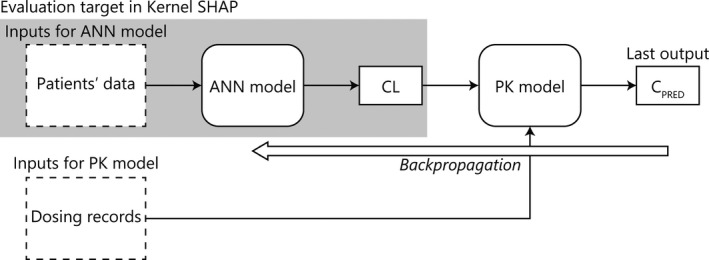
Basic structure of an artificial neural network pharmacokinetic model. SHAP, Shapley additive explanations; ANN, artificial neural network; CL, clearance; PK, pharmacokinetic; C_PRED, predicted values of cyclosporine concentration

Preprocessing of input data

Sex (SEX), age (AGE; year), body weight (WT; kg), alanine aminotransferase value (ALT; U/L), aspartate aminotransferase value (AST; U/L), and serum creatinine value (SCR; mg/dl) were used as the inputs for the ANN‐PK model. These inputs were standardized using the mean and SD of each input because the scale of each input value was different (Equation 2).

$$x_{\mathrm{std}}\left(i\right)=\frac{x\left(i\right)‐\overline{x}}{s_x}$$ (2)

$x_{\mathrm{std}}\left(i\right)$ and $x\left(i\right)$ represent the standardized or original values of i ^th data, respectively, and $\overline{x}$ and $s_x$ represent the mean and SD of feature x, respectively.

Cross validation and evaluation of model performance

The leave‐one‐out method was used as the cross validation for the ANN‐PK model (Figure S1). ²⁶ Of the 36 patients, 35 were assigned to the training data, and 1 patient was assigned to the test data. Training was performed 36 times to assign all 36 patients once to the test data. All parameters in the ANN were initialized before starting training, independent training was performed 36 times. The precision of model prediction was evaluated by the root mean squared error (RMSE; Equation 3) and goodness of fit (GOF) plots.

$$\mathrm{RMSE}=\sqrt{\frac{1}{n}\bullet \sum _{i=1}^n{\left(\widehat{y_i}‐y_i\right)}^2}$$ (3)

n represents the number of data items. $\widehat{y_i}$ and $y_i$ represent the predicted and observed drug concentrations of i ^th data, respectively.

Applying Kernel SHAP to explain the influence of patient data on CL

Kernel SHAP was applied to the trained model and SHAP values were calculated to evaluate the influence of each input on CL output by the ANN. ¹⁹ The Kernel SHAP was performed using KernelExplainer in the shap module (version 0.36.0).

RESULTS

Final ANN‐PK model

The final ANN model is shown in Figure 2. The ANN in the final model had 3 hidden layers, with the number of neurons being 30 units in the first layer and 60 units in the second and third layers. A parametric rectified linear unit was used as the activation function in the hidden layers. ²⁷ The GOF plots for the PopPK model and the final ANN‐PK model are compared in Figure 3. These plots represent observations versus predictions of drug concentrations, and plots were evenly distributed around y = x in each model. The RMSE for the PopPK model and the ANN‐PK model were 41.1 and 31.0 ng/ml, respectively. The coefficient of determination for these models was 0.932 for the PopPK model and 0.961 for the ANN‐PK model.

FIGURE 2.

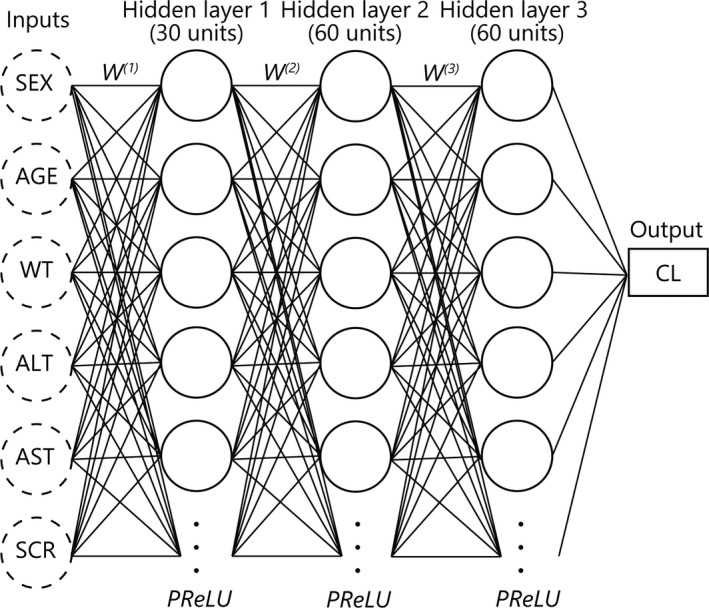
Structure of the final artificial neural network (ANN) model. The number of hidden layers in the final ANN model was three, and each layer consisted of 30, 60, and 60 units of neurons. The activation function in hidden layers was a parametric rectified linear unit (PReLU). SEX, sex; AGE, age (year); WT, body weight (kg); ALT, alanine aminotransferase (U/L); AST, aspartate transaminase (U/L); SCR, serum creatinine (mg/dl); W(n), nth weights in ANN model; PReLU, parametric rectified linear unit; CL, clearance

FIGURE 3.

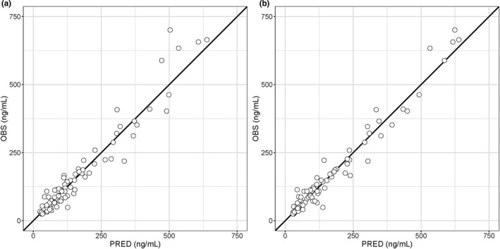
Goodness of fit plots for the population pharmacokinetic (PopPK) model and the artificial neural network pharmacokinetic (ANN‐PK) model. Open circles represent observations (OBS) versus predictions (PRED) by the PopPK model (a) and the ANN‐PK model (b), and solid lines represent y = x

Influence of patient data on CL

The results of evaluating the influence of inputs on output of CL using Kernel SHAP in 10 of 36 training sets are shown in Figures 4 and 5, and the results for all 36 training sets are shown in Figures S2 and S3. Bar‐plots in Figure 4 represent the mean of the absolute SHAP value (MEAN_[SHAP]) for each input. As the MEAN_[SHAP] for AGE was largest in 21 of 36 training sets, the influence of AGE on output of CL was the largest for 6 types of inputs. Moreover, AGE was the most influential input, followed by WT in 18 of the 36 training sets. Colored plots in Figure 5 represent SHAP values, and red and blue plots represent larger and smaller values, respectively. In the plots for AGE, red points were distributed in the range of negative SHAP values, indicating that the output CL values were smaller with higher AGE. On the other hand, for WT, red points were distributed in the range of the positive SHAP values, indicating that output CL values were larger for higher WT.

FIGURE 4.

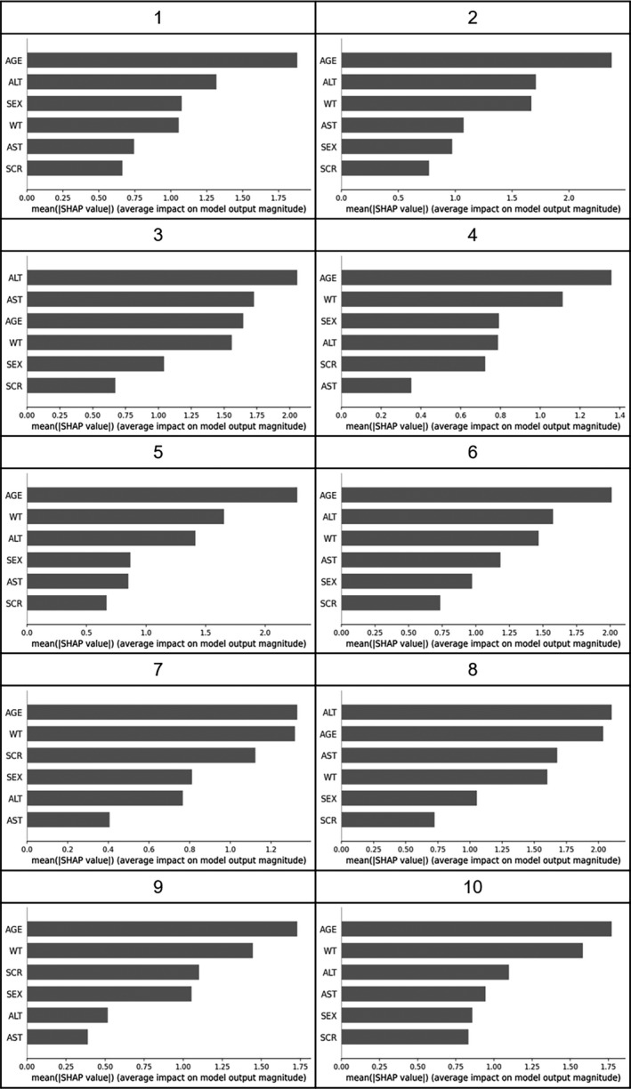
Summary bar‐plot of Kernel Shapley additive explanations (SHAP) in 10 of 36 training sets. Bar plot represents mean value of absolute SHAP values for each input in 10 of 36 training sets. ALT, alanine aminotransferase (U/L); AST, aspartate transaminase (U/L); AGE, age (year); WT, body weight (kg); SEX, sex (1 for male and 0 for female); SCR, serum creatinine (mg/dl)

FIGURE 5.

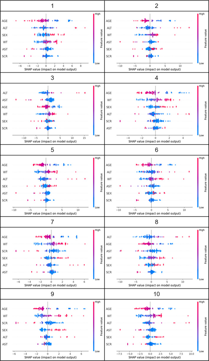
Summary plots of Kernel Shapley additive explanations (SHAP) in 10 of 36 training sets. The influence of each input on estimating clearance (CL) in 10 of 36 training sets is shown as colored plots. Red or blue plots represent higher or lower values of inputs, respectively. If the red plot is in the positive range of SHAP values, the higher CL value was the output with the higher input value. ALT, alanine aminotransferase (U/L); AST, aspartate transaminase (U/L); AGE, age (year); WT, body weight (kg); SEX, sex (1 for male, and 0 for female); SCR, serum creatinine (mg/dl)

DISCUSSION

In this study, the ANN‐PK model to predict time‐series cyclosporin A concentrations was constructed by using a simple ANN model in combination with a conventional compartment model. The application of Kernel SHAP to the constructed model allowed us to evaluate the influence of each input value on the output of the PK parameter.

Hold‐out methods or cross‐validation methods, such as the k‐fold and leave‐one‐out methods, are generally used for evaluating the performance of machine‐learning models. ²⁶ Using the leave‐one‐out method is recommended when the available data size is small; thus, the performance of the ANN‐PK model was evaluated using this cross‐validation method.

The RMSE for the PopPK model and the final ANN‐PK model were 41.1 and 31.0 ng/ml, respectively, and the prediction accuracy of drug concentrations increased by applying the ANN. The GOF plots for the ANN‐PK model represented more convergence to y = x compared with that for the PopPK model, with good model performance for the ANN‐PK model (Figure 3). For the PopPK model, the data for all 36 patients were used for the model building and the prediction accuracy was evaluated with the same data, whereas the data for 35 of the 36 patients were used for training of the ANN‐PK model. Therefore, the prediction accuracy of the ANN‐PK model was better despite the use of fewer patients for training. This indicates the usefulness of ANN for predicting drug concentrations.

When the PopPK model is built, the complexity of the model should be considered to prevent overfitting of the data used for parameter estimation. The presence of multiple units and hidden layers in the ANN models enable the feature learning of the input data by themselves. Thus, the advantage of using the ANN model was determined through its complexity. This implies that it is difficult to simply compare and evaluate the complexity of the PopPK and ANN models, because only the prediction performance was compared in this study. To confirm that overtraining did not occur in the ANN‐PK model, the leave‐one‐out method was performed and the loss function in the test data was monitored (Figure S4).

The most influential factors on CL output were AGE and WT from the evaluation using Kernel SHAP. These factors were incorporated into the PopPK model as the significant covariates of CL, so that the results from this study were consistent with those of the previous study. ²⁴ Figure 5 suggests that the output CL values decreased with increasing AGE and increased with increasing WT. It has been reported that the elimination of cyclosporine from blood is age‐dependent and the CL is large in younger patients. ²⁸ , ²⁹ It is also generally known that the basal metabolism increases in proportion to the 3/4 power of body weight. ³⁰ Therefore, the results of the Kernel SHAP evaluation were scientifically and biologically appropriate.

The interaction between PK parameters should be considered when predicting drug concentrations in the blood. In this study, the CL output from the ANN‐PK model was substituted for the compartment model, and the weights (parameters) in the ANN‐PK model were updated based on the predicted concentrations calculated from the compartment model. Therefore, the interaction between CL and volume of distribution (Vd) in the ANN‐PK model could be considered the same as that in the PopPK analysis when first‐order absorption rate constant (Ka) and Vd were fixed. It is also possible to have both CL and Vd simultaneously as outputs using the ANN model, in which case the interaction between CL and Vd is expected to be the same as when estimating both CL and Vd in the PopPK analysis. However, to evaluate the interaction numerically and visually in the ANN model, developing a novel evaluation method is necessary, as well as applying SHAP to visualize the influence of patient data on CL, which we will address in our future work.

Although the ANN model alone can predict drug blood concentrations, there are two advantages to using it in combination with the conventional compartment model. First, this prevents the model from becoming a complete black‐box model from input to output. In the present study, the influences of inputs were also evaluated using SHAP, but when the output from the ANN is drug concentrations, it is not possible to determine which phase of PKs (absorption, distribution, or elimination) is affected by the input. By using the output of the ANN as the PK parameters, it is possible to separately evaluate the influence of the inputs on each PK parameter. The second advantage was that we could handle the time‐series data. This was difficult to do with the ANN, and the sampling timing was fixed in the previous study which applied the ANN to predict drug concentrations. ⁹ It is possible to predict drug concentrations at any time, or in multiple dosing by using the compartment model to calculate the drug concentrations.

SHAP was used as the method to evaluate the influence of input on output by the ANN. SHAP has three desirable properties: (1) local accuracy, (2) missingness, and (3) consistency. ¹⁹ The trained model and the input were denoted by f(x) and x, respectively. The model used to explain the influence of each input and the simplified input denoted them as g(z) and z, respectively. When g(z) is expressed as the sum of the contributions of each input, “local accuracy” requires that f(x) matches g(z), that is, the sum of the contributions of each input matches f(x). “Missingness” is the property that the contribution of features not used to predict the model will be zero. “Consistency” requires that the importance of features in the two different models be consistent with the contribution of these features. In addition, SHAP does not need to incorporate a model explaining the contribution of the features at training, and it is possible to evaluate the influence of inputs after the training. ¹⁹ Thus, we can build a simple and highly expandable model for other drugs.

The limitation of this study was that the size of data was small. This is a common limitation for any drug because the size of data used for pharmacometrics is smaller than the training data used in other fields. There are two major issues in using small datasets for training machine learning models: (1) the model performance will be decreased compared to when training is performed with larger datasets; and (2) the risk of overtraining (overfitting) will increase. ³¹ , ³² , ³³ The first problem is common for PopPK modeling as well as neural network models, and both the ANN‐PK and PopPK models will show better model performance when larger datasets are available for model building. A previous study addressing a medical image identification problem showed that the accuracy of classification increased from 50% to over 95% when the number of training data was increased from 120 to 1200 images. ³² In this study, we performed a relative evaluation by comparing the performance between the ANN‐PK and PopPK models instead of performing an absolute evaluation. To prevent overtraining, the leave‐one‐out method was used for cross‐validation, and the losses in the test data were checked (Figure S4). Overtraining rarely occurred in this study, and this may have been due to the use of the compartment model, which inhibits learning that is largely out of line. Therefore, it may be effective to limit learning to avoid overlearning when applying artificial intelligence and machine learning to pharmacometrics. Another limitation was that our study was only performed in cyclosporin A. To ensure the usefulness of the method suggested in this study, further evaluation of other drugs and prediction of their pharmacodynamics, such as clinical efficacy and toxicity, is necessary.

The ANN‐PK model developed in this study could handle time‐series data and showed higher prediction accuracy than the conventional PopPK model used in predicting cyclosporin A concentrations. The scientific validity of the model was evaluated by applying SHAP to calculate the contribution of each input to the output of the PK parameter. Further study using other drugs and the prediction of pharmacodynamics are necessary to ensure the usefulness of the method developed in this study.

CONFLICTS OF INTEREST

The authors declared no competing interests for this work.

AUTHOR CONTRIBUTIONS

C.O., Y.T., and H.S. wrote the manuscript. C.O., Y.T., H.S., H.K., H.T., Y.M., and H.H. designed the research. C.O., Y.T., and H.S. performed the research. C.O., Y.T., and H.S., analyzed the data.

Supporting information

Fig S1

Fig S2

Fig S3

Fig S4

Table S1

REFERENCES

- 1. Hamet P, Tremblay J. Artificial intelligence in medicine. Metabolism. 2017;69S:S36‐S40. [DOI] [PubMed] [Google Scholar]
- 2. Harris M, Qi A, Jeagal L, et al. A systematic review of the diagnostic accuracy of artificial intelligence‐based computer programs to analyze chest x‐rays for pulmonary tuberculosis. PLoS One. 2019;14(9):e0221339. [DOI] [PMC free article] [PubMed] [Google Scholar]
- 3. Schneider G. Automating drug discovery. Nat Rev Drug Discov. 2017;17(2):97‐113. [DOI] [PubMed] [Google Scholar]
- 4. Yang X, Wang Y, Byrne R, Schneider G, Yang S. Concepts of artificial intelligence for computer‐assisted drug discovery. Chem Rev. 2019;119(18):10520‐10594. [DOI] [PubMed] [Google Scholar]
- 5. Wang N, Chen J, Xiao H, Wu L, Jiang H, Zhou Y. Application of artificial neural network model in diagnosis of Alzheimer's disease. BMC Neurol. 2019;19(1):154. [DOI] [PMC free article] [PubMed] [Google Scholar]
- 6. Yamashita F, Fujita A, Sasa Y, Higuchi Y, Tsuda M, Hashida M. An evolutionary search algorithm for covariate models in population pharmacokinetic analysis. J Pharm Sci. 2017;106(9):2407‐2411. [DOI] [PubMed] [Google Scholar]
- 7. Niel O, Bastard P. Artificial intelligence improves estimation of tacrolimus area under the concentration over time curve in renal transplant recipients. Transpl Int. 2018;31(8):940‐941. [DOI] [PubMed] [Google Scholar]
- 8. Thishya K, Vattam KK, Naushad SM, Raju SB, Kutala VK. Artificial neural network model for predicting the bioavailability of tacrolimus in patients with renal transplantation. PLoS One. 2018;13(4):e0191921. [DOI] [PMC free article] [PubMed] [Google Scholar]
- 9. Yamamura S, Kawada K, Takehira R, et al. Artificial neural network modeling to predict the plasma concentration of aminoglycosides in burn patients. Biomed Pharmacother. 2004;58(4):239‐244. [DOI] [PubMed] [Google Scholar]
- 10. Freitas AA, Limbu K, Ghafourian T. Predicting volume of distribution with decision tree‐based regression methods using predicted tissue:plasma partition coefficients. J Cheminform. 2015;7:1‐17. [DOI] [PMC free article] [PubMed] [Google Scholar]
- 11. LeCun Y, Bengio Y, Hinton G. Deep learning. Nature. 2015;521(7553):436‐444. [DOI] [PubMed] [Google Scholar]
- 12. Chen H, Engkvist O, Wang Y, Olivecrona M, Blaschke T. The rise of deep learning in drug discovery. Drug Discov Today. 2018;23(6):1241‐1250. [DOI] [PubMed] [Google Scholar]
- 13. Suzuki K. Overview of deep learning in medical imaging. Radiol Phys Technol. 2017;10(3):257‐273. [DOI] [PubMed] [Google Scholar]
- 14. Zihni E, Madai VI, Livne M, et al. Opening the black box of artificial intelligence for clinical decision support: a study predicting stroke outcome. PLoS One. 2020;15(4):e0231166. [DOI] [PMC free article] [PubMed] [Google Scholar]
- 15. Holzinger A, Langs G, Denk H, Zatloukal K, Muller H. Causability and explainability of artificial intelligence in medicine. Wiley Interdiscip Rev Data Min Knowl Discov. 2019;9(4):e1312. [DOI] [PMC free article] [PubMed] [Google Scholar]
- 16. Wang F, Kaushal R, Khullar D. Should health care demand interpretable artificial intelligence or accept "black box" medicine? Ann Intern Med. 2020;172(1):59‐60. [DOI] [PubMed] [Google Scholar]
- 17. Gregor K, Danihelka I, Graves A, Rezende DJ, Wierstra D. DRAW: a recurrent neural network for image generation. Proceedings of the 32nd International Conference on Machine Learning; Lille, France, 2015
- 18. Bach S, Binder A, Montavon G, Klauschen F, Muller KR, Samek W. On pixel‐wise explanations for non‐linear classifier decisions by layer‐wise relevance propagation. PLoS One. 2015;10(7):e0130140. [DOI] [PMC free article] [PubMed] [Google Scholar]
- 19. Lundberg SM, Lee S. A unified approach to interpreting model predictions. 31st Conference on Neural Information Processing Systems; Long Beach, CA, USA 2017.
- 20. Ribeiro MT, Singh S, Guestrin C. "Why Should I Trust You?". Proceedings of the 22nd ACM SIGKDD International Conference on Knowledge Discovery and Data Mining, 2016. pp. 1135–1144.
- 21. Bohanec M, Bratko I. Trading accuracy for simplicity in decision trees. Mach Learn. 1994;15:223‐250. [Google Scholar]
- 22. Chao LI, Wen‐hui Z, Ran LI, Jun‐yi W, Ji‐ming LIN. Research on star/galaxy classification based on stacking ensemble learning. Chin Astron Astrophy. 2020;44(3):345‐355. [Google Scholar]
- 23. Cao D‐S, Huang J‐H, Liang Y‐Z, Xu Q‐S, Zhang L‐X. Tree‐based ensemble methods and their applications in analytical chemistry. TrAC, Trends Anal Chem. 2012;40:158‐167. [Google Scholar]
- 24. Tsuji Y, Iwanaga N, Mizoguchi A, et al. Population pharmacokinetic approach to the use of low dose cyclosporine in patients with connective tissue diseases. Biol Pharm Bull. 2015;38(9):1265‐1271. [DOI] [PubMed] [Google Scholar]
- 25. Kingma DP, Ba JL. Adam: a method for stochastic optimization. The 3rd International Conference for Learning Representations; San Diego, CA, 2015.
- 26. Wong T‐T. Performance evaluation of classification algorithms by k‐fold and leave‐one‐out cross validation. Pattern Recogn. 2015;48(9):2839‐2846. [Google Scholar]
- 27. He K, Zhang X, Ren S, Sun J. Delving deep into rectifiers: surpassing human‐level performance on ImageNet classification. 2015 IEEE International Conference on Computer Vision (ICCV), 2015. pp. 1026–1034.
- 28. Yee G, McGuire T, Gmur D, Lennon T, Deeg H. Blood cyclosporine pharmacokinetics in patients undergoing marrow transplantation. Influence of age, obesity, and hematocrit. Transplantation. 1988;46(3):399‐402. [DOI] [PubMed] [Google Scholar]
- 29. Yee G, Lennon T, Gmur D, Kennedy M, Deeg H. Age‐dependent cyclosporine: pharmacokinetics in marrow transplant recipients. Clin Pharmacol Ther. 1986;40(4):438‐443. [DOI] [PubMed] [Google Scholar]
- 30. Holford NHG, Anderson BJ. Allometric size: the scientific theory and extension to normal fat mass. Eur J Pharm Sci. 2017;109S:S59‐S64. [DOI] [PubMed] [Google Scholar]
- 31. Ajiboye AR, Abdullah‐Arshah R, Qin H, Isah‐Kebbe H. Evaluating the effect of dataset size on predictive model using supervised learning technique. Int J Comp Syst Softw Eng. 2015;1(1):75‐84. [Google Scholar]
- 32. Cho J, Lee K, Shin E, Choy G, Do S. How Much Data is Needed to Train a Medical Image Deep Learning System to Achieve Necessary High Accuracy? ICLR 2016. San Juan, Puerto Rico: 2015. [Google Scholar]
- 33. Vabalas A, Gowen E, Poliakoff E, Casson AJ. Machine learning algorithm validation with a limited sample size. PLoS One. 2019;14(11):e0224365. [DOI] [PMC free article] [PubMed] [Google Scholar]
Associated Data
This section collects any data citations, data availability statements, or supplementary materials included in this article.
Supplementary Materials