Block-Based Statistics for Robust Non-parametric Morphometry

Abstract

Automated algorithms designed for comparison of medical images are generally dependent on a sufficiently large dataset and highly accurate registration as they implicitly assume that the comparison is being made across a set of images with locally matching structures. However, very often sample size is limited and registration methods are not perfect and may be prone to errors due to noise, artifacts, and complex variations of brain topology. In this paper, we propose a novel statistical group comparison algorithm, called block-based statistics (BBS), which reformulates the conventional comparison framework from a non-local means perspective in order to learn what the statistics would have been, given perfect correspondence. Through this formulation, BBS (1) explicitly considers image registration errors to reduce reliance on high-quality registrations, (2) increases the number of samples for statistical estimation by collapsing measurements from similar signal distributions, and (3) diminishes the need for large image sets. BBS is based on permutation test and hence no assumption, such as Gaussianity, is imposed on the distribution. Experimental results indicate that BBS yields markedly improved lesion detection accuracy especially with limited sample size, is more robust to sample imbalance, and converges faster to results expected for large sample size.

1. Introduction

Magnetic resonance imaging (MRI) is a powerful tool for in vivo detection of structural differences associated with diseases. A common approach taken by traditional voxel-based morphometry (VBM) [1] is to compare two sets of images, typically images from the patient population and the healthy population, voxel-by-voxel. Such comparison can either be done at a group level or at an individual level. The former aims at characterizing the overall cause of a disease whereas the latter focuses on detecting its early signs and, possibly, its future evolution.

To correct for structural variations between individuals, many MRI data comparison methods depend on large-scale, high-quality registrations. In fact, many methods inherently assume perfect alignment between images, which is seldom possible in real practice. Registration methods are not perfect and may be prone to errors due to noise, artifacts, and complex variations of brain topology. Registration error reduces the reliability of statistical comparison outcomes since detections and misdetections might be due to comparisons between mismatched structures. This stringent requirement on registration can be somehow relaxed by smoothing the images, e.g., by a Gaussian kernel, prior to comparison. This will however eliminate subtle details in the images and finer pathologies are hence elusive and might not be detected. Increasing sample size might help suppress random misalignment errors, but will at the same time reduce the possibility of detecting pathologies associated with systematically misaligned structures. The appropriate modeling of misalignment errors in statistical comparison methods is not only important for more accurate comparisons, but is also important to make full use of available samples and improve the statistical power in detecting fine-grained abnormalities associated with diseases.

Statistical comparison of MRI data usually relies on parametric or permutation statistical tests, which often require large databases to produce reliable outcomes. However, in medical imaging studies, a large sample size is often difficult to obtain due to low disease prevalence, recruitment difficulties, and data matching issues. To simplify the task of estimating the distribution of a static of interest, very often the distribution is assumed to be Gaussian and the task of distribution estimation is hence reduced to the estimation of model parameters. This Gaussianity assumption, however, often does not hold, especially for higher-order non-linear quantities whose distributions have unknown forms and are too complex to be modeled by simple Gaussians.

In this paper, we will introduce a robust technique, called block-based statistics (BBS), for group comparisons using small noisy databases. BBS unites the strengths of permutation test [2] and non-local estimation [3]. Permutation test makes little assumption about the distribution of a test statistic and allows a non-parametric determination of group differences. Non-local estimation uses a block matching mechanism to locate similar realizations of similar signal processes to significantly boost estimation efficacy. Through our evaluations using synthetic data and real data, we found that such combination allows accurate detection of group differences with a markedly smaller number of samples, allows greater robustness to sample imbalance, and improves speed of convergence to results expected for large sample size.

2. Approach

BBS entails a block matching component, which corrects for alignment errors, and a permutation testing component, where matching blocks are used for effective non-parametric statistical inference.

2.1. Block Matching

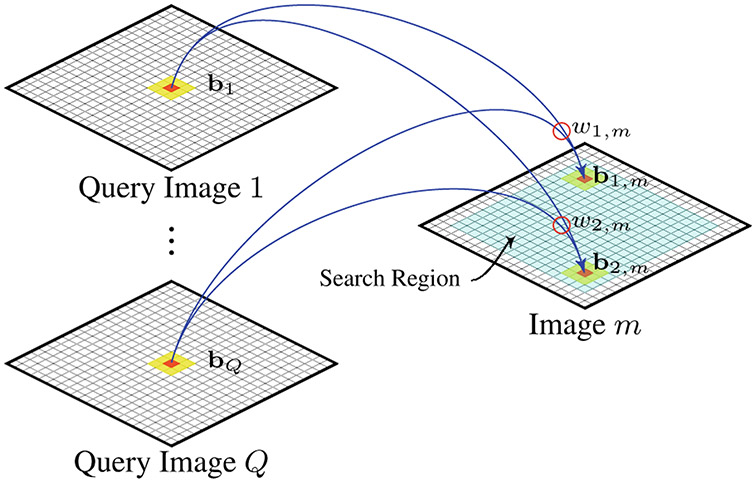
To deal with misalignment, block matching is used to determine similar structures for comparison purposes. Restricting statistical comparisons to only matched blocks will encourage comparison of similar and not mismatched information (e.g., due to structural misalignment). For group comparison, block matching is facilitated by a set of query images that are representative of each group. This is to avoid the bias involved in only using any single image from each group as the reference for block matching. When the group size is small, the query set consists of all images in each group. When the group size is large, a small number of query images representing different cluster centers can be selected with the help of a clustering algorithm. For any image in the group, blocking matching is performed with respect to the query images (see Fig. 1). That is, at each location in the common space of the query images, a set of blocks are concurrently compared with a block in the image.

Fig. 1. Block Matching.

Block matching is performed based on a set of query images. Each block b_{i, m} within the search region in an image m is compared with block set {b_q∣q = 1, 2, … , Q}. The weight w_i,m indicates the degree of similarity between b_i,m and {b_q}.

We assume that two groups of images (i.e., M₁ images $I_{m_1\in \{1,\dots ,M_1\}}^{[1]}$ in the first group and M₂ images $I_{m_2\in \{1,\dots ,M_2\}}^{[2]}$ in the second group), which can be vector-valued, have been registered to the common space. We are interested in comparing voxel-by-voxel images in the first group with the images in the second group. For each point $\mathbf{x}\in {\mathbb{R}}^3$ in the common space defined by the query images of the two groups, we define a common block neighborhood $\mathcal{N}(\mathbf{x})$ and arrange the elements (e.g., intensity values) of the voxels in this block neighborhood lexicographically as two sets of vectors $\{{\mathbf{b}}_{q_1}^{[1]}\in {\mathbb{R}}^d\mid q_1=1,2,\dots ,Q_1\}$ and $\{{\mathbf{b}}_{q_2}^{[2]}\in {\mathbb{R}}^d\mid q_2=1,2,\dots ,Q_2\}$, where Q_g is the number of query images in group g ∈ {1, 2}. Block matching is then performed as follows:

1. For each image $I_{m_1}^{[1]}$, search for blocks $\{{\mathbf{b}}_{i_1,m_1}^{[1]}\mid i_1=1,2,\dots \}$ that are similar to block set $\{{\mathbf{b}}_{q_1}^{[1]}\}$. Do the same for each $I_{m_2}^{[2]}$ using $\{{\mathbf{b}}_{q_2}^{[2]}\}$ as the reference to obtain blocks $\{{\mathbf{b}}_{i_2,m_2}^{[2]},\mid i_2=1,2,\dots \}$.

2. Assign a weight $w_{i_1,m_1}^{[1]}$ to the central voxel of each block ${\mathbf{p}}_{i_1,m_1}^{[1]}$ of each block ${\mathbf{b}}_{i_1,m_1}^{[1]}$, depending on the similarity between ${\mathbf{b}}_{i_1,m_1}^{[1]}$ and $\{{\mathbf{b}}_{q_1}^{[1]}\}$. Similarly, assign a weight $w_{i_2,m_2}^{[2]}$ to the central voxel ${\mathbf{p}}_{i_2,m_2}^{[2]}$ of each block ${\mathbf{b}}_{i_2,m_2}^{[2]}$.

3. Utilize the set of weighted samples $\{(w_{i_1,m_1}^{[1]},{\mathbf{p}}_{i_1,m_1}^{[1]})\mid i_1=1,2,\dots ;m_1=1,2,\dots ,M_1\}$ and $\{(w_{i_2,m_2}^{[2]},{\mathbf{p}}_{i_2,m_2}^{[2]})\mid i_2=1,2,\dots ;m_2=1,2,\dots M_2\}$ to infer the differences between $\{I_{m_1}^{[1]}\mid m_1=1,2,\dots ,M_1\}$ and $\{I_{m_2}^{[2]}\mid m_2=1,2,\dots ,M_2\}$.

The weight is defined as

$$w_{i_g,m_g}^{[g]}={\left[\prod _{q_g=1}^{Q_g}{K}_{\mathbf{H}}\left(\left[\begin{array}{c}\hfill {\mathbf{b}}_{i_g,m_g}^{[g]}\hfill \\ \hfill {\mathbf{x}}_i\hfill \end{array}\right]-\left[\begin{array}{c}\hfill {\mathbf{b}}_{q_g}^{[g]}\hfill \\ \hfill \mathbf{x}\hfill \end{array}\right]\right)\right]}^{\frac{1}{Q_g}},$$ (1)

where K_H = ∣H∣⁻¹K(H⁻¹•) is a multivariate kernel function with symmetric positive-definite bandwidth matrix H [4,5]. The weight indicates the similarity between a pair of blocks in a (d + 3)-dimensional space. This framework has several advantages: it can help correct for potential registration errors between images, and it can significantly increase the number of samples required for performing voxel-wise comparison. Statistical power can also be improved since the confounding variability due to misalignment can be reduced.

2.2. Permutation Test

We assume that the weighted samples ${\mathbf{Z}}^{[1]}=\{(w_{i_1,m_1}^{[1]},{\mathbf{p}}_{i_1,m_1}^{[1]})\}$ and ${\mathbf{Z}}^{[2]}=\{(w_{i_2,m_2}^{[2]},{\mathbf{p}}_{i_2,m_2}^{[2]})\}$ determined previously are independent random samples drawn from two possibly different probability distributions F^[1] and F^[2]. Our goal is to test the null hypothesis H₀ of no difference between F^[1] and F^[2], i.e., H₀ : F^[1] = F^[2]. A hypothesis test is carried out to decide whether or not the data decisively reject H₀. This requires a test statistic $\widehat{\theta }=s({\mathbf{Z}}^{[1]},{\mathbf{Z}}^{[2]})$, such as the difference of means. In this case, the larger value of the statistic, the stronger is the evidence against H₀. If the null hypothesis H₀ is not true, we expect to observe larger values of $\widehat{\theta }$ than if H₀ is true. The hypothesis test of H₀ consists of computing the achieved significance level (ASL) of the test, and seeing if it is too small according to certain conventional thresholds. Having observed $\widehat{\theta }$, the ASL is defined to be the probability of observing at least that large a value when the null hypothesis is true: $\text{ASL}={\text{Prob}}_{H_0}\{{\widehat{\theta }}^{\ast }\ge \widehat{\theta }\}$. The smaller the value of ASL, the stronger the evidence against H₀.

The permutation test assumes that under null hypothesis F^[1] = F^[2], the samples in both groups could have come equally well from either of the distributions. In other words, the labels of the samples are exchangeable. Therefore the null hypothesis distribution can be estimated by combining all the N₁ + N₂ samples from both groups into a pool and then repeating the following process for a large number of times B:

1. Take N₁ samples without replacement to form the first group, i.e., Z*^[1], and leave the remaining N₂ samples to form the second group, i.e., Z*^[2].

2. Compute a permutation replication of $\widehat{\theta }$, i.e., ${\widehat{\theta }}^{\ast }=s({\mathbf{Z}}^{\ast [1]},{\mathbf{Z}}^{\ast [2]})$.

The null hypothesis distribution is approximated by assigning equal probability on each permutation replication. The ASL is then computed as the fraction of the number of ${\widehat{\theta }}^{\ast }$ that exceeds θ: $\text{ASL}=\#\{{\widehat{\theta }}^{\ast }\ge \widehat{\theta }\}∕B$.

2.3. Choice of Kernel

A variety of kernel functions are possible in general [6]. Consistent with non-local means [3], we use a Gaussian kernel, i.e., $K(\mathbf{u})=\alpha \text{exp}\left(-\frac{1}{2}{\mathbf{u}}^{\mathrm{T}}\mathbf{u}\right)$, and hence $K_{\mathbf{H}}(\mathbf{u})=\mid \mathbf{H}{\mid }^{-1}K({\mathbf{H}}^{-1}\mathbf{u})=\frac{\alpha }{\mid \mathbf{H}\mid }\text{exp}\left(-\frac{1}{2}{\mathbf{u}}^{\mathrm{T}}{\mathbf{H}}^{-2}\mathbf{u}\right)$, where α is a constant to ensure unit integral. The choice of H is dependent on the application. For simplicity, we set $\mathbf{H}=\text{diag}(h_1^{[\mathbf{b}]},\dots ,h_d^{[\mathbf{b}]},h_1^{[\mathbf{x}]},\dots ,h_3^{[\mathbf{x}]})$ with $h_k^{[\mathbf{b}]}=\sigma \sqrt{d}$. The noise level σ can be estimated by the method outlined in [7]. We set $h_k^{[\mathbf{x}]}$ to be half the value of the search radius.

3. Experiments

We evaluated the effectiveness of BBS in detecting group differences using synthetic and real in vivo diffusion MRI data. The standard permutation test [2] was used as the comparison baseline. Group comparison was performed voxel-wise by the sum of squared differences (SSD) of the means, i.e., $\widehat{\theta }(\mathbf{x})=\Vert {\overline{I}}^{[1]}(\mathbf{x})-{\overline{I}}^{[2]}(\mathbf{x}){\Vert }^2$. Note that more sophisticated statistics (e.g. Hotelling’s T²-statistic) can be applied here to improve performance. For the standard permutation test, the mean is computed simply by averaging across images in the same group. For BBS, the mean is computed instead using weighted averaging using the weighted samples, i.e.,

$${\overline{I}}^{[g]}(\mathbf{x})\equiv \frac{{\sum }_{(w_{i,m},{\mathbf{p}}_{i,m})\in {\mathbf{Z}}^{[g]}(\mathbf{x})}[w_{i,m}{]}^{M_g^{\gamma }}{\mathbf{p}}_{i,m}}{{\sum }_{(w_{i,m},{\mathbf{p}}_{i,m})\in {\mathbf{Z}}^{[g]}(\mathbf{x})}[w_{i,m}{]}^{M_g^{\gamma }}}.$$ (2)

The exponent $M_g^{\gamma }$, γ > 0, is for adjusting the weights according to the number of images. This is to reduce estimation bias when a greater number of images are available. According to [8], we set γ = 2/5. Note that if we restrict the search range to 1 × 1 × 1 and override the weights with 1, BBS is equivalent to the standard permutation test. For all experiments, we set the search range to 5 × 5 × 5 and the block size to 3 × 3 × 3. A search diameter of 5 is sufficient for correcting the registration errors because the images have already been nonlinearly aligned.

3.1. Synthetic Data

BBS was first evaluated using synthetic data. Based on a reference vector-valued diffusion-weighted image (each element corresponding to a diffusion gradient direction, see Fig. 2(a)), 10 replicates were generated by varying the locations, sizes, and principal diffusion directions of the ‘normal’ structures (squares) to form the ‘normal control’ dataset. Based on a ‘pathological’ reference image (see Fig. 2(b)), created by introducing lesions (‘circles’) to the reference image, a corresponding ‘patient’ dataset was generated by varying the locations, sizes, and severity of lesions, in addition to perturbing the normal structures as before. Lesions were simulated by swelling tensors in the non-principal directions. Group comparison was repeated using 10 Rician noise realizations of the datasets.

Fig. 2. Synthetic Data.

Noisy reference images with (A) normal structures (squares) and (B) lesions (circles). (C) Average image of 10 perturbed versions of (B). (D) Average image after block-matching correction.

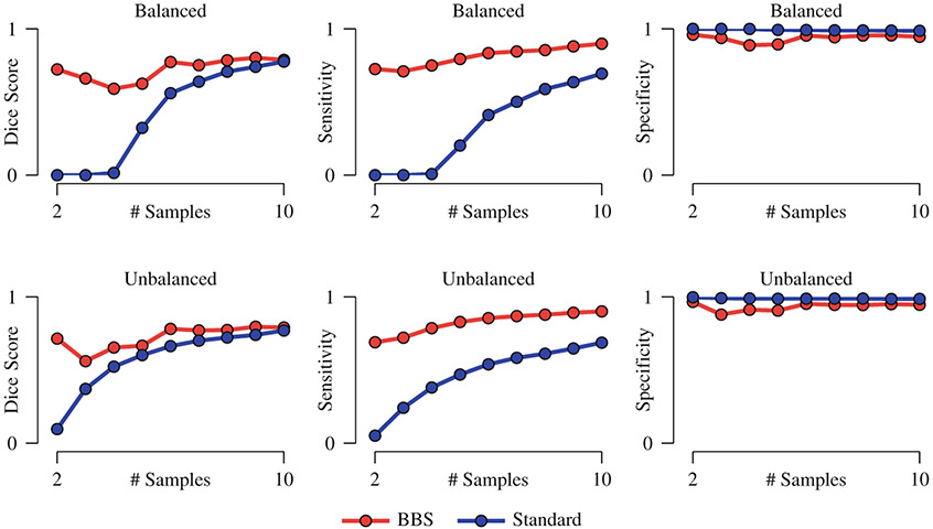
To demonstrate the power of BBS, we performed group comparison by progressively increasing the number of samples. Voxels with ASL < 0.01 were considered to be significantly different between the two groups. Detection accuracy was evaluated using Dice score with the lesions defined on the reference image as the baseline. Both cases of balanced and unbalanced sample sizes were considered. For the latter, only the size of the patient dataset was varied; the size of the normal control dataset was fixed at 10. The results, shown in Fig. 3, indicates that BBS yields markedly improved accuracy even when the sample size is small. Detection sensitivity is greatly increased by BBS. The specificity of both methods is comparable. The improvements given by BBS can be partly attributed to the fact that BBS explicitly corrects for alignment errors and yields sharper mean images than simple averaging, as can be observed from Fig. 2(c) and (d).

Fig. 3. Performance Statistics.

Detection accuracy, sensitivity, and specificity of BBS compared with the standard permutation test. The mean values of 10 repetitions are shown. The standard deviations are negligible and are not displayed. For the case of balanced sample size, both groups have the same number of samples. For the case of unbalanced sample size, only the size of the patient dataset was varied; the size of the normal control dataset was fixed at 10.

3.2. Real Data

Diffusion MR imaging was performed on a clinical routine whole body Siemens 3T Tim Trio MR scanner. We used a standard sequence: 30 diffusion directions isotropically distributed on a sphere at b = 1,000 s/mm², one image with no diffusion weighting, 128 × 128 matrix, 2 × 2 × 2 mm³ voxel size, TE = 81ms, TR = 7,618 ms, 1 average. Scans for 10 healthy subjects and 10 mild cognitive impairment (MCI) subjects were used for comparison. Before group comparison was performed, the scans were all non-linearly registered to a common space using a large deformation diffeomorphic registration algorithm [9,10].

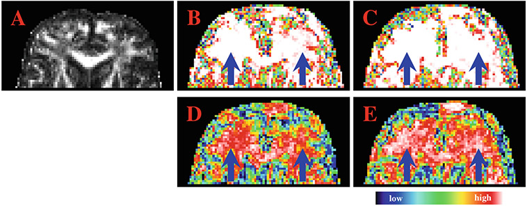
Representative qualitative comparison results are shown in Fig. 4. The color maps present the inverted ASL values, i.e., 1 – ASL, obtained by the two methods using 5 and 10 images in each group. Warmer and brighter colors indicate differences with greater significance. When a limited number of samples are available, BBS gives results that are more consistent with results obtained with a larger sample size. In the figure, the arrows mark the regions where the standard permutation test gives inconsistent results when different sample sizes are used.

Fig. 4. Achieved Significance Level.

Inverted ASL, i.e., 1 – ASL, obtained by BBS (B & C) and the standard permutation test (D & E) using 5 (B & D) and 10 (C & E) samples. The fractional anisotropy image (A) is shown for reference.

For quantitative evaluation, we used the detection results obtained using the full 10 samples as the reference and evaluated whether hypothesis testing using a smaller number of samples gives consistent results. The evaluation results shown in Fig. 5 indicate that BBS yields results that converge faster to the results given by a larger sample size. An implication of this observation is that BBS improves group comparison accuracy in small datasets.

Fig. 5. Performance Statistics for Real Data.

Detection accuracy, sensitivity, and specificity of BBS compared with the standard permutation test. The mean values of 10 repetitions are shown. The standard deviations are negligible and are not displayed.

4. Conclusion

We have presented a new method for detecting group differences with greater robustness. The method, called block-based statistics (BBS), explicitly corrects for alignment errors and shows greater detection accuracy and sensitivity compared with the standard permutation test, even when the number of samples is very low. The key benefits of BBS have been validated by the experimental results. In the future, we will improve the algorithm by using more sophisticated statistics and by incorporating resampling-based correction for multiple testing. BBS will also be applied to detect differences in quantities will greater complexity, such as orientation distribution functions and tractography streamlines.

References

- 1.Ashburner J, Friston KJ: Voxel-based morphometry - the methods. NeuroImage 11(6), 805–821 (2000) [DOI] [PubMed] [Google Scholar]
- 2.Efron B, Tibshirani RJ: An Introduction to the Bootstrap. Monographs on Statistics and Applied Probablilty. Chapman and Hall, Boca Raton: (1994) [Google Scholar]
- 3.Buades A, Coll B, Morel JM: A review of image denoising algorithms, with a new one. Multiscale Model. Simul. 4(2), 490–530 (2005) [Google Scholar]
- 4.Härdle W, Müller M: Multivariate and semiparametric kernel regression. In: Schimek MG (ed.) Smoothing and Regression: Approaches, Computation, and Application. Wiley, Hoboken: (2000) [Google Scholar]
- 5.Yap PT, An H, Chen Y, Shen D: Uncertainty estimation in diffusion MRI using the non-local bootstrap. IEEE Trans. Med. Imaging 33(8), 1627–1640 (2014) [DOI] [PMC free article] [PubMed] [Google Scholar]
- 6.Härdle W: Applied Nonparametric Regression. Cambridge University Press, Cambridge: (1992) [Google Scholar]
- 7.Manjón J, Carbonell-Caballero J, Lull J, García-Martí G, Martí-Bonmatí L, Robles M: MRI denoising using non-local means. Med. Image Anal 12(4), 514–523 (2008) [DOI] [PubMed] [Google Scholar]
- 8.Silverman B: Density Estimation for Statistics and Data Analysis. Monographs on Statistics and Applied Probablilty. Chapman and Hall, London: (1998) [Google Scholar]
- 9.Zhang P, Niethammer M, Shen D, Yap PT: Large deformation diffeomorphic registration of diffusion-weighted imaging data. Med. Image Anal. 18(8), 1290–1298 (2014) [DOI] [PMC free article] [PubMed] [Google Scholar]
- 10.Yap PT, Shen D: Spatial transformation of DWI data using non-negative sparse representation. IEEE Trans. Med. Imaging 31(11), 2035–2049 (2012) [DOI] [PMC free article] [PubMed] [Google Scholar]