Estimating Reference Bony Shape Models for Orthognathic Surgical Planning Using 3D Point-Cloud Deep Learning

Abstract

Orthognathic surgical outcomes rely heavily on the quality of surgical planning. Automatic estimation of a reference facial bone shape significantly reduces experience-dependent variability and improves planning accuracy and efficiency. We propose an end-to-end deep learning framework to estimate patient-specific reference bony shape models for patients with orthognathic deformities. Specifically, we apply a point-cloud network to learn a vertex-wise deformation field from a patient’s deformed bony shape, represented as a point cloud. The estimated deformation field is then used to correct the deformed bony shape to output a patient-specific reference bony surface model. To train our network effectively, we introduce a simulation strategy to synthesize deformed bones from any given normal bone, producing a relatively large and diverse dataset of shapes for training. Our method was evaluated using both synthetic and real patient data. Experimental results show that our framework estimates realistic reference bony shape models for patients with varying deformities. The performance of our method is consistently better than an existing method and several deep point-cloud networks. Our end-to-end estimation framework based on geometric deep learning shows great potential for improving clinical workflows.

I. Introduction

THE goal of orthognathic surgery is to correct deformed jaws and restore normal-looking facial appearances for patients with dentofacial deformities. The success of orthognathic surgery highly depends on a carefully designed surgical plan [1], [2]. In the planning process, a patient’s head computed tomography (CT) or cone-beam computed tomography (CBCT) scan is used to reconstruct a 3-dimensional (3D) shape model of the craniomaxillofacial (CMF) bony structure (Fig. 1(a)). The deformed jaw (Fig. 1(b)) of the CMF bone are then cut into multiple pieces (Fig. 1(c)) and each piece is translated and rotated to form a “new and normal” CMF bone. Currently, the outcome of this planning procedure largely relies on a surgeon’s subjective experience and 3D cephalometric analysis [3]. There is an urgent clinical need to develop an objective and automatic means of estimating a normal reference CMF bony shape model for efficient surgical planning.

Fig. 1.

(a) A 3D CMF bone model of a patient with dentofacial deformity. (b) The patient’s bones can be divided into a normal region marked as “midface” and a deformed region marked as “jaw”. (c) The deformed jaw is cut into five pieces, i.e., the Le Fort segment, right proximal segment, left proximal segment, distal segment, and chin segment.

Wang et al. [4] introduced a sparse representation method to estimate a patient-specific reference shape model. By representing the bony shape with a set of CMF landmarks, they construct midface and jaw landmark dictionaries based on a set of normal bones. By representing a patient’s midface landmarks using the normal midface dictionary, a set of sparse coefficients are calculated and then applied to the normal jaw dictionary to estimate the landmarks of the patient’s normal jaw. Using the original midface landmarks and estimated jaw landmarks, a deformation field is computed to warp the patient’s deformed bone and generate its normal shape model. This sparse representation method yields impressive performance when applied to synthetic datasets. However, its practical effectiveness is unclear due to the lack of rigorous evaluation on real clinical datasets. Moreover, its performance is determined by the quality of landmark digitization, which is a labor-intensive, error-prone, experience-dependent process.

Geometric deep learning [5] can be potentially utilized for reference bony shape estimation. The majority of geometric deep networks are developed for graph-structured data, with the most representative method being the Graph Convolution Network (GCN) designed for the spectral or spatial domain [6]. Spectral GCNs [7], [8] perform convolutions on graph data in the spectral domain with the help of an adjacency matrix. Spatial GCNs, e.g., MoNet [9], implement spatial convolutions in a local region for each node of the graph. Unlike GCNs, Qi et al. [10] proposed PointNet to work on point clouds with Multi-Layer Perceptrons (MLPs) shared across points. PointNet is a general framework for 3D data processing as a point cloud is more general than a graph. Qi et al. [11] further introduced PointNet++ by considering local point feature learning. This method leverages a hierarchical architecture to learn and integrate local point features and global shape information, achieving higher learning accuracy than PointNet without regional dependency modeling. PointNet++ has become a standard network for various point-cloud related tasks. A review of a series of more advanced point-cloud networks based on PointNet++ is provided in [12]. However, these methods are designed specifically for 3D classification and segmentation tasks. The feasibility of utilizing such techniques in automatic estimation of 3D shape models has not yet been investigated.

In this paper, for the first time, we apply geometric deep learning for reference bony shape estimation in orthognathic surgical planning. We propose an end-to-end deep learning framework based on a point-cloud network to estimate normal-looking 3D bony shape models for the patients with jaw deformities, without the need to predefine any CMF landmarks. Specifically, our network estimates a displacement field for correcting positions of vertices in a deformed shape model to generate a patient-specific reference shape model. Since paired deformed-normal CMF models are scarce, we design a strategy to simulate diverse jaw deformities from normal bones to train the network. The proposed method was comprehensively evaluated by using both synthetic and real patient data. We compared the proposed framework with the existing sparse representation method [4] and a number of point-cloud networks [11], [13]-[15]. Both qualitative and quantitative experimental results show that our approach achieves estimation performance superior over related methods.

The rest of the paper is organized as follows. We flesh out the details of our method in Section II, present experimental results in Section III, provide further discussion in Section IV, and conclude in Section V.

II. Methods

An overview of our method is provided in Fig. 2. Given a deformed bony surface, consisting of N vertices, i.e., V = {v₁, v₂, v₃,…, v_N}, we construct the point features f_i for each vertex v_i by stacking its coordinates $c_i=(c_x^i,c_y^i,c_z^i)$ and point normal $n_i=(n_x^i,n_y^i,n_z^i)$, i.e., $f_i=(c_x^i,c_y^i,c_z^i,n_x^i,n_y^i,n_z^i)$. Then, all point features F = {f₁, f₂, f₃,…, f_N} are fed into our Deformation Network (DefNet) to generate point-wise displacement vectors that are added to the coordinates of corresponding vertices of the original deformed bony surface to generate a corrected bony surface.

Fig. 2.

Schematic diagram of our method for reference bony shape estimation from a patient’s deformed bony shape. The deformed jaw for correction is labeled in red.

A. Network Architecture of DefNet

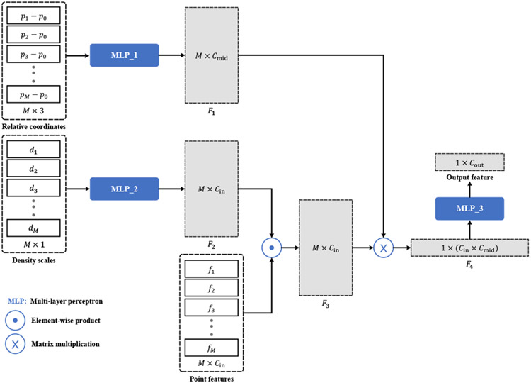
The encoder-decoder architecture of DefNet (Fig. 3) is derived from PointNet++ [11]. The encoder consists of a hierarchy of convolutional layers, each performing sampling, grouping, and convolution. The sampling operation selects a subset of N_sub points from the input points according to furthest point sampling [11]. After sampling, a local coordinate system is formed in the vicinity of each sampled point p₀, with the relative coordinates of each point p_i within a ball of radius r from p₀ calculated as p_i − p₀. In addition, to take into account the density of points surrounding p_i, a scale d_i is calculated using the method reported in [16]. Based on the relative coordinates and density scales, we perform convolution (Fig. 4) via the PointConv operator [17] to learn from the point features (i.e., f_i) a higher-level representation of the local shape.

Fig. 3.

The architecture of the deformation network (DefNet).

Fig. 4.

Convolution based on M neighboring points. The input consists of the relative coordinates {(p₁ − p₀), (p₂ − p₀), …, (p_M − p₀)}, the density scales {d₁, d₂, …, d_M}, and point features {f₁, f₂, …, f_M}. First, two multi-layer perceptrons (MLPs) are applied to the relative coordinates and density scales to learn the M × C_mid (C_mid = 32) distance weight matrix F₁ and the M × C_in (C_in = 6) density weight matrix F₂. Then, F₂ is multiplied element-wise with the point feature matrix to obtain the feature matrix F₃, which is further multiplied with F₁ and vectorized to produce a feature vector F₄ of length C_in × C_mid. The output feature vector of length C_out is obtained by applying a MLP to F₄.

Along the forward path of the encoder part, larger-scale features are progressively extracted and aggregated to capture global contextual information of the input point cloud. Mostly symmetric with respect to the encoder, the decoder consists of a group of deconvolutional layers. Each layer first performs upsampling to generate a denser point set via interpolation [11]. The learned features for the upsampled point set are concatenated with those from the corresponding encoder layer with skip connections. Grouping and convolution operations are then applied to the features of the upsampled point set, producing higher-level representations that integrate local and global information. Finally, the point-wise output of the decoder is processed by a set of MLPs shared across all points to produce a set of displacement vectors that are applied to the input points for deformity correction.

B. Loss Function

The loss function used to train our network is

$$L=L_{\text{vertex}}+L_{\text{face}}+\alpha L_{\text{reg}},$$ (1)

where L_vertex is the term quantifying the vertex-wise distance between the estimated and ground truth surfaces, i.e.,

$$L_{\text{vertex}}=\frac{1}{N_{\text{vertex}}}\sum _{i=1}^{N_{\text{vertex}}}{w}_i^{\text{vertex}}\Vert v_i^{\text{Est}}-v_i^{\text{GT}}{\Vert }_2,$$ (2)

in which N_vertex is the number of vertices on the surface, $v_i^{\text{Est}}$ is the i-th vertex on the estimated surface, $v_i^{\text{GT}}$ is the corresponding vertex from the ground truth surface, ${\Vert v_i^{\text{Est}}-v_i^{\text{GT}}\Vert }_2$ denotes the Euclidean distance between $v_i^{\text{Est}}$ and $v_i^{\text{GT}}$. The weight $w_i^{\text{vertex}}$ is calculated as

$$w_i^{\text{vertex}}=\text{exp}(\Vert v_i^{\text{Def}}-v_i^{\text{GT}}{\Vert }_2),$$ (3)

where $v_i^{\text{Def}}$ is the i-th vertex on the deformed bony surface. Since $w_i^{\text{vertex}}$ increases with the deformation magnitude, bony parts with larger deformities contribute more in (2). Complementary to L_vertex in measuring the surface distance in terms of vertices, we compute the distance between the corresponding faces on the estimated and ground truth surfaces:

$$L_{\text{face}}=\frac{1}{N_{\text{face}}}\sum _{j=1}^{N_{\text{face}}}{w}_j^{\text{face}}\Vert l_j^{\text{Est}}-l_j^{\text{GT}}{\Vert }_1,$$ (4)

where N_face is the number of faces, ∥·∥₁ denotes the ℓ₁-norm, and $l_j^{\text{Est}}$ and $l_j^{\text{GT}}$ are the perimeters of the j-th faces on the estimated and ground truth surfaces, respectively. Denoting using $v_{\text{face},j}^{\text{Def}}$ the center position of the j-th face on the deformed bony surface, and $v_{\text{face},j}^{\text{GT}}$ the center position of the corresponding face on the ground truth surface, the coefficient $w_j^{\text{face}}$ in (4) is calculated by

$$w_j^{\text{face}}=\text{exp}\left(\Vert v_{\text{face},j}^{\text{Def}}-v_{\text{face},j}^{\text{GT}}{\Vert }_2\right).$$ (5)

By minimizing (1), we encourage the network to learn a deformation held that only corrects the deformed portion (i.e., the jaw), but fixes the normal portion (i.e., the midface). To avoid overfitting, ℓ₂-norm regularization of the network parameters, denoted as L_reg, is included in the loss function, weighted by α = 0.5.

C. Generation of Training Data

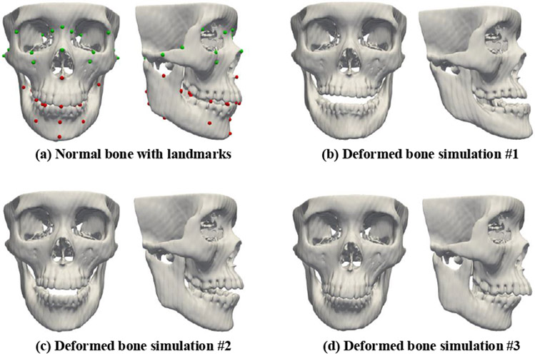
DefNet should ideally be trained using paired deformed and normal bony surfaces, which however can be difficult to acquire in practice. To generate paired training data, we simulate various deformed bones from normal bones using the sparse representation method similar to [4]. We represent a bony shape with midface and jaw landmarks (Fig. 5(a)) and then construct two landmark dictionaries (i.e., $D_{\text{mid}}^{\text{Pat}}$ and $D_{\text{jaw}}^{\text{Pat}}$) using the bony landmarks extracted from a set of real patients. For each normal bone, we represent its midface landmarks $L_{\text{mid}}^{\text{Norm}}$ with $D_{\text{mid}}^{\text{Pat}}$ in terms of a sparse coefficients vector C_min determined by

$$C_{\text{min}}=\underset{C}{\text{arg min}}\Vert D_{\text{mid}}^{\text{Pat}}C-L_{\text{mid}}^{\text{Norm}}{\Vert }_2^2+{\lambda }_1\Vert C{\Vert }_1+{\lambda }_2\Vert C{\Vert }_2,$$ (6)

where the parameters λ₁ and λ₂ control the sparsity, and ∥·∥₁ and ∥·∥₂ denote the ℓ₁-norm and ℓ₂-norm, respectively. Based on the calculated sparse coefficients C_min, the jaw landmarks $L_{\text{jaw}}^{\text{Est}}$ of the deformed bone simulated from the normal subject are determined by

$$L_{\text{jaw}}^{\text{Est}}=D_{\text{jaw}}^{\text{Pat}}{C}_{\text{min}}.$$ (7)

Fig. 5.

A normal facial bone and its three corresponding deformed bones simulated with the sparse representation method. Landmarks in the normal midface region and the deformed jaw region are marked respectively in green and red.

Next, $L_{\text{mid}}^{\text{Norm}}$ and $L_{\text{jaw}}^{\text{Est}}$ are combined to obtain the complete set of landmarks for the simulated deformed bone. Using the estimated and original bony landmarks, we calculate a dense deformation field using thin plate spline (TPS) interpolation [18]. The calculated deformation field is then applied to the original normal bony surface to generate the surface of the simulated deformed bone. We adjust the parameters λ₁ and λ₂ to simulate a set of different deformed bones for each normal subject (Fig. 5(b)-(d)). In this way, we produce a relatively large and diverse dataset of paired deformed-normal surfaces.

D. Network Training and Inference

In the training phase, we simplify each surface mesh [19] by reducing its number of vertices to improve computation efficiency. Coordinate values of surface vertices are min-max normalization before they are fed to the network. The network parameters are optimized by minimizing (1) with the Adam optimizer [20]. During the inference phase, we apply the trained network on a deformed bony shape without mesh simplification. Our network is not affected by the actual number of vertices on a testing surface.

III. Experimental Results

A. Experimental Data

To train the proposed network, we leveraged the head CT scans of 47 normal subjects, which were collected in a previous study [21], and the head CT scans from 61 patients with jaw deformities (collected under Institutional Review Board approval #Pro00009723). These scans were automatically segmented using the method described in [22] to extract bony masks. The bony surfaces were then generated from the mask images using the marching cubes algorithm [23]. A set of 51 anatomical cephalometric landmarks (Fig. 5(a)) routinely used in clinical practices were manually digitized by an experienced surgeon. These landmarks were used only for deformed bone simulation and quantitative performance evaluation. We adopted the method described in Section II-C to simulate 34 jaw deformities for each normal subject by leveraging the 61 patient bones as the dictionary. The deformities include, but are not limited to, maxillary and mandibular hypoplasia/hyperplasia, maxillary vertical excess, unilateral condylar hyperplasia, and anterior open bite. The simulated deformities were examined independently by two experienced oral surgeons.

B. Experimental Settings

For each training bony surface, the total number of vertices was reduced to N = 4,700 after surface mesh simplification (see Section II-D). The number of vertices on the testing bony surface varies from case to case, but N > 100,000. We employed 8 layers for DefNet with $N_{\text{sub}}=\{\frac{N}{4},\frac{N}{16},\frac{N}{64},\frac{N}{128},\frac{N}{64},\frac{N}{16},\frac{N}{4},N\}$ and r = {0.1, 0.2, 0.4, 0.8, 0.8, 0.4, 0.2, 0.1}. The dimension numbers of output point feature vectors in the 8 layers were set to C = {64, 128, 256, 512, 512, 256, 128, 128}.

C. Evaluation Metrics

We utilized four metrics for method evaluation, including vertex distance (VD), edge-length distance (ED), surface coverage (SC), and landmark distance (LD). VD is the average distance between corresponding vertices on the estimated and ground truth surfaces:

$$\text{VD}=\frac{1}{N_v}\sum _{i=1}^{N_v}\Vert v_i^{\text{Est}}-v_i^{\text{GT}}{\Vert }_2,$$ (8)

where N_v is the number of vertices on the estimated surface, $v_i^{\text{Est}}$ is the coordinates of the i-th vertex, and $v_i^{\text{GT}}$ is the coordinates of the corresponding i-th vertex on the ground truth surface. ED assesses how well mesh topology is preserved on the estimated bony surface:

$$\text{ED}=\frac{1}{N_e}\sum _{i=1}^{N_e}\Vert e_i^{\text{Est}}-e_i^{\text{GT}}{\Vert }_1,$$ (9)

where N_e is the number of edges on the estimated surface, and $e_i^{\text{Est}}$ and $e_i^{\text{GT}}$ are the lengths of the i-th corresponding edges on the estimated and ground truth surfaces, respectively. SC is defined as the ratio

$$\text{SC}=\frac{N_v^{\text{Closest}}}{N_v},$$ (10)

where $N_v^{\text{Closest}}$ is the number of vertices on the ground truth bony surface that are closest to the vertices on the estimated surface. N_v is the number of vertices on the ground truth surface. Larger SC indicates greater overlap between the estimated and ground truth surfaces. LD computes the distance of a set of landmark surface vertices:

$$\text{LD}=\frac{1}{N_l}\sum _{i=1}^{N_l}\Vert l_i^{\text{Est}}-l_i^{\text{GT}}{\Vert }_2,$$ (11)

where N_l = 51 is the number of the landmarks, and $l_i^{\text{Est}}$ and $l_i^{\text{GT}}$ denote the coordinates of the i-th corresponding landmarks on the estimated and ground truth surfaces, respectively.

D. Evaluation on Synthetic Data

Nine-fold cross-validation was conducted with the synthetic data to assess the performance of our method. That is, 1,598 paired deformed-normal bones generated from the 47 normal subjects were divided into 9 groups with approximately 170 pairs in each group. Eight groups were used for network training and one for testing. The synthetic samples from a normal subject appear either in the training set or the testing set, but not both. The performance was evaluated by directly comparing the estimated bony surface with the corresponding normal bony surface as ground truth. We compared DefNet with the sparse representation (SR) method [4].

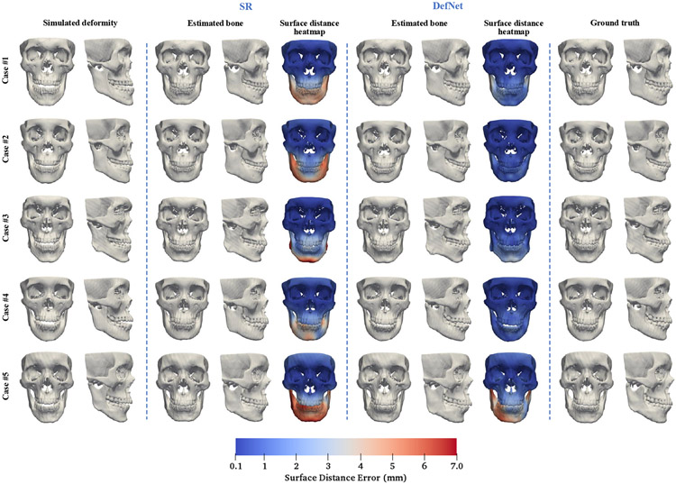
Figure 6 shows the simulated deformed bony surfaces, the estimated bony surfaces given by the methods, and the corresponding ground truth surfaces for five randomly selected testing cases. An experienced oral surgeon confirmed with visual assessment that our approach successfully restores normal shapes for various jaw deformities and yields comparable or better estimation performance than the SR method with lower surface distance errors.

Fig. 6.

Testing results for five random cases of synthetic data. The surface distance heatmaps are calculated by comparing positions of the corresponding vertices between the estimated and ground truth bony surfaces.

Since the goal is to restore the deformed jaw to its normal shape and keep the midface unchanged, we evaluated the estimation accuracy of the jaw and the midface separately. We calculated the four assessment metrics for the 1,598 testing cases, with quantitative results summarized in Table I (jaw) and Table II (midface). Table I indicates that there is no significant difference between the two competing methods in terms of VD, ED, SC, and LD for the jaw. This implies that our approach is comparable to the SR method for the jaw region. A similar conclusion can be drawn from Table II for the midface. In conclusion, DefNet achieves performance comparable to the SR method on the synthetic data.

TABLE I.

Statistics of VD (mm), ED (mm), SC, and LD (mm) for the Jaw Based on 1,598 Synthetic Patient Cases

	Method	Mean	SD	95% CI
VD	SR	3.60	1.26	(3.54, 3.66)
	DefNet	3.27	1.09	(3.22, 3.33)
ED	SR	0.25	0.07	(0.24, 0.25)
	DefNet	0.29	0.06	(0.29, 0.30)
SC	SR	0.72	0.06	(0.72, 0.73)
	DefNet	0.74	0.06	(0.74, 0.75)
LD	SR	3.63	0.97	(3.59, 3.68)
	DefNet	3.50	0.94	(3.45, 3.54)

SD: Standard deviation. CI: Confidence interval of the mean.

TABLE II.

Statistics of VD (mm), ED (mm), SC, and LD (mm) for the Midface Based on 1,598 Synthetic Patient Cases

	Method	Mean	SD	95% CI
VD	SR	0.49	0.21	(0.48, 0.50)
	DefNet	0.56	0.21	(0.55, 0.57)
ED	SR	0.07	0.03	(0.06, 0.07)
	DefNet	0.09	0.03	(0.08, 0.09)
SC	SR	0.99	0.01	(0.99, 1.00)
	DefNet	0.99	0.01	(0.99, 1.00)
LD	SR	0.00	0.00	(0.00, 0.00)
	DefNet	0.19	0.19	(0.18, 0.20)

SD: Standard deviation. CI: Confidence interval of the mean. The LD value given by the SR method is zero because the midface landmarks are fixed during simulation and correction.

E. Evaluation on Real Patient Data

To evaluate the proposed method on real clinical data, we collected paired pre-operative and post-operative head CT scans of another 24 patients with jaw deformities. The CT scans were segmented to extract the bony surfaces [22]. The post-operative bony surfaces served as the ground truth for evaluation. The post-operative bony surface was remeshed according to the pre-operative bony surface of the same patient (Fig. 7). Specially, we deformed the pre-operative bony surface onto the post-operative one based on the 51 surface landmarks. First, the post-operative surface was rigidly transformed to the pre-operative surface by matching their midface landmarks. Then, the full set of landmarks on the pre-operative and aligned post-operative bony surfaces were utilized to compute a deformation field via TPS interpolation [18]. The deformation field was subsequently applied on the pre-operative surface to generate the remeshed post-operative surface, which preserves the shape of the post-operative bone and maintains vertex-wise correspondences with the pre-operative surface. This allows us to evaluate estimation accuracy by computing the aforementioned assessment metrics.

Fig. 7.

Remeshing of the post-operative bony surface using the mesh topology of the corresponding pre-operative bony surface. The midface landmarks are in green and the jaw landmarks are in red.

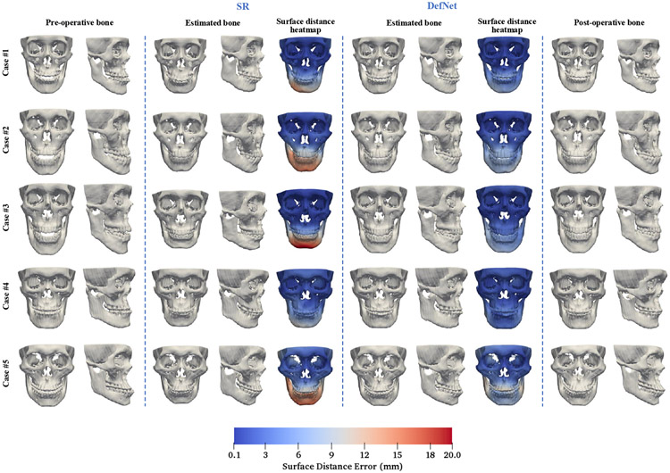
We trained the proposed deep learning model using the synthetic data and tested the trained model on the pre-operative bones of the 24 patients. The performance was evaluated by comparing the estimated bony surface with the corresponding post-operative bony surface. Results for the SR method are also included for comparison. Figure 8 shows the estimated bony surfaces and heatmaps of surface vertex distances for the two methods on five randomly selected cases. Based on visual inspection, an oral surgeon determined that all estimated reference models given by our method are clinically acceptable and are better than the ones achieved with the SR method. Table III shows that, for the jaw, VD and LD obtained by our approach are significantly smaller than the SR method (p < 0.05). Our method yields small improvements on ED and SC over the SR method. Table IV shows that, for the midface, the results are comparable between the two methods for the four metrics, implying similar capability in preserving the midface. Based on these results, we conclude that the proposed method outperforms the SR method on real patient data.

Fig. 8.

Corrected bony shapes estimated by the sparse representation method and DefNet for five random real patient cases.

TABLE III.

Statistics of VD (mm), ED (mm), SC, and LD (mm) for the Jaw Based on 24 Real Patient Cases

	Method	Mean	SD	Median	Min	Max
VD	SR	5.74	2.09	5.45	3.20	10.99
	DefNet	3.99	0.97	3.75	2.37	5.77
ED	SR	0.34	0.06	0.32	0.26	0.47
	DefNet	0.30	0.05	0.29	0.23	0.44
SC	SR	0.63	0.09	0.63	0.41	0.75
	DefNet	0.69	0.06	0.70	0.59	0.80
LD	SR	5.50	1.66	5.12	3.68	9.84
	DefNet	4.01	0.85	3.81	2.91	5.74

TABLE IV.

Statistics of VD (mm), ED (mm), SC, and LD (mm) for the Midface Based on 24 Real Patient Cases

	Method	Mean	SD	Median	Min	Max
VD	SR	1.32	0.38	1.22	0.80	2.08
	DefNet	1.33	0.37	1.28	0.67	2.00
ED	SR	0.15	0.04	0.14	0.08	0.23
	DefNet	0.15	0.04	0.15	0.10	0.21
SC	SR	0.96	0.04	0.97	0.88	1.00
	DefNet	0.95	0.04	0.96	0.87	1.00
LD	SR	1.29	0.43	1.23	0.72	2.01
	DefNet	1.30	0.43	1.25	0.71	2.02

F. Comparison with Alternative Point-Cloud Networks

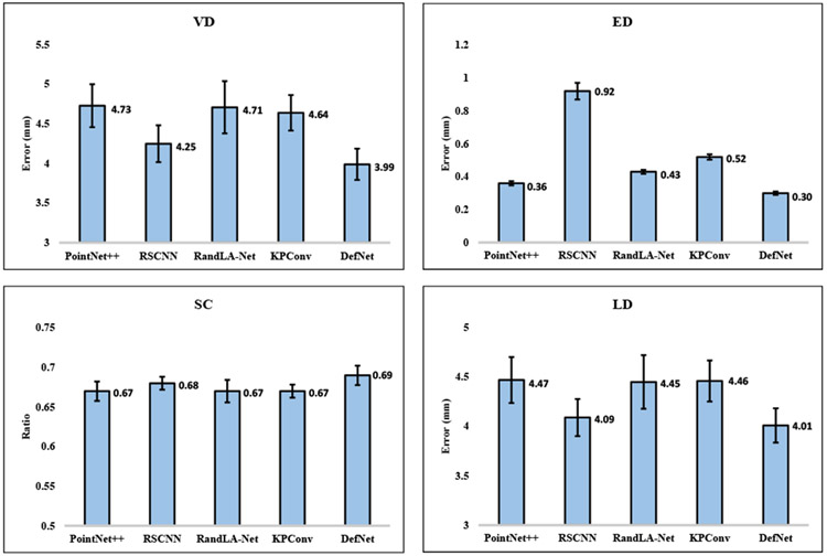
Our method leverages PointNet++ [11] and PointConv [17] for reference bony shape estimation. We compared our method with four other alternative point-cloud networks, i.e., the standard PointNet++, RSCNN [13], RandLA-Net [14], and KPConv [15]. We modified both the input and the output of the four alternative networks to match ours. We also replaced their loss functions with ours to match our task. With their default hyper-parameter settings, we trained the four networks using all paired synthetic data and tested the trained networks using the 24 pairs of pre-operative and post-operative patient bones. In Fig. 9, we compared the estimated bony surfaces produced by the five competing networks for two randomly selected patients. Based on visual inspection, an oral surgeon confirmed that the shape models estimated by our network are better than the other four networks. Quantitative evaluation results are shown in Fig. 10 (jaw) and Fig. 11 (midface). For the jaw, DefNet performs the best among the five competing networks and achieves significantly higher accuracy judging from the four metrics (p < 0.05). For the midface, DefNet, PointNet++, and RSCNN yield comparable performance (p > 0.05), but better performance than KPConv and RandLA-Net (p < 0.05).

Fig. 9.

Corrected bony shapes estimated by the standard PointNet++, RSCNN, RandLA-Net, KPConv, and DefNet for two real patient cases.

Fig. 10.

Performance comparison of the five networks for the jaw region based on 24 real patient cases.

Fig. 11.

Performance comparison of the five networks for the midface region based on 24 real patient cases.

G. Ablation Study

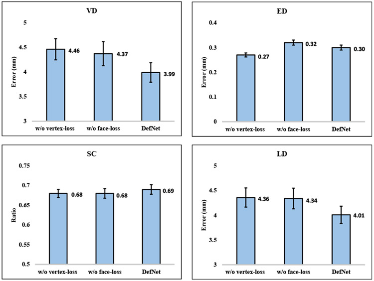
To verify the effectiveness of each component in the proposed loss design. We respectively trained DefNet without vertex-loss and without face-loss using the synthetic data, and tested the trained models on the 24 pairs of real patient data. The results, shown in Fig. 12 and Fig. 13, indicate that the full DefNet produces more accurate shape models, confirming the contribution of the two loss functions (i.e., L_vertex and L_face) in improving estimation.

Fig. 12.

Performance comparison between ablated networks and the full DefNet for the jaw region based on 24 real patient cases.

Fig. 13.

Performance comparison between ablated networks and the full DefNet for the midface region based on 24 real patient cases.

We evaluated DefNet with 6, 8, 10, and 12 convolutional layers with dimensions of point feature vectors as follows:

• {64, 128, 256, 256, 128, 128},

• {64, 128, 256, 512, 512, 256, 128, 128},

• {64, 128, 256, 512, 1024, 1024, 512, 256, 128, 128}, and

• {64, 128, 256, 512, 1024, 2048, 2048, 1024, 512, 256, 128, 128}.

For jaw estimation based on the 24 patients, Fig. 14 shows that DefNet with 8 and 10 layers yield comparable performance (p > 0.05) but significantly better performance than both 6 and 12 layers (p < 0.05). Figure 15 indicates that the four versions of DefNet are comparable in maintaining the midface (p > 0.05). The number of layers of DefNet was set to 8 to balance between accuracy and speed.

Fig. 14.

Medians of min-max normalized VD, ED, SC′ = 1 − SC, and LD for DefNet in jaw estimation.

Fig. 15.

Medians of min-max normalized VD, ED, SC′ = 1 − SC, and LD for DefNet in midface estimation.

H. Computational Cost

DefNet was implemented with Tensorflow [24] and trained on a 12 GB NVIDIA Titan Xp GPU. We trained the network for 200 epochs with an initial learning rate of 0.001. One epoch takes about 4 minutes and inference takes about 10 seconds.

IV. Discussion

In this paper, we applied geometric deep learning for orthognathic surgery planning by proposing a point-cloud network to estimate reference bony shape models. Compared with the sparse representation (SR) method [4], the proposed approach, DefNet, yields comparable performance for the synthetic data and better performance for the real data. The good performance of the SR method on the synthetic data is unsurprising because it was used to generate the training data for DefNet. However, the SR method generalizes poorly on the real data. In contrast, DefNet performs equally well on the real data due to its ability to learn deep point features. In addition, since DefNet takes as input point clouds consisting of vertices from surfaces, it is adaptable to 3D surfaces of varying topology. This is well suited for the facial bony surface, which can naturally be divided into two meshes (Fig. 16).

Fig. 16.

(a) A 3D facial bony surface divided into (b) “skull” and “mandible”.

Due to lack of ground truth reference bones, DefNet is trained on simulated pairs of deformed-normal bones. This strategy has proven to be effective judging based on the high estimation performance reported in Section III-E. However, since the simulated deformed bones are unlikely to cover all possible types of deformities, DefNet can potentially perform suboptimally when the deformity deviates significantly from simulation. A possible solution is to employ unsupervised learning with unpaired bony shapes without relying on simulated data.

V. Conclusion

We have developed a geometric deep learning framework for reference CMF bony shape estimation in orthognathic surgical planning. Experimental results confirm that we can train the network on synthetic data and then apply it to real patient data to obtain clinically acceptable reference bony shape models. Our method outperforms an existing sparse representation method, demonstrating that point-cloud deep learning is a more effective means for reference CMF bony shape estimation.

References

- [1].Xia JJ, Gateno J, and Teichgraeber JF, “Three-dimensional computer-aided surgical simulation for maxillofacial surgery,” Atlas Oral Maxillofac. Surg. Clin. North Am, vol. 13, no. 1, pp. 25–39, 2005. [DOI] [PubMed] [Google Scholar]
- [2].Xia JJ et al. , “Accuracy of the computer-aided surgical simulation (CASS) system in the treatment of patients with complex craniomaxillofacial deformity: A pilot study,” J. Oral Maxillofac. Surg, vol. 65, no. 2, pp. 248–254, 2007. [DOI] [PubMed] [Google Scholar]
- [3].Xia JJ et al. , “Algorithm for planning a double-jaw orthognathic surgery using a computer-aided surgical simulation (CASS) protocol. Part 1: planning sequence,” Int. J. Oral Maxillofacial Surg, vol. 44, no. 12, pp. 1431–1440, 2015. [DOI] [PMC free article] [PubMed] [Google Scholar]
- [4].Wang L et al. , “Estimating patient-specific and anatomically correct reference model for craniomaxillofacial deformity via sparse representation,” Med. Phys, vol. 42, no. 10, pp. 5809–5816, 2015. [DOI] [PMC free article] [PubMed] [Google Scholar]
- [5].Xiao Y, Lai Y, Zhang F, Li C, and Gao L, “A survey on deep geometry learning: From a representation perspective,” Comput. Vis. Media, vol. 6, no. 2, pp. 113–133, 2020. [Google Scholar]
- [6].Wu Z, Pan S, Chen F, Long G, Zhang C, and Yu PS, “A comprehensive survey on graph neural networks,” IEEE Trans. Neural Netw. Learn. Syst, 2020. DOI: 10.1109/TNNLS.2020.2978386. [DOI] [PubMed] [Google Scholar]
- [7].Defferrard M, Bresson X, and Vandergheynst P, “Convolutional neural networks on graphs with fast localized spectral filtering,” in Proc. Adv. Neural Inf. Process. Syst, 2016, pp. 3844–3852. [Google Scholar]
- [8].Kipf TN and Welling M, “Semi-supervised classification with graph convolutional networks,” in Proc. Int. Conf Learn. Representations, 2017, pp. 1–14. [Google Scholar]
- [9].Monti F, Boscaini D, Masci J, Rodola E, Svoboda J, and Bronstein MM, “Geometric deep learning on graphs and manifolds using mixture model CNNs,” in Proc. IEEE Conf. Comput. Vis. Pattern Recognit., 2017, pp. 5115–5124. [Google Scholar]
- [10].Charles RQ, Su H, Kaichun M, and Guibas LJ, “PointNet: Deep learning on point sets for 3D classification and segmentation,” in Proc. IEEE Conf. Comput. Vis. Pattern Recognit., 2017, pp. 652–660. [Google Scholar]
- [11].Qi CR, Yi L, Su H, and Guibas LJ, “PointNet++: Deep hierarchical feature learning on point sets in a metric space,” in Proc. Adv. Neural Inf. Process. Syst, 2017, pp. 5099–5108. [Google Scholar]
- [12].Guo Y, Wang H, Hu Q, Liu H, Liu L, and Bennamoun M, “Deep learning for 3D point clouds: A survey,” IEEE Trans. Pattern Anal. Mach. Intell, 2020. DOI: 10.1109/TPAMI.2020.3005434. [DOI] [PubMed] [Google Scholar]
- [13].Liu Y, Fan B, Xiang S, and Pan C, “Relation-shape convolutional neural network for point cloud analysis,” in Proc. IEEE Conf. Comput. Vis. Pattern Recognit., 2019, pp. 8895–8904. [Google Scholar]
- [14].Hu Q et al. , “RandLA-Net: Efficient semantic segmentation of large-scale point clouds,” in Proc. IEEE Conf. Comput. Vis. Pattern Recognit., 2020, pp. 11108–11117. [Google Scholar]
- [15].Thomas H, Qi CR, Deschaud JE, Marcotegui B, Goulette F, and Guibas LJ, “KPConv: Flexible and deformable convolution for point clouds,” in Proc. IEEE Int. Conf. Comput. Vis., 2019, pp. 6411–6420. [Google Scholar]
- [16].Turlach BA, “Bandwidth selection in kernel density estimation: A review,” Discussion Paper 9317, Inst. Statistique, B-1348 LouvainlaNeuve, Belgium, 1993. [Google Scholar]
- [17].Wu W, Qi Z, and Fuxin L, “PointConv: Deep convolutional networks on 3D point clouds,” in Proc. IEEE Conf. Comput. Vis. Pattern Recognit., 2019, pp. 9621–9630. [Google Scholar]
- [18].Bookstein FL, “Principal warps: Thin-plate splines and the decomposition of deformations,” IEEE Trans. Pattern Anal. Mach. Intell, vol. 11, no. 6, pp. 567–585, 1989. [Google Scholar]
- [19].Garland M and Heckbert P, “Surface simplification using quadric error metrics,” in Proc. SIGGRAPH 97, 1997, pp. 209–216. [Google Scholar]
- [20].Kingma D and Ba J, “Adam: A method for stochastic optimization,” in Proc. Int. Conf. Learn. Representations, 2015. pp. 1–41. [Google Scholar]
- [21].Yan J et al. , “Three-dimensional CT measurement for the craniomaxillofacial structure of normal occlusion adults in Jiangsu, Zhejiang and Shanghai Area,” China J. Oral Maxillofac. Surg, vol. 8, pp. 2–9, 2010. [Google Scholar]
- [22].Wang L et al. , “Automated segmentation of dental CBCT image with prior-guided sequential random forests,” Med. Phys, vol. 43, no. 1, pp. 336–346, 2016. [DOI] [PMC free article] [PubMed] [Google Scholar]
- [23].Lorensen WE and Cline HE, “Marching cubes: A high resolution 3D surface construction algorithm,” ACM SIGGRAPH Computer Graphics, vol. 21, no. 4, pp. 163–169, 1987. [Google Scholar]
- [24].Abadi M et al. , “TensorFlow: A system for large-scale machine learning,” in Proc. USENIX Symp. Oper. Syst. Design Implement, 2016, pp. 265–283. [Google Scholar]