Mixed-Effect Time-Varying Network Model and Application in Brain Connectivity Analysis

Abstract

Time-varying networks are fast emerging in a wide range of scientific and business applications. Most existing dynamic network models are limited to a single-subject and discrete-time setting. In this article, we propose a mixed-effect network model that characterizes the continuous time-varying behavior of the network at the population level, meanwhile taking into account both the individual subject variability as well as the prior module information. We develop a multistep optimization procedure for a constrained likelihood estimation and derive the associated asymptotic properties. We demonstrate the effectiveness of our method through both simulations and an application to a study of brain development in youth. Supplementary materials for this article are available online.

1. Introduction

The study of networks has recently attracted enormous attention, as they provide a natural characterization of many complex social, physical, and biological systems. A variety of statistical models have been developed to analyze network data; see Kolaczyk (2009) and Kolaczyk (2017) for a review. To date, much network research, however, has focused on static networks, where a single snapshot of the network is observed and modeled. Dynamic networks, where the data consist of a sequence of snapshots of the network that evolves over time, are fast emerging. Examples include brain connectivity networks, gene regulatory networks, protein signaling networks, and terrorist networks. Modeling of dynamic networks has appeared only recently, and most of those solutions considered a single-subject and discrete-time setting, in which the observed network is based upon the same study subject, and the observations are made on a finite and typically small number of discrete time points. Methodology for modeling dynamic networks in a multiple-subject and continuous-time setting remains largely missing. In this article, we develop a new network model to address this question.

Our motivation is a study of brain development in youth based on functional magnetic resonance imaging (fMRI). There has recently been increasing attention in understanding how brain functional connectivity develops during youth (Fair et al. 2009; Supekar, Musen, and Menon 2009). Brain connectivity reveals synchronization of brain systems via correlations in neurophysiological measures of brain activity, and when measured during resting state, it maps the intrinsic functional architecture of the brain (Varoquaux and Craddock 2013). Brain connectivity is commonly encoded by a network, and network analysis has become a crucial tool in understanding brain functional connectivity. Our data consist of 491 healthy young subjects. Their age ranges between 7 and 20 years, and was continuously measured. Each subject received a resting-state fMRI scan, and the image was preprocessed and summarized in the form of a network. The nodes of the network correspond to 264 seed regions of interest in brain (Power et al. 2011), and the links of the network record partial correlations between pairs of those 264 nodes. Partial correlation has been frequently employed to characterize functional connectivity among brain regions (Wang et al. 2016; Xia and Li 2017). Moreover, those 264 nodes have been partitioned into 10 functional modules that correspond to the major resting-state networks (Smith et al. 2009). Each module possesses a relatively autonomous functionality, and complex brain tasks are carried out through coordinated collaborations among those modules. The goal of this study is to investigate how functional connectivity at the whole-brain level varies with age, and in turn to understand how brain develops from childhood to adolescence and then to early adulthood.

To achieve this goal, we propose a new mixed-effect time-varying stochastic blockmodel. The brain functional module information naturally leads to our choice of blockmodel, as each functional module can be treated as a block in the blockmodel. Stochastic blockmodels have been intensively studied in the networks literature; see the review by Zhao (2017) and references therein. There have been some recent extensions to dynamic stochastic blockmodels (Xu and Hero 2014; Matias and Miele 2017; Zhang and Cao 2017). However, those solutions have been specifically designed for settings where the networks were observed for a single subject at a small number of time points. As such they are not directly applicable to our data problem, which involves multiple subjects and a continuously measured time variable. There is another family of statistical network models built upon sparse inverse covariance estimation (e.g., Friedman, Hastie, and Tibshirani 2008; Cai, Liu, and Luo 2011), but they usually target a static network and thus are different from our method. Notably, a recent proposal in this family by Qiu et al. (2016) can partially address our problem of modeling network dynamics over time. Specifically, Qiu et al. (2016) first obtained a covariance estimate at each observed age, and used kernel smoothing to estimate the covariance at any age in between. They then plugged the estimated covariance into a sparse inverse estimator such as the clime method of Cai, Liu, and Luo (2011). On the other hand, we note that Qiu et al. (2016) did not explicitly take into account the subject variability, and was not designed to incorporate the structure of functional modules either. Nevertheless, we compare with Qiu et al. (2016) numerically in both our simulations and real data analysis.

Our new model characterizes the dynamic behavior of the network at the population level through the fixed-effect term, and accounts for the subject-specific variability through the random-effect term. It works for the continuous-time setting, by modeling the connecting probabilities as functions of the time variable. It also naturally incorporates the module information available a priori. These features distinguish our proposal from most of the existing network models. Based on this model, we further introduce a shape constraint and a fusion constraint to regularize and improve our model estimation and interpretation. Both our model choice and the regularization constraints are guided and supported by current neurological findings, as well as evidences from the analysis of the motivating brain development data. The resulting model offers a good balance between model complexity and model flexibility, and is highly interpretable. We develop a multistep optimization procedure to estimate the unknown parameters in the proposed model, and derive the associated asymptotic properties with the diverging number of subjects. We further consider several extensions, including the case with diverging network size and the number of communities, the solution without shape constraint, and the setting with unknown community membership.

The contributions of our work are two-fold. Methodologically, the proposed model is able to characterize the time-varying nature of the network, account for the individual variability, and handle both the multisubject and continuous-time settings. It thus fills a gap in the existing literature on stochastic blockmodels, and makes a useful addition to the general toolbox of network modeling. Scientifically, we provide a systematic approach to model the increasingly available multisubject time-varying networks, and address a class of problems of immense scientific importance. We remark that, although motivated by a specific brain development study, our method is not limited to this application alone, but is applicable to a range of network problems. For instance, recent advances in single-cell sequencing technology are rapidly changing the landscape of gene expression data, and have the potential to characterize gene-gene regulatory networks underpinning changes in cellular state (Fiers et al. 2018). A growing number of methods have been proposed to infer gene networks based on single-cell sequencing data. One example is the human embryonic stem cell development study of Chu et al. (2016), which profiled 8700 genes in 758 single-cell samples at numerous time points of differentiation. A gene-gene network is constructed for each cell sample (Dai et al. 2019), and genes are grouped into different gene functional modules (Wang et al. 2015). Of scientific interest is to infer how the gene networks and how the interactions among different gene functional modules vary over time, and our method can be applied to address this problem.

The rest of the article is organized as follows. Section 2 develops the mixed-effect time-varying stochastic blockmodel and introduces the shape and fusion structures on the model parameters. Section 3 describes a multistep procedure for model estimation, and Section 4 investigates the associated asymptotic properties. Section 5 considers several extensions. Section 6 studies the empirical performance through simulations, and Section 7 analyzes the motivating brain development data.

2. Model

Suppose there are N subjects, ordered by a continuous time variable. Without loss of generality, we assume the time variable is sorted and normalized in that $0=r_1\le r_2\le \cdots \le r_{N-1}\le r_N=1$. In our example, the time variable is age, while it can represent other variable that orders the subjects as well. For each subject $i=1,\dots ,N$, a network ${\mathcal{G}}_i\left({\mathcal{V}}_i,{\mathcal{E}}_i\right)$ is observed, where ${\mathcal{V}}_i$ denotes the set of nodes and ${\mathcal{E}}_i$ the set of edges. Here we consider simple networks that are undirected and have no self-loops or multiple edges. Most real world networks, including brain connectivity networks, belong to this class. We also assume that all subjects share the same set of nodes, that is, ${\mathcal{V}}_1=\cdots ={\mathcal{V}}_N=\mathcal{V}$, and the size of $\mathcal{V}$ is n. This assumption is reasonable in our context, as brain images of different subjects are generally mapped to a common reference space. Each network ${\mathcal{G}}_i$ is uniquely represented by its n × n adjacency matrix A_i, where $A_{ij{j}^{\prime }}=1$ if there is an edge between nodes j and j′ for subject i, and $A_{ij{j}^{\prime }}=0$ otherwise,$1\le j\le j^{\prime }\le n$.

We adopt the stochastic blockmodel, in which the nodes are divided into blocks, or communities, and the probability of an edge between two nodes only depends on which communities they are in and is independent across edges given the community assignment. Specifically, we assume the nodes in $\mathcal{V}$ belong to K communities, and denote the community membership of node j as $c_j\in \left\{1,2,\dots ,K\right\}$, $j=1,\dots ,n$. We model the entries of the adjacency matrix A_i of subject i as independent Bernoulli random variables such that

$$\begin{gathered} \hspace{1em}\hspace{1em}{A}_{ij{j}^{\prime }}|r_i=t,c_j=k,c_{j^{\prime }}=l~\text{Bernoulli}\left(P_{ikl}\right), \\ g\left(P_{ikl}\right)={\theta }_{kl}\left(t\right)+w_i,\hspace{1em}{w}_i~\text{Normal}\left\{0,\sigma {\left(t\right)}^2\right\}, \end{gathered}$$ (1)

for $i=1,\dots ,N$, $1\le j,j^{\prime }\le ,1\le k,l\le K$. In this model, θ_kl(t) is the continuous-time connectivity function that characterizes the population level between-community connectivity when k ≠ l, and the within-community connectivity when k = l. It is modeled as a function of time t and is treated as a fixed-effect term, as it is commonly shared by all subjects. In our investigation, θ_kl(t) is the primary object of interest. The term w_i, for subject i, is the random-effect that is introduced to account for the subject-specific variability. It is assumed to follow a normal distribution with zero mean. Its variance σ (t)² is also time-varying, which is supported by the existing literature that the subject level variability varies with age (Nomi et al. 2017). On the other hand, different communities are assumed to share a common variance function σ²(t). This is a reasonable tradeoff between model complexity and flexibility. It allows one to pool information from different communities to estimate the variance function. The function g(‧) is a known, monotonic, and invertible link function. We set g(‧) as the logit link, while other link functions such as the probit link can also be used. We make two additional remarks. First, if there are additional subject-specific covariates, it is straightforward to incorporate those covariates into our model. That is, letting x_i denote the vector of covariates from subject i, we simply modify (1) with $g\left(P_{ikl}\right)={\theta }_{kl}\left(t\right)+{\mathit{x}}_i^{\top }\mathit{\beta }+w_i$, where β is the vector of covariate coefficients. For simplicity, we skip the term ${\mathit{x}}_i^{\top }\mathit{\beta }$ in this article. Second, in our model formulation, we assume the network community information is known, and it does not change over time. This assumption is both plausible and useful scientifically. In brain connectivity analysis, brain regions (nodes) are frequently partitioned into a number of known functional modules (communities). These communities are functionally autonomous, and they jointly influence brain activities. Moreover, although the connectivity within and between the functional modules vary with age, the nodes constituting those modules remain stable over age (Betzel et al. 2014). Focusing on those brain functional modules also greatly facilitates the interpretation, particularly when the brain network changes over time. We call model (1) a mixed-effect time-varying stochastic blockmodel.

Next, we propose to model the time-varying components θ_kl(t) and σ (t) as piecewise constant functions. This assumption is desirable for several seasons. Scientifically, numerous studies have found that the development of brain undergoes a mix of periods of rapid growth and plateaus (Zielinski et al. 2010; Geng et al. 2017). Such a pattern can be adequately captured when θ_kl(t) is piecewise constant. Moreover, functions with a simple structure such as piecewise constant enables an easier and clearer interpretation than those involving curvatures. Methodologically, the piecewise constant structure allows one to pool together subjects of similar ages to better estimate the variance of the subject-specific random-effect term w_i, which would in turn lead to an improved estimation of the connecting probabilities. This characteristic is particularly useful, since the individual variability is typically large in brain development studies. Theoretically, we show in Section 4 that, even when the true connectivity function θ_kl(t) does not admit a piecewise constant form, estimating it with a piecewise constant structure with a diverging number of constant intervals would still achieve a reasonable estimation accuracy. We also comment that, even though both terms are modeled as piecewise constant functions, our model is designed for a continuous time variable, as θ_kl(t) and σ (t) are defined for any t ∈ (0, 1], and the number of constant intervals is large and can diverge to infinity.

Specifically, we partition (0, 1] into S intervals; that is, $\left(0,1\right]={\bigcup }_{s=1}^S\left(t_{s-1},t_s\right]$ for $0=t_0<t_1<\cdots <t_S=1$. One can either use equal-length intervals, or set each interval to contain the same number of subjects. In Sections 6 and 7, we show that our method is not overly sensitive to the number of intervals S, in that a similar estimate is obtained as long as S is within a reasonable range. Theoretically, we allow S to go to infinity along with the sample size N. This allows our piecewise constant approximation to better capture the time-varying pattern, even if it changes frequently. Following the above partition, we assume that the connectivity function between the communities k and l is constant in (t_s−1, t_s] and denote it as θ_kl,s, and the random-effect variance function is constant in (t_s−1, t_s] and denote it as ${\sigma }_s^2$, $s=1,\dots S$. For simplicity, we introduce the same partitions for all θ_kl(t) and σ (t). However, as we show later in Section 4, we do not assume the true θ_kl(t) and σ (t) have to have the same constant intervals. We also introduce different fusion regularization parameters so that the constant intervals could vary for different θ_kl(t). Next we define the vector ${\mathit{\theta }}_{kl}={\left({\theta }_{kl,1},\dots ,{\theta }_{kl,S}\right)}^{\top }\in {ℝ}^S$, $\mathit{\sigma }={\left({\sigma }_1,\dots ,{\sigma }_S\right)}^{\top }\in {ℝ}^S$, and the matrix $\mathbf{\Theta }=\left({\mathit{\theta }}_{11},\dots ,{\mathit{\theta }}_{1K},{\mathit{\theta }}_{22},\dots ,{\mathit{\theta }}_{2K},\dots ,{\mathit{\theta }}_{KK}\right)\in {\mathcal{R}}^{S\times K\left(K+1\right)/2}$. Furthermore, let ${\tau }_i={\sum }_{s=1}^{S}I\left(r_i\le t_s\right)$ denote the interval that contains subject i, where I(‧) is the indicator function. Write $\mathit{A}=\left\{{\mathit{A}}_1,\dots ,{\mathit{A}}_N\right\}$, and $\mathit{c}=\left\{c_1,\dots ,c_n\right\}$, where A_i is the adjacency matrix of subject i, $i=1,\dots ,N$, and c_j is the community membership of node j,$j=1,\dots ,n$. We aim to estimate the parameters of interest Θ and σ by minimizing the loss function,

$$\begin{gathered} \mathcal{L}\left(\mathbf{\Theta },\mathit{\sigma }|\mathit{c},\mathit{A}\right)=-\text{log}\left\{\prod _{i=1}^N\prod _{j=1}^n\prod _{j^{\prime }>j}^n{P}_{i{c}_j{c}_{j^{\prime }}}^{A_{ij{j}^{\prime }}}{\left(1-P_{i{c}_j{c}_{j^{\prime }}}\right)}^{\left(1-A_{ij{j}^{\prime }}\right)}\right\} \\ =-\sum _{i=1}^N\text{log}\left\{{\int }_{-\infty }^{\infty }\prod _{k=1}^K\prod _{l\ge K}^K\frac{{\left(e^{{\theta }_{kl,{\tau }_i}+w_i}\right)}^{n_{ikl}}}{{\left(1+e^{{\theta }_{kl,{\tau }_i}+w_i}\right)}^{n_{kl}}}\varphi \left(w_i,{\sigma }_{{\tau }_i}^2\right)\text{d}{w}_i\right\}, \end{gathered}$$ (2)

where $\varphi \left(\cdot ,\cdot \right)$ is the zero mean normal density function, $n_{ikl}={\sum }_{1\le j\le j^{\prime }}{A}_{ij{j}^{\prime }}I\left(c_j=k,c_{j^{\prime }}=l\right)$, $n_k={\sum }_{j=1}^{n}I\left(c_j=k\right)$, and $n_{kl}=n_k{n}_l$, $1\le k\le l\le K$, $i=1,\dots ,n$. Figure 1, the left panel, shows the estimated connecting probability g⁻¹(θ₈₉) between the 8th and 9th communities, executive control and frontoparietal right, in our brain development example, after minimizing the loss function (2). Details on minimization of (2) are given in Section 3.

Figure 1.

Estimated connecting probability between two functional modules, with the endpoints connected with red dashed lines. Left panel: The estimate obtained by minimizing the loss function in (2) with no constraint; middle panel: the estimate with the shape constraint; right panel: the estimate with both the shape constraint and the fusion constraint.

It is seen from the plot that the estimated connecting probability roughly follows an increasing trend along with age; however, it is not strictly monotonic, with small fluctuations from approximately 9 to 16 years old. Next we introduce a shape constraint to the loss function (2), in that θ_kl(t) follows a certain shaped trajectory, such as monotonically increasing, monotonically decreasing, unimodal, and inverse unimodal shape. This constraint is both to facilitate the interpretation, and is scientifically plausible, supported by current human brain development studies (e.g., Sowell et al. 2003). Toward that end, we impose that

$${\mathit{\theta }}_{kl}\in {\mathcal{U}}_{kl},\hspace{1em}1\le k\le l\le K,$$

where ${\mathcal{U}}_{kl}$ complies with one of the following shape constraints,

1. the monotonically increasing shape:

   $$\begin{gathered} {\mathcal{U}}_{kl}=\{{\mathit{\theta }}_{kl}\in {ℝ}^S:{\mathit{\theta }}_{kl,1}\le \cdots \le {\mathit{\theta }}_{kl,s_{kl}}\le {\mathit{\theta }}_{kl,s_{kl}+1}\le \cdots \le \\ {\mathit{\theta }}_{kl,S}\}, \end{gathered}$$
2. the monotonically decreasing shape:

   $$\begin{gathered} {\mathcal{U}}_{kl}=\{{\mathit{\theta }}_{kl}\in {ℝ}^S:{\mathit{\theta }}_{kl,1}\ge \cdots \ge {\mathit{\theta }}_{kl,s_{kl}}\ge {\mathit{\theta }}_{kl,s_{kl}+1}\ge \cdots \ge \\ {\mathit{\theta }}_{kl,S}\}, \end{gathered}$$
3. the unimodal shape:

   $$\begin{gathered} {\mathcal{U}}_{kl}=\{{\mathit{\theta }}_{kl}\in {ℝ}^S:{\mathit{\theta }}_{kl,1}\le \cdots \le {\mathit{\theta }}_{kl,s_{kl}}\ge {\mathit{\theta }}_{kl,s_{kl}+1}\ge \cdots \ge \\ {\mathit{\theta }}_{kl,S}\hspace{0.17em}\text{for}\hspace{0.17em}1\le s_{kl}\le S\}, \end{gathered}$$
4. the inverse unimodal shape:

   $$\begin{gathered} {\mathcal{U}}_{kl}=\{{\mathit{\theta }}_{kl}\in {ℝ}^S:{\mathit{\theta }}_{kl,1}\ge \cdots \ge {\mathit{\theta }}_{kl,s_{kl}}\le {\mathit{\theta }}_{kl,s_{kl}+1}\le \cdots \le \\ {\mathit{\theta }}_{kl,S}\hspace{0.17em}\text{for}\hspace{0.17em}1\le s_{kl}\le S\}. \end{gathered}$$

Figure 1, the middle panel, shows the estimated g⁻¹(θ₈₉) under the loss function (2) and the unimodal constraint. It is clearly seen that the connectivity increases with age.

It is also seen from the middle panel in Figure 1 that the estimated connectivity at adjacent time points are often very close, and there are relatively a small number of time points with a substantial change in magnitude. We thus further introduce a fusion type constraint to encourage sparsity in difference of the coefficients. Specifically, we consider

$$\begin{gathered} {\Vert \mathit{D}{\mathit{\theta }}_{kl}\Vert }_0\le b_{kl},\hspace{0.17em}\hspace{0.17em}1\le k\le l\le K,\hspace{0.17em}\text{where} \\ \mathit{D}=\left(\begin{array}{cccccc}-1& 1& 0& \cdots & 0& 0\\ 0& -1& 1& \cdots & 0& 0\\ ⋮& & & & & \\ 0& 0& 0& \cdots & -1& 1\end{array}\right)\in {ℝ}^{\left(S-1\right)\times S}, \end{gathered}$$

${\Vert \cdot \Vert }_0$ is the ℓ₀ norm and equals the number of nonzero elements, b_kl is the fusion parameter that takes a positive integer value and is set different for different θ_kl. This hard thresholding fusion constraint in effect yields b_kl groups of distinct values in θ_kl, and thus facilitates the model interpretation. Moreover, it is able to reduce the estimation error, as the fusion constraint fits well with the piecewise constant model assumption, and can effectively pool information from adjacent time intervals. We also comment that, we have chosen a hard thresholding regularization using an ℓ₀ norm, over a soft thresholding one such as the total variation regularization which uses an ℓ₁ norm. The latter can be viewed as a convex relaxation of the former. However, our loss function is nonconvex, which makes the convex relaxation on the penalty term less effective. In addition, the ℓ₁-penalized total variation solution could sometimes be suboptimal, in that it may achieve a slower rate of convergence; see Rinaldo (2009, Theorems 3.1 and 3.2). The hard thresholding approach provides an appealing alternative and has been commonly used in high-dimensional sparse models (Shen, Pan, and Zhu 2012; Zhu, Shen, and Pan 2014). Figure 1, the right panel, shows the estimated g⁻¹(θ₈₉) under the loss function (2) with both the unimodal constraint and the fusion constraint. It is seen that the connectivity between those two functional modules experiences notable changes when the age is around 9, 13, and 19 years. The resulting estimate is more interpretable than the one without any constraint. We next develop an optimization algorithm for model estimation.

3. Estimation

We aim at the constrained optimization problem,

$$\begin{gathered} {\text{minimize}}_{\mathbf{\Theta },\mathit{\sigma }}\mathcal{L}\left(\mathbf{\Theta },\mathit{\sigma }|\mathit{c},\mathit{A}\right),\hspace{1em}\text{such that}\hspace{0.17em}{\mathit{\theta }}_{kl}\in {\mathcal{U}}_{kl}, \\ \text{and}\hspace{0.17em}{\Vert \mathit{D}{\mathit{\theta }}_{kl}\Vert }_0\le b_{kl}. \end{gathered}$$ (3)

This is a nontrivial optimization problem. The log-likelihood loss is nonconvex and involves an integration term that cannot be evaluated directly. The constraints introduce another layer of complexity. Together they render many existing optimization algorithms and the subsequent asymptotic analysis intractable in our setting. We propose a three-step sequential estimation procedure, which helps simplify the optimization. Sequential optimization has been commonly employed in modern statistical learning and optimization problems (see, e.g., Li, Wang, and Carroll 2010; Ke, Fan, and Wu 2015; Yu et al. 2019). We first summarize our optimization procedure in Algorithm 1, then describe each step in detail.

In Step 1, we seek the minimizer of the loss function (2) without any constraint. We first write (2) as $\mathcal{L}\left(\mathbf{\Theta },\mathit{\sigma }|\mathit{c},\mathit{A}\right)=-{\sum }_{i=1}^N\text{log}\left\{f_i\left({\mathit{A}}_i|\mathit{c},{\mathbf{\Theta }}_{{\tau }_i,\cdot },{\sigma }_{{\tau }_i}\right)\right\}$, where Θ_s,· is the sth row of matrix Θ, $s=1\dots ,S$ and

$$\begin{gathered} f_i\left({\mathit{A}}_i|\mathit{c},{\mathbf{\Theta }}_{{\tau }_i,\cdot },{\sigma }_{{\tau }_i}\right) \\ ={\int }_{-\infty }^{+\infty }\prod _{k=1}^K\prod _{l\ge k}^K\frac{{\left(e^{{\theta }_{kl,{\tau }_i}+w_i}\right)}^{n_{ikl}}}{{\left(1+e^{{\theta }_{kl,{\tau }_i}+w_i}\right)}^{n_{kl}}}\varphi \left(w_i,{\sigma }_{{\tau }_i}^2\right)\text{d}{w}_i. \end{gathered}$$ (4)

It involves an integration that cannot be evaluated exactly, but instead can be approximated through the adaptive Gauss–Hermite numerical integration (Pinheiro and Bates 1995). That is, we approximate the integral $\int f\left(a\right)\varphi \left(a\right)\text{d}a$ as,

$$\int f\left(a\right)\varphi \left(a\right)\text{d}a\approx \sum _{b=1}^{B}f\left(a_b\right)u_b,$$

where B is the number of quadrature points used in the approximation, a_b and u_b are the adaptive quadrature nodes and weights (Pinheiro and Bates 1995). A reasonable value of B ensures a good approximation of the integral, and we further discuss the choice of B in parameter tuning later. Accordingly, we approximate $f_i\left({\mathit{A}}_i|\mathit{c},{\mathbf{\Theta }}_{{\tau }_i},{\sigma }_{{\tau }_i}\right)$ with

$$\begin{gathered} {\tilde{f}}_i\left({\mathit{A}}_i|\mathit{c},{\mathbf{\Theta }}_{{\tau }_i},{\sigma }_{{\tau }_i}\right) \\ =\sum _{b=1}^B{u}_b\left\{\prod _{k=1}^K\prod _{l\ge l}^K\frac{{\left(e^{{\theta }_{kl,{\tau }_i}+{\sigma }_{{\tau }_h}{a}_b}\right)}^{n_{ikl}}}{{\left(1+e^{{\theta }_{kl,{\tau }_i}+{\sigma }_{{\tau }_i}{a}_b}\right)}^{n_{kl}}}\right\}. \end{gathered}$$ (5)

We then seek the minimizer,

$$\begin{gathered} (\tilde{\mathbf{\Theta }},\widehat{\mathit{\sigma }})={\text{arg min}}_{\mathbf{\Theta },\mathit{\sigma }}\tilde{\mathcal{L}}\left(\mathbf{\Theta },\mathit{\sigma }|\mathit{A},\mathit{c}\right) \\ =-\sum _{i=1}^N\text{log}\left\{{\tilde{f}}_i\left({\mathit{A}}_i|\mathit{c},{\mathbf{\Theta }}_{{\tau }_i},{\sigma }_{{\tau }_i}\right)\right\}. \end{gathered}$$ (6)

We achieve this by updating Θ and σ in an alternating fashion. The block coordinate decent algorithm is used for such an update (Tseng 2001). This alternating procedure is guaranteed to converge (Bates and Watts 1988), though likely to a local minimum, due to the nonconvexity of the objective function. Multiple initializations are thus recommended. If additional subject covariates x are incorporated in the model, the corresponding coefficient β can be estimated with some straightforward modification to the algorithm. The complexity of estimating β is comparable to that of estimating the fixed-effect term in a generalized linear mixed model.

In Step 2, we add the shape constraint to the loss function in (2), by computing a projection of ${\tilde{\mathit{\theta }}}_{kl}$, the column of $\tilde{\mathbf{\Theta }}$, to the set of shape constrained sequences,

$$\begin{gathered} {\stackrel{\vee }{\mathit{\theta }}}_{kl}={\text{arg min}}_{v_1,\dots ,v_S}\sum _{s=1}^S{\left(v_s-{\tilde{\theta }}_{kl,s}\right)}^2,\hspace{0.17em}\hspace{0.17em}\text{such that} \\ \left(v_1,\dots ,v_S\right)\in {\mathcal{U}}_{kl}. \end{gathered}$$ (7)

That is, we find the vector ${\stackrel{\vee }{\mathit{\theta }}}_{kl}={\left({\stackrel{\vee }{\theta }}_{kl,1},\dots ,{\stackrel{\vee }{\theta }}_{kl,S}\right)}^{\top }$ such that it satisfies the shape constraint specified in ${\mathcal{U}}_{kl}$, meanwhile minimizing the sum of squared error with respect to ${\tilde{\mathit{\theta }}}_{kl}={\left({\tilde{\theta }}_{kl,1},\dots ,{\tilde{\theta }}_{kl,S}\right)}^{\top }$. For the unimodal shape constraint, we first find the mode of the sequence, by performing an isotonic regression for each possible candidate, then taking the one that yields the smallest sum of squared error as the estimated mode. Once we locate the mode, finding a unimodal sequence breaks into finding two monotonic sequences, one monotonically increasing before the mode and the other monotonically decreasing after the mode, and each can be achieved by an isotonic regression. The isotonic regression is carried out using an efficient linear algorithm, the pool adjacent violators algorithm (Barlow et al. 1972). For the inverse unimodal constraint, the estimation can be carried out similarly. For the monotonic shape constraint, we simply skip the mode finding step, and the rest of implementation is the same. The main computational cost of our estimation procedure arises almost entirely from the first step of unconstrained maximum likelihood estimation. The computational cost of the shape constrained estimation is almost negligible.

In Step 3, we add the fusion constraint to the shape constrained estimate ${\stackrel{\vee }{\mathit{\theta }}}_{kl}$, by seeking

$${\widehat{\mathit{\theta }}}_{kl}={\text{arg min}}_{v_1,\dots ,v_S}\sum _{s=1}^S{\left(v_s-{\stackrel{\vee }{\theta }}_{kl,s}\right)}^2,\hspace{0.17em}\hspace{0.17em}\text{such}\hspace{0.17em}\text{that}\hspace{0.17em}{\Vert \mathit{D}\mathit{v}\Vert }_0\le b_{kl},$$ (8)

where $\mathit{v}={\left(v_1,\dots ,v_S\right)}^{\top }$, and b_kl is the fusion tuning parameter. A common way to incorporate the fusion penalty is through soft thresholding, such as in fused lasso (Tibshirani et al. 2005), but we employ a hard thresholding approach. Specifically, for a vector $\mathit{v}={\left(v_1,\dots ,v_S\right)}^{\top }\in {ℝ}^S$ and a positive integer number b ≤ S, we first truncate the vector Dv, such that we keep the largest (b−1) entries in their absolute values, and set the rest to zero. This would in effect yield that there are b groups of distinct values in v. We then average the values of v within each of those b groups. We call this a fusion operator, and denote it by Fuse(v, b). As a simple illustration, let $\mathit{v}={\left(0.1,0.2,0.3,0.5,0.6\right)}^{\top }$ and b = 2. Then $\mathit{D}v={\left(0.1,0.1,0.2,0.1\right)}^{\top }$ and after truncation, we obtain ${\left(0,0,0.2,0\right)}^{\top }$. This in effect suggests that there are two groups in v, with the first three entries v₁, v₂, v₃ of v belong to one group, and the last two entries v₄, v₅ belong to the other. We then average the values of v in each group, and obtain that $\text{Fuse}\left(\mathit{v},b\right)={\left(0.2,0.2,0.2,0.55,0.55\right)}^{\top }$.

It is important to note that, the added fusion structure in the third step actually preserves the shape constraint from the second step, in that the estimator after applying the fusion constraint still belongs to the parameter space under the shape constraint.

Lemma 1. Let $\mathcal{U}$ comply with one of the following shape constraints on sequences $\mathit{v}\in {ℝ}^S$: monotonically increasing, monotonically decreasing, unimodal, or inverse unimodal. For any $\mathit{v}\in \mathcal{U}$ and $b\in {\mathbb{N}}^{+}$, we have $\text{Fuse}\left(\mathit{v},b\right)\in \mathcal{U}$.

It is also noteworthy that our problem is largely different from the standard fused lasso for linear regression (Tibshirani et al. 2005). Our model involves a loss function that is nonconvex and has an integration term that cannot be evaluated directly. It tackles network modeling under the continuous time setting, and also involves a time-varying random-effect term. In addition to the fusion constraint, our method also incorporates the shape constraint, and the input of the fusion constrained estimation is the output of the shape constrained step. All these factors make our problem utterly different and pose new challenges compared to the standard fused lasso. Moreover, unlike the soft thresholding regularization of the standard fused lasso, we employ the hard thresholding regularization to effectively control the number of change points.

Our proposed estimation procedure involves a number of tuning parameters, including the number of intervals S, the number of quadrature points B in the integral approximation, and the fusion penalty parameters b_kl. For S, in our numerical analysis in Sections 6 and 7, we have experimented with a number of different values and found our final estimate is not overly sensitive to the choice of S. For B, we have also experimented with a range of values between 1 and 25, which is often deemed sufficient to provide a good approximation to the numerical integration. The final estimates with B in this range are very close. As a greater B value implies a higher computational cost, we fix B = 5 in our subsequent analysis. For b_kl, we propose to use the following BIC criterion for tuning,

$$\text{BIC}=-2{\tilde{\mathcal{L}}}_{kl}\left({\widehat{\mathit{\theta }}}_{kl},\widehat{\mathit{\sigma }}|\mathit{A},\mathit{c}\right)+\text{log}N\times df\left({\widehat{\mathit{\theta }}}_{kl}\right),$$

where $df\left({\widehat{\mathit{\theta }}}_{kl}\right)$ is the degrees of freedom and is defined as the number of unique elements in the vector ${\widehat{\mathit{\theta }}}_{kl}$, and

$${\tilde{\mathcal{L}}}_{kl}\left({\widehat{\mathit{\theta }}}_{kl},\widehat{\mathit{\sigma }}|\mathit{A},\mathit{c}\right)=\sum _{i=1}^N\text{log}\left\{\sum _{b=1}^B{u}_b\frac{{\left(e^{{\theta }_{kl,{\tau }_i}+\sqrt{2}{\sigma }_{{\tau }_i}{a}_b}\right)}^{n_{ikl}}}{\left(1+{\left(e^{{\theta }_{kl,{\tau }_i}+\sqrt{2}{\sigma }_{{\tau }_i}{a}_b}\right)}^{n_{kl}}\right)}\right\}.$$

4. Theory

We next investigate the asymptotic properties of our proposed estimator. In brain connectivity analysis, the numbers of brain regions and functional modules are usually fixed. The same holds true for many other applications; for example, in single-cell based gene network analysis, attention is often concentrated on a subset of genes and gene functional modules only. Therefore, we begin our asymptotic analysis with the number of network vertices n and the number of communities K fixed, whereas the number of subjects N goes to infinity. This is different from the classical network asymptotic analysis with only a single subject but the number of vertices tending to infinity. We study the extension of n, K → ∞ in Section 5.1.

We first introduce some notations. For a function $v\left(t\right)\in L^2\left(\left[0,1\right]\right)$, we define its function ℓ_q norm as ${\Vert v\Vert }_q={\left({\int }_0^1{\left|v\left(t\right)\right|}^{q}dt\right)}^{1/q}$. For two sequences {a_n} and {b_n}, we write $a_n\prec b_n$ if $a_n/b_n\to 0$ and $a_n\succ b_n$ if $a_n/b_n\to \infty$ as n → ∞. We write $a_n\asymp b_n$ if $a_n\le c{b}_n$ and $a_n\ge c^{\prime }{b}_n$ for some positive constants c and c′. Let θ_kl(t) denote the true underlying function,$1\le k,l\le K$. We first assume that θ_kl(t) complies with one of the shape constraints, monotonically increasing, monotonically decreasing, unimodal, or inverse unimodal. Later in Section 5.2, we will relax this shape constraint. We also assume θ_kl(t) is piecewise constant. Let p_kl denote the true number of constant intervals in θ_kl(t), and $p={\text{max}}_{1\le k,l\le K}{p}_{kl}$. We write $\left(0,1\right]={\bigcup }_{j=1}^{p_{kl}}\left(t_{kl,j-1},t_{kl,j}\right]$, for $0=t_{kl,0}<t_{kl,1}<\cdots <t_{kl,p_{kl}}=1$, and

$${\theta }_{kl}\left(t\right)=\sum _{j=1}^{p_{kl}}{\theta }_{kl,j}I\left\{t\in \left(t_{kl,j-1},t_{kl,j}\right]\right\}.$$

We assume that $\left|t_{kl,j-1}-t_{kl,j}\right|\asymp p_{kl}^{-1}$ for $j=1,\dots ,p_{kl}$, and write ${\mathit{\theta }}_{kl}={\left({\theta }_{kl,1},\dots ,{\theta }_{kl,p_j}\right)}^{\top }\in {ℝ}^{p_j}$. Given a chosen number of intervals S, the vector-valued global minimizer ${\stackrel{\vee }{\mathit{\theta }}}_{kl}$ from (7), and the global minimizer ${\widehat{\mathit{\theta }}}_{kl}$ from (8), we define the corresponding function estimators as

$${\stackrel{\vee }{\theta }}_{kl}\left(t\right)=\sum _{s=1}^S{\stackrel{\vee }{\theta }}_{kl,s}I\left\{t\in \left(\frac{s-1}{S},\frac{s}{S}\right]\right\}\hspace{1em}\hspace{0.17em}\text{and}$$

$${\widehat{\theta }}_{kl}\left(t\right)=\sum _{s=1}^S{\widehat{\theta }}_{kl,s}I\left\{t\in \left(\frac{s-1}{S},\frac{s}{S}\right]\right\}.$$

We assume ${\tilde{\mathit{\theta }}}_{kl}$ and $\widehat{\mathit{\sigma }}$ obtained from the first step of optimization are the global minimizers of (6). Moreover, for notational simplicity, here we let all the intervals in our estimation procedure have equal length. The same theoretical properties can be derived when each interval is chosen to contain the same number of subjects, but the notation would become more complicated. We thus focus on the equal-length interval case in this section.

We next introduce a set of main regularity conditions, and give some additional technical conditions in the supplementary materials.

Assumption 1. Assume that the number of intervals S and the number of subjects N satisfy that S = O(N^1−α) for some 0 < α < 1.

This assumption allows the number of intervals S to diverge along with the sample size N at a certain rate. The condition α < 1 ensures there are enough number of samples in each interval to yield an unconstrained maximum likelihood estimator that is close to the truth.

Assumption 2. For the true function θ_kl(t), there exists a piecewise constant function ${\theta }_{kl}^{\text{'}}\left(t\right)$ defined on the intervals $\left(\left(s-1\right)/S,s/S\right]$, $s=1,\dots ,S$, such that ${\Vert {\theta }_{kl}\left(t\right)-{\theta }_{kl}^{\text{'}}\left(t\right)\Vert }_2^2\prec p\text{log}S/N$. This assumption assumes that the true piecewise constant function θ_kl(t) can be well approximated, in terms of ℓ₂ norm, by a piecewise constant function defined on the intervals $\left(\left(s-1\right)/S,s/S\right]$, $s=1,\dots ,S$. Such an assumption on the approximation error is commonly imposed in nonparametric methods, and is analogous to, for example, the B-spline basis approximation error assumption (Huang, Horowitz, and Wei 2010).

Assumption 3. Define the total variation of the true function θ_kl(t) as $V\left({\mathit{\theta }}_{kl}\right)={\text{max}}_{1\le j\le p}{\mathit{\theta }}_{kl,j}-{\text{min}}_{1\le j\le p}{\mathit{\theta }}_{kl,j}$. Assume that $V\left({\mathit{\theta }}_{kl}\right)<c_1$ for some positive constant c₁, and $p\prec S^{1/3}$.

This assumption requires the total variation V(θ_kl) to be bounded from above. This is to avoid the overall estimation risk to become excessive in the shape constrained regression, so to guarantee its performance. A similar condition is often imposed in the isotonic and unimodal regression (Zhang 2002; Chatterjee and Lafferty 2019). Moreover, we impose that the number of constant intervals in the true function can diverge but not too fast.

Assumption 4. Define the gaps in θ_kl(t) as ${\Delta }_{kl,j}=\left|{\theta }_{kl,j}-{\theta }_{kl,j-1}\right|$, $j=1,\dots ,p_{kl}$. Assume that ${\Delta }_{kl,j}\succ p\sqrt{\left(p\hspace{0.17em}\text{log}\hspace{0.17em}S\right)/N}$, and the tuning parameter $b_{kl}\ge 2p,\hspace{0.17em}1\le k,l\le K$.

This assumption places a lower bound on the gaps among sequential distinct values of θ_kl(t). This is analogous to the minimal signal condition of the sparse coefficients in high-dimensional regressions (Fan, Xue, and Zou 2014). It is needed in the fusion step to guarantee that the fused estimator would not incorrectly merge together two distinct groups of coefficients in the true signal. Moreover, the lower bound on the tuning parameter b_kl ensures that the fusion step would correctly recover all distinctive groups of coefficients. This is analogous to the condition on the tuning parameter in soft thresholding based fused lasso (Rinaldo 2009).

In summary, Assumptions 1 and 2 ensure the performance of the unconstrained maximum likelihood estimator. Assumption 3 is for the shape constrained estimator, and Assumption 4 is for the fusion constrained estimator. Furthermore, the technical condition (C4) in the supplementary materials ensures the identifiability of the unique minimizer. Next, we present the main theorem of our proposed estimator.

Theorem 1. Under Assumptions 1–3, and the technical condition (C4) in the supplementary materials, we have

$${\Vert {\stackrel{\vee }{\theta }}_{kl}\left(t\right)-{\theta }_{kl}\left(t\right)\Vert }_2^2=O_p\left(\frac{p\text{log}S}{N}\right).$$ (9)

Additionally, under Assumption 4, we have

$${\Vert {\widehat{\theta }}_{kl}\left(t\right)-{\theta }_{kl}\left(t\right)\Vert }_2\le {\Vert {\stackrel{\vee }{\theta }}_{kl}\left(t\right)-{\theta }_{kl}\left(t\right)\Vert }_2,$$ (10)

where the equality holds if and only if ${\stackrel{\vee }{\theta }}_{kl}\left(t\right)={\widehat{\theta }}_{kl}\left(t\right)$.

We next make some remarks about the derived error rate. First, when the true function θ_kl(t) is indeed piecewise constant, the error rate obtained in (9) for our estimator ${\widehat{\theta }}_{kl}\left(t\right)$ is analogous to the rate that is commonly seen in sparse regressions, which is in the form of sparsity × log(dimension)/(sample size) (Bühlmann and Van De Geer 2011). In our setup, p plays the role of the sparsity quantity, and S the role of the dimension. Second, when the true function θ_kl(t) is not piecewise constant, we work under a misspecified model. Since the number of intervals S is allowed to grow with the sample size N, the difference between the true function and the piecewise constant approximation tends to zero as S tends to infinity. In this case, the number of distinct values in the approximation function scales with S, and the corresponding error rate becomes O_p(S log S)/N. This is analogous to the error rate that is commonly seen in non-sparse regressions, which is in the form of dimension × log(dimension)/(sample size) (Bühlmann and Van De Geer 2011). Third, we briefly comment on the tightness of the derived error bound. The rate in N comes from the unconstrained estimation step, and it matches with the error rate of an M-estimator (Van der Vaart 2000). The rate in p matches with the minimax rate of estimation in regressions with piecewise constant signals (Gao, Han, and Zhang 2019). Thus the orders of N and p are expected to be tight, which is further supported by the simulation in Section S2.3. On the other hand, the logarithm term log S comes from the shape constrained estimation, where we have adopted a recently established theoretical result for the error bound of unimodal regressions (Chatterjee and Lafferty 2019). This order of log S may be further improved. In particular, Gao, Han, and Zhang (2019) established the minimax risk bound for unimodal piecewise constant regressions, which includes a log log S term. However, the techniques of Gao, Han, and Zhang (2019) cannot be directly applied to our problem, since we consider two different error objectives, namely, the minimax risk ${\text{inf}}_{{\widehat{\mathit{\theta }}}_{kl}}{\text{sup}}_{{\mathit{\theta }}_{kl}\in {\mathcal{U}}_{kl}}\mathbb{E}{\Vert {\widehat{\mathit{\theta }}}_{kl}-{\mathit{\theta }}_{kl}\Vert }_2$ and ${\Vert {\widehat{\mathit{\theta }}}_{kl}-{\mathit{\theta }}_{kl}\Vert }_2$, for some ${\mathit{\theta }}_{kl}\in {\mathcal{U}}_{kl}$ in our case. We leave the construction of a tight error bound as potential future research.

In addition to the estimation error, it is also of interest to identify the constant intervals in the true piecewise constant function θ_kl(t), that is, to identify the locations of the change-points of the function. A direct implication of Theorem 1 is that we can achieve an approximate change-point recovery, in terms of some distance metric (Lin et al. 2017). Specifically, for a piecewise constant function θ (t), let $\mathcal{C}\left(\theta \right)$ denote the set of change-points in θ (t). For the true connectivity function θ_kl(t), we have $\mathcal{C}\left({\theta }_{kl}\right)=\left\{t_{kl,1},\dots ,t_{kl,p}\right\}$. For two discrete sets $\mathcal{A}$ and $\mathcal{B}$, define the Hausdorff distance (Rockafellar and Wets 2009) as,

$$d_H\left(\mathcal{A},\mathcal{B}\right)=\text{max}\left\{d\left(\mathcal{A}|\mathcal{B}\right),d\left(\mathcal{B}|\mathcal{A}\right)\right\},\hspace{1em}\text{where}$$

$$d\left(\mathcal{A}|\mathcal{B}\right)=\underset{b\in \mathcal{B}}{\text{max}}\hspace{0.17em}\underset{a\in \mathcal{A}}{\text{min}}\left|a-b\right|.$$

This metric measures the maximum distance of an element in $\mathcal{B}$ to its closet element in $\mathcal{A}$. Next we state our result on the approximate change-point recovery.

Corollary 1. Under the conditions of Theorem 1, we have

$$d_H\left\{\mathcal{C}\left({\widehat{\theta }}_{kl}\right),\mathcal{C}\left({\theta }_{kl}\right)\right\}=O_P\left(\frac{1}{N^{1-\alpha }}\right),$$

where α is as defined in Assumption 1.

This corollary ensures that our estimated time-varying connectivity ${\widehat{\theta }}_{kl}\left(t\right)$ can approximately recover, in terms of the Hausdorff distance, the locations of all the true change-points in θ_kl(t). It is a consequence of Assumptions 1 and 4 and Theorem 1, and its proof is omitted.

5. Extensions

In this section, we study several useful extensions. First, we consider the case when the number of network vertices and the number of communities diverge with the sample size. Second, we consider the case where the time-varying network connectivity does not follow a shaped trajectory. We modify our estimation procedure accordingly, and develop the corresponding theory. Finally, we consider the case where the community labels of the nodes are unknown, and develop a variational EM estimation procedure.

5.1. Diverging Network and Community Size

Theorem 1 assumes that the number of subjects N tends to infinity, whereas the number of vertices n and the number of communities K remain fixed. This fits well with our setting, but is different from the classical network asymptotic analysis, where there is usually only a single subject, that is, N = 1, but the number of vertices n goes to infinity. In the next corollary, we extend our result to the diverging n and K scenario.

Corollary 2. Under the conditions of Theorem 1, we have

$${\Vert {\stackrel{\vee }{\theta }}_{kl}\left(t\right)-{\theta }_{kl}\left(t\right)\Vert }_2^2=O_p\left(\frac{p\text{log}S}{n_k{n}_{l}N}\right),$$

where n_k and n_l are the sizes of the communities k and l, respectively. Moreover, under Assumption 4, the inequality (10) in Theorem 1 continues to hold.

We allow n and K to diverge at the same time and at any rate, as long as Assumption 1 holds and K ≤ n. This is because the diverging N/S from Assumption 1 alone is sufficient to ensure a consistent estimator in each interval. When n_k or n_l also diverges, the estimator would have a faster rate of convergence. If furthermore the community sizes are balanced, that is, ${\text{min}}_k{n}_k\asymp {\text{max}}_k{n}_k$, we have that $n_k=O\left(n/K\right)$, $k=1,\dots ,K$. Then ${\Vert {\stackrel{\vee }{\theta }}_{kl}\left(t\right)-{\theta }_{kl}\left(t\right)\Vert }_2^2=O_p\left(\frac{K^2}{n^2}\times \frac{p\text{log}S}{N}\right)$. Thus, the estimation accuracy improves with a larger n and a smaller K, and when $K\prec n$. We also note that the condition on N in Assumption 1 is still required, even if K is fixed and n → ∞. In this case, the diverging n leads to a larger number of edges in estimating θ_kl(t). Meanwhile, the random-effect term is subject-specific, and to estimate its time-varying variance, N is still required to diverge at a faster rate compared to S.

In Corollary 2, we have considered a dense network setting, that is, the connecting probability remains constant as n → ∞. To control the sparsity of the network, a common approach is to reparameterize the connecting probability P_kl such that P_kl = ρ_nS_kl (Bickel and Chen 2009). After the reparameterization, the parameter S_kl remains constant in n, while ρ_n > 0 is a scalar such that ρ_n → 0 as n → ∞. In our setting, our parameter of interest θ_kl(t) is related to the connecting probability P_kl(t) through a logistic function. Adopting a similar approach to control the sparsity, we can reparametrize $P_{kl}\left(t\right)$ as $P_{kl}\left(t\right)={\rho }_n{e}^{{\theta }_{kl}\left(t\right)+w_i}/\left\{1+e^{{\theta }_{kl}\left(t\right)+w_i}\right\}$, with the positive scalar coefficient ρ_n → 0. If we further assume that ${\rho }_n\succ \text{log}n/n$, the result in Corollary 2 still holds. Its proof is almost identical to Theorem 1 and Corollary 2, and is thus omitted here. The condition ${\rho }_n\succ \text{log}n/n$ assumes that the network’s average degree grows faster than log n, and is a fairly common condition in the stochastic block model literature (Bickel and Chen 2009; Bickel et al. 2013).

5.2. No Shape Constraint

Motivated by the brain connectivity example, we have imposed the shape constraint in our estimation. Next we study the case where we impose no shape constraint. We still include the fusion constraint, so to account for the smoothness along the time variable.

The optimization problem (3) now becomes

$${\text{minimize}}_{\mathbf{\Theta },\mathit{\sigma }}\mathcal{L}\left(\mathbf{\Theta },\mathit{\sigma }|\mathit{c},\mathit{A}\right),\hspace{0.17em}\hspace{0.17em}\hspace{0.17em}\text{such}\hspace{0.17em}\text{that}\hspace{0.17em}\hspace{0.17em}{\Vert \mathit{D}{\mathit{\theta }}_{kl}\Vert }_0\le b_{kl}.$$ (11)

We modify Algorithm 1 to solve (11). Specifically, Step 1 remains the same, and Step 2 becomes a fusion constrained optimization,

$${\widehat{\mathit{\theta }}}_{kl}^{\ast }={\text{arg min}}_{v_1,\dots ,v_S}\sum _{s=1}^S{\left(v_s-{\tilde{\theta }}_{kl,s}\right)}^2,\hspace{0.17em}\hspace{0.17em}\text{such}\hspace{0.17em}\text{that}\hspace{0.17em}{\Vert \mathit{D}v\Vert }_0\le b_{kl}.$$ (12)

This step can be carried out using the Fuse(v, b) operator described in Section 3. Given a chosen number of intervals S and the minimizer ${\widehat{\mathit{\theta }}}_{kl}^{\ast }$ from (12), we define the corresponding function estimator as

$${\widehat{\theta }}_{kl}^{\ast }\left(t\right)=\sum _{s=1}^S{\widehat{\theta }}_{kl,s}^{\ast }I\left\{t\in \left(\frac{s-1}{S},\frac{s}{S}\right]\right\}.$$

We next establish its asymptotic properties. We modify Assumptions 3 and 4 accordingly.

Assumption 3*.$p\prec S$.

Assumption 4*. Denote the gaps in θ_kl(t) as ${\Delta }_{kl,j}=\left|{\theta }_{kl,j}-{\theta }_{kl,j-1}\right|$, $j=1,\dots ,p$. Assume that ${\Delta }_{kl,j}\succ p\sqrt{S/N}$, and the tuning parameter $b_{kl}\ge 2p$, $1\le k,l\le K$.

Since there is no shape constraint, the bound on the total variation in Assumption 3 is no longer needed. Correspondingly, we are able to relax the condition on p, since $p\times {\text{min}}_j{\Delta }_{kl,j}$ does not need to be upper bounded any more. On the other hand, the lower bound on ${\Delta }_{kl,j}$ in Assumption 4* that ${\Delta }_{kl,j}\succ p\sqrt{S/N}$ is stronger than that ${\Delta }_{kl,j}\succ p\sqrt{\left(p\hspace{0.17em}\text{log}\hspace{0.17em}S\right)/N}$ in Assumption 4, as p is of a smaller order than S. This stronger condition is also due to the removal of the shape constraint, since this constraint can potentially help reduce the error of the unconstrained estimator.

The next theorem then states the error rate of the estimator ${\widehat{\theta }}_{kl}^{\ast }\left(t\right)$ without the shape constraint, as well as its approximate change-point recovery property.

Theorem 2. Under Assumptions 1, 2, 3*, 4*, and the technical condition (C4) in the supplementary materials, we have

$${\Vert {\widehat{\theta }}_{kl}^{\ast }\left(t\right)-{\theta }_{kl}\left(t\right)\Vert }_2^2=O_p\left(\frac{p}{N}\right)\hspace{1em}\text{and}$$

$$d_H\left\{\mathcal{C}\left({\widehat{\theta }}_{kl}^{\ast }\right),\mathcal{C}\left({\theta }_{kl}\right)\right\}=O_p\left(\frac{1}{N^{1-\alpha }}\right).$$

Comparing Theorem 2 to Theorem 1, we see that the upper error bound of the estimator without the shape constraint is smaller by a log S term. However, we note that these two bounds are not directly comparable, since they are obtained under different conditions. We also note that, in the finite sample setting, the shape constraint helps improve the interpretability of the estimator, and often the estimation accuracy as well.

5.3. Unknown Network Community Membership

So far we assume that the community memberships of the nodes are known, since in brain connectivity analysis, we know which functional module each brain region belongs to. Next we study the extension where the network community memberships are unknown.

Specifically, suppose the community membership vector ${\left(c_1,\dots ,c_n\right)}^{\top }$, $c_j\in \left\{1,\dots ,K\right\}$, follows a multinomial distribution with the parameter vector $\mathit{\pi }=\left({\pi }_1,\dots ,{\pi }_K\right)$, but c is unobserved. Write $\mathit{w}={\left(w_1,\dots ,w_N\right)}^{\top }$. The loss function (2) becomes

$$\mathcal{L}\left(\mathbf{\Theta },\mathit{\sigma },\pi |\mathit{A}\right)=-\text{log}\left[\sum _{\mathit{c}\in {\left\{1,\dots ,K\right\}}^n}{\int }_{\mathit{w}}h\left(\mathit{A},\mathit{c},\mathit{w}|\text{Θ,}\mathit{\sigma },\mathit{\pi }\right)\text{d}\mathit{w}\right],$$ (13)

where

$$\begin{gathered} h\left(\mathit{A},\mathit{c},\mathit{w}|\text{Θ,}\mathit{\sigma },\mathit{\pi }\right) \\ =\prod _{j=1}^n{\mathit{\pi }}_{c_j}\prod _{i=1}^N\prod _{k=1}^K\prod _{l\ge k}^K\frac{{\left(e^{{\theta }_{kl,{\tau }_i}+w_i}\right)}^{n_{ikl}}}{{\left(1+e^{{\theta }_{kl,{\tau }_i}+w_i}\right)}^{n_{kl}}}\varphi \left(w_i,{\sigma }_{{\tau }_i}^2\right), \end{gathered}$$

and τ_i, n_ikl, and n_kl are the same as defined in (2). Maximizing (13) directly is computationally impractical, since it involves the summation over Kⁿ terms, which quickly becomes too large when n and K increase. Moreover, the conditional distribution of c on A, w, Θ, σ, π is complicated, rendering the standard expectation-maximization (EM) algorithm intractable. Alternatively, we consider a variational EM approach (Daudin, Picard, and Robin 2008), which aims at optimizing an upper bound of the loss function $\mathcal{L}\left(\mathbf{\Theta },\mathit{\sigma },\mathit{\pi }|\mathit{A}\right)$. That is, we consider

$$\begin{gathered} \mathcal{J}\left(\tilde{h};\mathbf{\Theta },\mathit{\sigma },\mathit{\pi }|\mathit{A}\right) \\ =-\text{log}{\int }_{\mathit{w}}\text{exp}[-\sum _{\mathit{c}}D\left\{\tilde{h}\Vert h\left(c|\mathit{A},\mathit{w},\text{Θ,}\mathit{\sigma },\mathit{\pi }\right)\right\} \\ +\text{log}h\left(\mathit{A},\mathit{w}|\text{Θ,}\mathit{\sigma },\mathit{\pi }\right)]\text{d}\mathit{w}, \end{gathered}$$

where $\tilde{h}$ is an approximation of $h\left(c|\mathit{A},\mathit{w},\text{Θ,}\mathit{\sigma },\mathit{\pi }\right)$, $D\left(\cdot \Vert \cdot \right)$ is the Kullback–Leibler divergence, and $h\left(\mathit{A},\mathit{w}|\text{Θ,}\mathit{\sigma },\mathit{\pi }\right)={\sum }_{\mathit{c}\in {\left\{1,\dots ,K\right\}}^n}h\left(\mathit{A},\mathit{c},\mathit{w}|\mathbf{\Theta },\mathit{\sigma },\mathit{\pi }\right)$. Note that $\mathcal{J}\left(\tilde{h};\text{Θ,}\mathit{\sigma },\mathit{\pi },\mathit{A}\right)$ is bounded below by the observed data loss function $\mathcal{L}\left(\text{Θ,}\mathit{\sigma },\mathit{\pi }|\mathit{A}\right)$, and this lower bound is reached only when $\tilde{h}=h\left(c|\mathit{A},\mathit{w},\text{Θ,}\mathit{\sigma },\mathit{\pi }\right)$. We limit $\tilde{h}$ to the class of completely factorized distributions, that is, $\tilde{h}\left(\mathit{c}\right)={\prod }_{i=1}^n{\tilde{h}}_i\left(c_i,{\mathit{\alpha }}_i\right)$, where ${\tilde{h}}_i$ denotes the multinomial distribution with the probability vector ${\mathit{\alpha }}_i={\left({\alpha }_{i1},\dots ,{\alpha }_{iK}\right)}^{\top }$. Based on the definition of Kullback–Leibler divergence, we can rewrite $\mathcal{J}\left(\tilde{h};\text{Θ,}\mathit{\sigma },\mathit{\pi },\mathit{A}\right)$ as,

$$\begin{gathered} \mathcal{J}\left(\tilde{h};{\left\{{\mathit{\alpha }}_i\right\}}_{i=1}^n\text{,Θ,}\mathit{\sigma },\mathit{\pi },\mathit{A}\right)=-\sum _{j=1}^n\sum _{k=1}^K{\alpha }_{jk}\text{log}\frac{{\pi }_k}{{\alpha }_{jk}} \\ -\sum _{i=1}^N\sum _{j\ne j^{\prime }}^n\sum _{k\ge l}^K{\alpha }_{jk}{\alpha }_{j^{\prime }l}{A}_{ij{j}^{\prime }}{\theta }_{kl,{\tau }_i}+\sum _{i=1}^N\text{log}\left(2\pi {\sigma }_{{\tau }_i}^2\right) \\ -\sum _{i=1}^N\text{log}\int \text{exp}(\sum _{j\ne j^{\prime }}^n\sum _{k\ge l}^K{\alpha }_{jk}{\alpha }_{j^{\prime }l}[A_{ij{j}^{\prime }}{w}_i \\ -\text{log}\left\{1+\text{exp}\left({\theta }_{kl,{\tau }_i}+w_i\right)\right\}]-\frac{w_i^2}{2{\sigma }_{{\tau }_i}^2})\text{d}{w}_i. \end{gathered}$$ (14)

Next, given a set of initial values ${\{{\mathit{\alpha }}_i^{\left(0\right)}\}}_{i=1}^n$, we maximize $\mathcal{J}\left(\tilde{h};{\left\{{\mathit{\alpha }}_i\right\}}_{i=1}^n,\mathbf{\Theta },\mathit{\sigma },\mathit{\pi },\mathit{A}\right)$ with respect to ${\left\{{\mathit{\alpha }}_i\right\}}_{i=1}^n$ and {Θ, σ, π }, iteratively. We summarize this new optimization procedure in Algorithm 2. The integral term in $\mathcal{J}$ is evaluated using the adaptive Gauss-Hermite numerical integration, similar to (5). In Step 1.1 of the algorithm, it requires an optimization over a high-dimensional parameter space {Θ, σ, π}. Its computational cost can be significantly reduced, by noting that $\mathcal{J}\left(\tilde{h};{\left\{{\mathit{\alpha }}_i^{\left(q\right)}\right\}}_{i=1}^n,\mathbf{\Theta },\mathit{\sigma },\mathit{\pi },\mathit{A}\right)$ can be factorized into separate objective components with respect to $\left\{{\mathbf{\Theta }}_{1,\cdot },{\sigma }_1\right\},\dots ,\left\{{\mathbf{\Theta }}_{S,\cdot },{\sigma }_S\right\}$ and π, respectively. In Step 1.2, we employ the fixed point algorithm of Daudin, Picard, and Robin (2008). Furthermore, we obtain the initial values ${\{{\mathit{\alpha }}_i^{\left(0\right)}\}}_{i=1}^n$ by applying a standard spectral clustering algorithm (Bickel et al. 2013) to ${\sum }_{i=1}^N{\mathit{A}}_i/N$. We select the number of communities K using the integrated classification likelihood criterion (Biernacki, Celeux, and Govaert 2000). In our simulations, we have observed that our variational EM algorithm often converges in fewer than 10 iterations.

In this work, we do not pursue the theory for the constrained variational EM estimator. It is very challenging to obtain the consistency and asymptotic normality of even the unconstrained variational EM estimator under our model formulation. Such an analysis warrants a full investigation and a separate paper, and we leave it as future research.

6. Simulations

Next we investigate the finite sample performance of our proposed method. We generate N subjects with the age variable simulated from a uniform distribution on [0, 1]. For each subject, a network is generated based on a stochastic blockmodel, with n nodes belonging to K communities. We first consider n = 75, K = 2, and the two communities have the number of nodes equal to n₁ = 50 and n₂ = 25, respectively. We consider different ways of generating the within-community and between-community connectivity functions {θ₁₁(t), θ₁₂(t), θ₂₂(t)} and the variance function of the random-effect σ²(t).

Example A:

The connectivity functions are time-varying, while the variance of the random-effect is fixed over time. Specifically, we set logit⁻¹{θ₁₁(t)} and logit⁻¹{θ₂₂(t)} to take the functional form as shown in the first panel, and logit⁻¹{θ₁₂(t)} as shown in the second panel of Figure 2. In this setting, the within-community and between-community time-varying connecting probability follow different trajectories. The within-community connecting probability is monotonically increasing with [0, 0.2], (0.2, 0.5], (0.5, 0.7], and (0.7, 1] as true intervals, whereas the between-community connecting probability is monotonically decreasing with [0, 0.3], (0.3, 0.5], (0.5, 0.8], (0.8, 1] as the true intervals. We set σ = 0.1.

Figure 2.

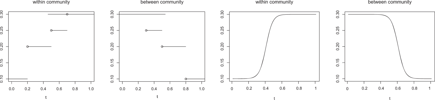
Two scenarios of the true within-community and between-community connecting probabilities as functions of time.

Example B:

Both the connectivity functions and the variance function are time-varying. Specifically, we choose the same {θ₁₁(t), θ₁₂(t), θ₂₂(t)} as in Example A, and set σ (t) = 0.2 − 0.1I(t > 0.5). This is motivated by the scientific finding that there is usually a higher variability in functional connectivity when subjects are at a younger age (Nomi et al. 2017).

Example C:

Both the connectivity functions and the variance function are time-varying. Moreover, the connectivity functions are no longer piecewise constant, but instead continuous functions. This example thus evaluates the performance of our method under model misspecification. Specifically, we set logit⁻¹ {θ₁₁(t)} and logit−1 {θ₂₂(t)} to take the functional form as shown in the third panel, and logit⁻¹ {θ₁₂(t)} as shown in the fourth panel of Figure 2. In this setting, the within-community connectivity is monotonically increasing and goes through a continuous and notable increase between t = 0.2 and t = 0.6; the between-community connectivity is monotonically decreasing and goes through a continuous decrease between t = 0.4 and t = 0.8. We again set σ (t) = 0.2 − 0.1I(t > 0.5).

We compare four estimation methods. The first is the proposed shape and fusion constrained estimator from Algorithm 1. The second is the unconstrained estimator from (6). The third is the fusion constrained estimator from (12). The fourth is the cubic B-spline estimator obtained from fitting B-splines to the estimated single-subject stochastic blockmodel. Specifically, for each subject i, we estimate the within and between-community connecting probability ${\widehat{P}}_{ikl}$, $1\le k\le l\le n$ based on the observed network A_i and the community label c. Here we assume c is known, and investigate the unknown c case later. We then order the estimated ${\widehat{P}}_{ikl}$‘s by the subject’s age and obtain the B-spline estimator using spline regression, with S − 1 interior knots equally spaced in [0, 1]. In our implementation, we use S equal-length intervals for the first three methods. Since the age variable is generated from a uniform distribution, choosing the intervals to have the same length or to contain the same number of subjects lead to essentially the same results for this example. Furthermore, we employ the unimodal shape constraint in the first method, and use BIC to tune the fusion penalty parameters. The estimation error is evaluated based on the criterion,

$${\left[\frac{2}{K\left(K+1\right)}\sum _{k\le l}^K{\int }_0^1{\left\{{\widehat{\theta }}_{kl}\left(t\right)-{\theta }_{kl}\left(t\right)\right\}}^2\text{d}t\right]}^{1/2},$$ (15)

where ${\widehat{\theta }}_{kl}\left(t\right)$ is the estimated θ_kl(t).

Figure 3 reports the results based on 50 data replications, with the sample size fixed at N = 1000. For Example A (the left panel), we observe that our proposed shape and fusion constrained estimator achieves the best overall performance, as long as the number of intervals S is reasonably large (S ≥ 10). Moreover, its performance is stable for a wide range of values of S. This is an appealing feature of our estimator. By contrast, the unconstrained estimator is much more sensitive to the choice of S. This is because it does not borrow information across different time intervals as the constrained estimator does. The fusion constrained estimator achieves a similar performance as the shape and fusion constrained estimator when S is in a reasonable range (S < 100), but it performs worse when S is large (S ≥ 100). Additionally, the spline estimator performs poorly, since the underlying true function is piecewise constant rather than smooth. For Example B (the middle panel), we again observe that our proposed shape and fusion constrained estimator performs the best, and remains relatively stable across a wide range of values of S. As a comparison, both the unconstrained and the fusion constrained estimators perform worse when the random-effect variance varies over time. The spline estimator continues to perform poorly in this setting. For Example C (the right panel), we see that, when S < 10, the spline estimator achieves a smaller estimation error, but when S > 10, it yields a larger estimation error due to overfitting. By contrast, our proposed shape and fusion constrained estimator maintains a competitive performance, even though the underlying true functions are continuous and our model is misspecified. Moreover, both the unconstrained and the fusion constrained estimators perform poorly. This example suggests that, in the finite sample setting, the shape constraint can help improve the estimation accuracy.

Figure 3.

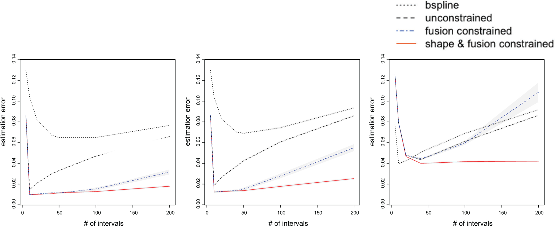
Estimation error of four different methods: the proposed shape and fusion constrained estimator (solid red line), the unconstrained estimator (black dashed line), the fusion constrained estimator (blue dashed line), and the cubic B-spline estimator (black dotted line). The gray bands are the 95% confidence interval.

We also vary the sample size N = 200, 1000 for different values of S = 20, 50 in the above examples. Table 1 reports the average estimation error and the standard error (in parenthesis) for the four methods based on 50 data replications. For Examples A and B, it is seen that the performance of the proposed shape and fusion constrained estimator achieves the best performance, and it improves with a larger sample size N and a smaller number of intervals S. This observation agrees with our theoretical results. When N = 200, the shape and fusion constrained estimator performs better for S = 20 than for S = 50. This is because, when N is limited and S is large, there are too few subjects per interval, which leads to a poor estimation in the first step. However, when N = 1000, the proposed estimator performs similarly when S = 20 and S = 50, since now there are enough number of subjects per interval. In general, we recommend a reasonable range for S so that there are roughly at least 10 subjects per interval.

Table 1.

Average estimation errors (with standard errors in the parenthesis) of four methods with varying sample size N and number of intervals S.

Method	N	Example A		Example B		Example C
		S = 20	S = 50	S = 20	S = 50	S = 20	S = 50
Shape and fusion constraint	200	0.0319 (0.0012)	0.0469 (0.0012)	0.0352 (0.0012)	0.0562 (0.0013)	0.0662 (0.0010)	0.0686 (0.0010)
	1000	0.0103 (0.0003)	0.0114 (0.0004)	0.0133 (0.005)	0.0150 (0.0007)	0.0460 (0.0002)	0.0389 (0.0004)
Fusion constraint	200	0.0339 (0.0013)	0.0589 (0.0016)	0.0390 (0.0015)	0.0770 (0.0017)	0.0703 (0.0011)	0.0893 (0.0011)
	1000	0.0103 (0.0003)	0.0113 (0.0004)	0.0131 (0.0005)	0.0150 (0.0006)	0.0472 (0.0003)	0.0456 (0.0004)
No constraint	200	0.0509 (0.0009)	0.0794 (0.0008)	0.0614 (0.0010)	0.0982 (0.0012)	0.0729 (0.0010)	0.0980 (0.0011)
	1000	0.0208 (0.0004)	0.0329 (0.0003)	0.0279 (0.0005)	0.0431 (0.0005)	0.0482 (0.0004)	0.0462 (0.0004)
Cubic B-spline	200	0.0946 (0.0005)	0.0958 (0.008)	0.1013 (0.0008)	0.1108 (0.0011)	0.0718 (0.0011)	0.1037 (0.0011)
	1000	0.0821 (0.0002)	0.0646 (0.0002)	0.0832 (0.0002)	0.0688 (0.0003)	0.0411 (0.0004)	0.0531 (0.0005)

We have also run simulations with different network size n and the number of communities K, and investigate the effect of the within and between-community connectivity difference and network density on the estimation. In addition, we run a simulation with the unknown community membership c. We also numerically compare with a simple baseline method and Qiu et al. (2016). In the interest of space, we report these additional results in the supplementary materials.

Computationally, we find our proposed method runs fast. For instance, for Example C with N = 200, one simulation run took on average 3.81 sec with S = 20, and 5.24 sec with S = 50, both on a MacBook Pro with 2.26 GHz Intel Core 2 Duo processor. These timing results also include the time for tuning parameter selection using BIC, where b_kl takes an integer value between 1 and S.

7. Brain Development Study

We revisit the motivating example of brain development study in youth that is introduced in Section 1. We analyzeda resting-state fMRI dataset from the ADHD-200 Global Competition (http://fcon_1000.projects.nitrc.org/indi/adhd200/). Resting-state fMRI characterizes functional architecture and synchronization of brain systems, by measuring spontaneous low-frequency blood oxygen level dependent signal fluctuations in functionally related brain regions. During fMRI image acquisition, all subjects were asked to stay awake and not to think about anything under a black screen. All fMRI scans have been preprocessed, including slice timing correction, motion correction, spatial smoothing, denoising by regressing out motion parameters and white matter and cerebrospinal fluid time, and band-pass filtering. Each fMRI image was summarized in the form of a network, with the nodes corresponding to 264 seed regions of interest in the brain, following the cortical parcellation system defined by Power et al. (2011), and the links recording partial correlations between pairs of those 264 nodes. In our implementation, we employed the popular graphical lasso method of Friedman, Hastie, and Tibshirani (2008) to obtain a sparse partial correlation matrix then the corresponding binary adjacent matrix for each subject. This strategy is frequently used in functional connectivity analysis (Wang et al. 2016). Meanwhile, this step can be done using many other sparse inverse covariance methods (e.g., Chen, Shojaie, and Witten 2017). Moreover, those 264 nodes have been partitioned into 10 functional modules corresponding to the major resting-state networks defined by Smith et al. (2009). These modules are: (1) medial visual, (2) occipital pole visual, (3) lateral visual, (4) default mode, (5) cerebellum, (6) sensorimotor, (7) auditory, (8) executive control, (9) frontoparietal right, and (10) frontoparietal left, and they form the K = 10 communities in our stochastic blockmodeling. The original data included both combined types of attention deficit hyperactivity disorder subjects and typically developing controls. We focused on the control subjects only in our analysis, as our goal is to understand brain development in healthy children and adolescents. This resulted in N = 491 subjects. Their age ranges between 7 and 20 years, and is continuously measured.

We applied our method to this data. Since the age variable is not distributed uniformly, with approximately 82% of the subjects aging between 7 and 15, and 18% between 15 and 20, we partitioned the time interval such that each interval contains about the same number of 20 subjects. We have also experimented with other choices of S, and obtained qualitatively similar results. We further discuss the sensitivity of our result as a function of S later. We applied both the unimodal and inverse unimodal shape constraints, and selected the one with a smaller estimation error. We used BIC to select the fusion tuning parameter. Figure 4 reports the heat maps of the connecting probabilities both within and between the ten functional modules when age takes integer values from 8 to 20. In principle we can estimate the connecting probabilities for any continuous-valued age.

Figure 4.

Heat maps of the estimated within and between-communities connecting probabilities at different ages.

We first make some observations on the overall patterns of the connectivity as a function of age. It is seen that the within-community connectivity is greater than the between-community connectivity, by noting higher connecting probabilities within the diagonal cells. This observation agrees with the literature that brain regions within the same functional module share high within-module connectivity (Smith et al. 2009). It is also seen that the between-community connectivity grows stronger with age, by noting increasing connecting probabilities in off-diagonal cells as age increases.

We next examine the between-community connectivity patterns. It is seen from Figure 4 that the connectivity between the 4th community, default mode network, and other modules increases with age. This observation supports the existing literature that the default mode module has increasingly synchronized connections to other modules (Grayson and Fair 2017). There is also increased connectivity between the 5th community, cerebellum, and other modules, which agrees with a similar finding in Fair et al. (2009). Moreover, the 6th community, sensorimotor, is segregated from all other communities, with a low connecting probability between this community and the rest. A similar finding has been reported in Grayson and Fair (2017). In addition, we have noted that the first three communities, all involved with visual function, exhibit a high between-community connectivity even at young ages, and this connectivity strengthens with age; the frontoparietal modules (Communities 9 and 10) show increased connectivity to the executive control module (Community 8) with age. Such results have not been reported in the literature and are worth further investigation.

We then examine the within-community connectivity patterns, which are shown in Figure 5. It is seen that the 5th community, cerebellum, has a high within-community connectivity and it does not change over time. All other within-community connectivity tends to increase with age. This agrees with the literature that large-scale brain functional modules tend to become more segregated with age, and as part of this process of segregation, the within-module connectivity strengthens (Fair et al. 2009). There is also an age period, approximately around age 9 and 10, that is, late childhood and early adolescence, where most within-community connectivity exhibit notable changes. Meanwhile, most within-community connectivity remains unchanged starting from approximately age 13, that is, adolescence.

Figure 5.

The estimated within-community connecting probabilities as functions of age.

Finally, we carried out a sensitivity analysis by varying the number of intervals S so that the number of subjects in each interval ranges in {10, 15, 20, 25, 30, 35, 40, 45}, respectively. Our general finding is that the final estimates are not overly sensitive to the choice of S as long as each interval contains a reasonably large number of subjects. As an illustration, we report in Figure 6 the estimated within-community connectivity for the 4th module, default model network, and report in Figure 7 the between-community connectivity for the 9th and 10th modules, frontoparietal right and frontoparietal left, under different choices of S. We report additional results on the estimated time-varying variance function, and the numerical comparison with Qiu et al. (2016) in this data example in the supplementary materials.

Figure 6.

The estimated connecting probability within the 4th community. The number of subjects in each interval from top to bottom and left to right is N_S = {10, 15, 20, 25, 30, 35, 40, 45}, respectively.

Figure 7.

The estimated connecting probability between the 9th and 10th communities. The number of subjects in each interval from top to bottom and left to right is N_S = {10, 15, 20, 25, 30, 35, 40, 45}, respectively.

References

- Barlow R, Bartholomew D, Bremner J, and Brunk H (1972), Statistical Inference Under Order Restrictions: The Theory and Application of Isotonic Regression, London: Wiley. [5] [Google Scholar]
- Bates DM, and Watts DG (1988), “Nonlinear Regression: Iterative Estimation and Linear Approximations,” in Nonlinear Regression Analysis and Its Applications, Hoboken, NJ: Wiley, pp. 33–66. [5] [Google Scholar]
- Betzel RF, Byrge L, He Y, Goñi J, Zuo X-N, and Sporns O (2014), “Changes in Structural and Functional Connectivity Among Resting-State Networks Across the Human Lifespan,” Neuroimage, 102, 345–357. [3] [DOI] [PubMed] [Google Scholar]
- Bickel PJ, and Chen A (2009), “A Nonparametric View of Network Models and Newman–Girvan and Other Modularities,” Proceedings of the National Academy of Sciences of the United States of America, 106, 21068–21073. [8] [DOI] [PMC free article] [PubMed] [Google Scholar]
- Bickel P, Choi D, Chang X, and Zhang H (2013), “Asymptotic Normality of Maximum Likelihood and Its Variational Approximation for Stochastic Blockmodels,” Annals of Statistics, 41, 1922–1943. [8,9] [Google Scholar]
- Biernacki C, Celeux G, and Govaert G (2000), “Assessing a Mixture Model for Clustering With the Integrated Completed Likelihood,” IEEE Transactions on Pattern Analysis and Machine Intelligence, 22, 719–725. [9] [Google Scholar]
- Bühlmann P, and Van De Geer S (2011), Statistics for High-Dimensional Data: Methods, Theory and Applications, Berlin, Heidelberg: Springer Science & Business Media. [7] [Google Scholar]
- Cai TT, Liu W, and Luo X (2011), “A Constrained ℓ1 Minimization Approach to Sparse Precision Matrix Estimation,” Journal of the American Statistical Association, 106, 594–607. [2] [Google Scholar]
- Chatterjee S, and Lafferty J (2019), “Adaptive Risk Bounds in Unimodal Regression,” Bernoulli, 25, 1–25. [7] [Google Scholar]
- Chen S, Shojaie A, and Witten DM (2017), “Network Reconstruction From High-Dimensional Ordinary Differential Equations,” Journal of the American Statistical Association, 112, 1697–1707. [12] [DOI] [PMC free article] [PubMed] [Google Scholar]
- Chu L-F, Leng N, Zhang J, Hou Z, Mamott D, Vereide DT, Choi J, Kendziorski C, Stewart R, and Thomson JA (2016), “Single-Cell RNA-Seq Reveals Novel Regulators of Human Embryonic Stem Cell Differentiation to Definitive Endoderm,” Genome Biology, 17, 173. [2] [DOI] [PMC free article] [PubMed] [Google Scholar]
- Dai H, Li L, Zeng T, and Chen L (2019), “Cell-Specific Network Constructed by Single-Cell RNA Sequencing Data,” Nucleic Acids Research, 47, e62. [2] [DOI] [PMC free article] [PubMed] [Google Scholar]
- Daudin J-J, Picard F, and Robin S (2008), “A Mixture Model for Random Graphs,” Statistics and Computing, 18, 173–183. [9] [Google Scholar]
- Fair DA, Cohen AL, Power JD, Dosenbach NU, Church JA, Miezin FM, Schlaggar BL, and Petersen SE (2009), “Functional Brain Networks Develop From a “Local to Distributed” Organization,” PLoS Computational Biology, 5, e1000381. [1,13] [DOI] [PMC free article] [PubMed] [Google Scholar]
- Fan J, Xue L, and Zou H (2014), “Strong Oracle Optimality of Folded Concave Penalized Estimation,” Annals of Statistics, 42, 819. [7] [DOI] [PMC free article] [PubMed] [Google Scholar]
- Fiers MWEJ, Minnoye L, Aibar S, Bravo González-Blas C, Kalender Atak Z, and Aerts S (2018), “Mapping Gene Regulatory Networks From Single-Cell Omics Data,” Briefings in Functional Genomics, 17, 246–254. [2] [DOI] [PMC free article] [PubMed] [Google Scholar]
- Friedman J, Hastie T, and Tibshirani R (2008), “Sparse Inverse Covariance Estimation With the Graphical Lasso,” Biostatistics, 9, 432–441. [2,12] [DOI] [PMC free article] [PubMed] [Google Scholar]
- Gao C, Han F, and Zhang C-H (2019), “On Estimation of Isotonic Piecewise Constant Signals,” The Annals of Statistics (to appear). [7] [Google Scholar]
- Geng X, Li G, Lu Z, Gao W, Wang L, Shen D, Zhu H, and Gilmore JH (2017), “Structural and Maturational Covariance in Early Childhood Brain Development,” Cerebral Cortex, 27, 1795–1807. [3] [DOI] [PMC free article] [PubMed] [Google Scholar]
- Grayson DS, and Fair DA (2017), “Development of Large-Scale Functional Networks From Birth to Adulthood: A Guide to the Neuroimaging Literature,” NeuroImage, 160, 15–31. [13] [DOI] [PMC free article] [PubMed] [Google Scholar]
- Huang J, Horowitz JL, and Wei F (2010), “Variable Selection in Nonparametric Additive Models,” Annals of Statistics, 38, 2282. [7] [DOI] [PMC free article] [PubMed] [Google Scholar]
- Ke ZT, Fan J, and Wu Y (2015), “Homogeneity Pursuit,” Journal of the American Statistical Association, 110, 175–194. [4] [DOI] [PMC free article] [PubMed] [Google Scholar]
- Kolaczyk ED (2009), Statistical Analysis of Network Data: Methods and Models, New York: Springer. [1] [Google Scholar]
- Kolaczyk ED (2017), Topics at the Frontier of Statistics and Network Analysis: (Re)visiting the Foundations, Cambridge: Cambridge University Press. [1] [Google Scholar]
- Li Y, Wang N, and Carroll RJ (2010), “Generalized Functional Linear Models With Semiparametric Single-Index Interactions,” Journal of the American Statistical Association, 105, 621–633. [4] [DOI] [PMC free article] [PubMed] [Google Scholar]
- Lin K, Sharpnack JL, Rinaldo A, and Tibshirani RJ (2017), “A Sharp Error Analysis for the Fused Lasso, With Application to Approximate Changepoint Screening,” in Advances in Neural Information Processing Systems, pp. 6884–6893. [7] [Google Scholar]
- Matias C, and Miele V (2017), “Statistical Clustering of Temporal Networks Through a Dynamic Stochastic Block Model,” Journal of the Royal Statistical Society, Series B, 79, 1119–1141. [1] [Google Scholar]
- Nomi JS, Bolt TS, Ezie CC, Uddin LQ, and Heller AS (2017), “Moment-to-Moment BOLD Signal Variability Reflects Regional Changes in Neural Flexibility Across the Lifespan,” Journal of Neuroscience, 37, 5539–5548. [3,10] [DOI] [PMC free article] [PubMed] [Google Scholar]
- Pinheiro JC, and Bates DM (1995), “Approximations to the Log-likelihood Function in the Nonlinear Mixed Effects Model,” Journal of Computational and Graphical Statistics, 4, 12–35. [5] [Google Scholar]
- Power JD, Cohen A, Nelson S, Wig GS, Barnes K, Church J, Vogel A, Laumann T, Miezin F, Schlaggar B, and Petersen S (2011), “Functional Network Organization of the Human Brain,” Neuron, 72, 665–678. [1,12] [DOI] [PMC free article] [PubMed] [Google Scholar]
- Qiu H, Han F, Liu H, and Caffo B (2016), “Joint Estimation of Multiple Graphical Models From High Dimensional Time Series,” Journal of the Royal Statistical Society, Series B, 78, 487–504. [2,12,13] [DOI] [PMC free article] [PubMed] [Google Scholar]
- Rinaldo A (2009), “Properties and Refinements of the Fused Lasso,” Annals of Statistics, 37, 2922–2952. [4,7] [Google Scholar]
- Rockafellar RT, and Wets RJ-B (2009), Variational Analysis (Vol. 317), Berlin, Heidelberg: Springer Science & Business Media. [7] [Google Scholar]
- Shen X, Pan W, and Zhu Y (2012), “Likelihood-Based Selection and Sharp Parameter Estimation,” Journal of the American Statistical Association, 107, 223–232. [4] [DOI] [PMC free article] [PubMed] [Google Scholar]
- Smith SD, Fox PT, Miller K, Glahn D, Fox P, Mackay CE, Filippini N, Watkins KE, Toro R, Laird A, and Beckmann CF (2009), “Correspondence of the Brain; Functional Architecture During Activation and Rest,” Proceedings of the National Academy of Sciences of the United States of America, 106, 13040–13045. [1,12,13] [DOI] [PMC free article] [PubMed] [Google Scholar]
- Sowell ER, Peterson BS, Thompson PM, Welcome SE, Henkenius AL, and Toga AW (2003), “Mapping Cortical Change Across the Human Life Span,” Nature Neuroscience, 6, 309–315. [3] [DOI] [PubMed] [Google Scholar]
- Supekar K, Musen M, and Menon V (2009), “Development of Large-Scale Functional Brain Networks in Children,” PLoS Biology, 7, e1000157. [1] [DOI] [PMC free article] [PubMed] [Google Scholar]
- Tibshirani R, Saunders M, Rosset S, Zhu J, and Knight K (2005), “Sparsity and Smoothness via the Fused Lasso,” Journal of the Royal Statistical Society, Series B, 67, 91–108. [5,6] [Google Scholar]
- Tseng P (2001), “Convergence of a Block Coordinate Descent Method for Nondifferentiable Minimization,” Journal of Optimization Theory and Applications, 109, 475–494. [5] [Google Scholar]
- Van der Vaart AW (2000), Asymptotic Statistics (Vol. 3), Cambridge: Cambridge University Press. [7] [Google Scholar]
- Varoquaux G, and Craddock RC (2013), “Learning and Comparing Functional Connectomes Across Subjects,” NeuroImage, 80, 405–415. [1] [DOI] [PubMed] [Google Scholar]
- Wang Y, Kang J, Kemmer PB, and Guo Y (2016), “An Efficient and Reliable Statistical Method for Estimating Functional Connectivity in Large Scale Brain Networks Using Partial Correlation,” Frontiers in Neuroscience, 10, 1–17. [1,12] [DOI] [PMC free article] [PubMed] [Google Scholar]
- Wang YXR, Jiang K, Feldman LJ, Bickel PJ, and Huang H (2015), “Inferring Gene-Gene Interactions and Functional Modules Using Sparse Canonical Correlation Analysis,” The Annals of Applied Statistics, 9, 300–323. [2] [Google Scholar]
- Xia Y, and Li L (2017), “Hypothesis Testing of Matrix Graph Model With Application to Brain Connectivity Analysis,” Biometrics, 73, 780–791. [1] [DOI] [PubMed] [Google Scholar]
- Xu KS, and Hero AO (2014), “Dynamic Stochastic Blockmodels for Time-Evolving Social Networks,” IEEE Journal of Selected Topics in Signal Processing, 8, 552–562. [1] [Google Scholar]
- Yu S, Wang G, Wang L, Liu C, and Yang L (2019), “Estimation and Inference for Generalized Geoadditive Models,” Journal of the American Statistical Association, 1–26. [4]34012183 [Google Scholar]
- Zhang C-H (2002), “Risk Bounds in Isotonic Regression,” The Annals of Statistics, 30, 528–555. [7] [Google Scholar]
- Zhang J, and Cao J (2017), “Finding Common Modules in a Time-Varying Network With Application to the Drosophila Melanogaster Gene Regulation Network,” Journal of the American Statistical Association, 112, 994–1008. [1] [Google Scholar]
- Zhao Y (2017), “A Survey on Theoretical Advances of Community Detection in Networks,” Wiley Interdisciplinary Reviews: Computational Statistics, 9, e1403. [1] [Google Scholar]
- Zhu Y, Shen X, and Pan W (2014), “Structural Pursuit Over Multiple Undirected Graphs,” Journal of the American Statistical Association, 109, 1683–1696. [4] [DOI] [PMC free article] [PubMed] [Google Scholar]
- Zielinski BA, Gennatas ED, Zhou J, and Seeley WW (2010), “Network-Level Structural Covariance in the Developing Brain,” Proceedings of the National Academy of Sciences of the United States of America, 107, 18191–18196. [3] [DOI] [PMC free article] [PubMed] [Google Scholar]
Associated Data
This section collects any data citations, data availability statements, or supplementary materials included in this article.