SeqNet: An R Package for Generating Gene-Gene Networks and Simulating RNA-Seq Data

Abstract

Gene expression data provide an abundant resource for inferring connections in gene regulatory networks. While methodologies developed for this task have shown success, a challenge remains in comparing the performance among methods. Gold-standard datasets are scarce and limited in use. And while tools for simulating expression data are available, they are not designed to resemble the data obtained from RNA-seq experiments. SeqNet is an R package that provides tools for generating a rich variety of gene network structures and simulating RNA-seq data from them. This produces in silico RNA-seq data for benchmarking and assessing gene network inference methods. The package is available on CRAN and on GitHub at https://github.com/tgrimes/SeqNet.

1. Introduction

Gene regulatory networks (GRN) describe systems of gene-gene interactions that regulate gene expression. Using high-throughput technologies to measure simultaneous gene expression is an effective avenue for inferring these networks (Sanguinetti and Huynh-Thu 2019). Over the past two decades, a vast collection of methods have been developed for reverse engineering the network structure from gene expression data (Featherstone and Broadie 2002; Pihur, Datta, and Datta 2008; Pesonen, Nevalainen, Potter, Datta, and Datta 2018). Many of these have been successful in identifying well-known regulatory interactions and identifying new interactions that were later validated (Modi, Camacho, Kohanski, Walker, and Collins 2011).

There are many excellent review articles on GRN inference methods. Barbosa, Niebel, Wolf, Mauch, and Takors (2018) summarizes modern methods from various frameworks, such as Bayesian networks, regression-based models, and information-theoretic approaches. Other reviews focus less on methods and more on other aspects, such as the application of GRNs (Emmert-Streib, Dehmer, and Haibe-Kains 2014), the analysis workflow (Dong, Yambartsev, Ramsey, Thomas, Shulzhenko, and Morgun 2015), the underlying principles and limitations (He, Balling, and Zeng 2009), or their plausibility from a biological perspective (Wu and Chan 2011). Delagado and Gómez-Vela (2019) provides a broad overview that covers many of these topics.

A major challenge remains in evaluating the strengths, weaknesses, and relative performance of GRN inference methods. Assessing network inference is difficult because the true underlying network of real expression data is unknown, and validating GRNs experimentally is not a simple task (Walhout 2011; Emmert-Streib and Dehmer 2018). An early, organized effort to address this problem was the Dialogue for Reverse Engineering Assessment and Methods (DREAM) (Stolovitzky, Monroe, and Califano 2007; Marbach, Prill, Schaffter, Mattiussi, Floreano, and Stolovitzky 2010; Prill, Marbach, Saez-Rodriguez, Sorger, Alexopoulos, Xue, Clarke, Altan-Bonnet, and Stolovitzky 2010).

Two components are required for comparing methods: the network structure of a GRN, and expression data generated from that network. The first can be obtained from well-studied regulatory interactions, such as those in E. coli (Santos-Zavaleta, Salgado, Gama-Castro, Sánchez-Pérez, Gómez-Romero, Ledezma-Tejeida, García-Sotelo, Alquicira-Hernández, Muñiz-Rascado, Peña-Loredo et al. 2018) or S. cerevisiae (yeast) (MacIsaac, Wang, Gordon, Gi ord, Stormo, and Fraenkel 2006). One resource for this is RegulonDB (Santos-Zavaleta et al. 2018), a manually curated database of regulatory interactions obtained from the literature for E. coli. In the DREAM3 challenge, subgraphs containing 10, 50, and 100 genes were extracted (Marbach, Schaffter, Mattiussi, and Floreano 2009) from accepted E. coli and S. cerevisiae GRNs and used for sub-challenges (Prill et al. 2010). To obtain gene expression data, we can use real, in vivo, experiments or run simulated, in silico, experiments. The DREAM5 challenge took both approaches (Marbach, Costello, Küffner, Vega, Prill, Camacho, Allison, Aderhold, Bonneau, Chen et al. 2012). Real expression data were curated from the Gene Expression Omnibus (GEO) database (Barrett, Troup, Wilhite, Ledoux, Evangelista, Kim, Tomashevsky, Marshall, Phillippy, Sherman et al. 2010) for E. coli, S. aureus, and S. cerevisiae; the datasets were uniformly normalized and made publicly available through the Many Microbe Microarray Database (Faith, Hayete, Thaden, Mogno, Wierzbowski, Cottarel, Kasif, Collins, and Gardner 2007). In addition, simulated data for E. coli were generated based on dynamic models of gene expression (de Jong 2002) using GeneNetWeaver (Schaffter, Marbach, and Floreano 2011).

There are a variety of simulators for gene expression, including GeneNetWeaver (Schaffter et al. 2011), SynTReN (Van den Bulcke, Van Leemput, Naudts, van Remortel, Ma, Verschoren, De Moor, and Marchal 2006), Netsim (Di Camillo, Toffolo, and Cobelli 2009), and GeNGe (Hache, Wierling, Lehrach, and Herwig 2009). All of these generators use directed graphical models to represent the gene regulatory network structure and a set of ordinary differential equations to model the dynamics of gene expression, which produces continuous values that resemble microarray experiments.

An alternative approach is to use probabilistic-based simulators. In statistical methodology papers, the performance of proposed methods is often assessed using a Gaussian model for generating expression data (Danaher, Wang, and Witten 2014; Rahmatallah, Emmert-Streib, and Glazko 2013; Ha, Baladandayuthapani, and Do 2015; Wang, Fang, Tang, and Deng 2017; Zhang, Ou-Yang, and Yan 2017; Ou-Yang, Zhang, Zhao, Wang, Wang, Lei, and Yan 2018; Xu, Ou-Yang, Hu, and Zhang 2018). Probabilistic-based generators de-emphasize the underlying dynamics of gene expression in favor of modeling the distribution of expression directly. One advantage of this approach is the ability to set the strength of each gene-gene connection; this allows the comparison of GRN inference methods based on their ability to detect weaker signals. To simulate raw RNA-seq count data, a discrete probability model is more appropriate over the Gaussian model. There are many simulators for RNA-seq data, including Polyester (Frazee, Jaffe, Langmead, and Leek 2015), FluxSimulator (Griebel, Zacher, Ribeca, Raineri, Lacroix, Guigó, and Sammeth 2012), Grinder (Angly, Willner, Rohwer, Hugenholtz, and Tyson 2012), and SimSeq (Benidt and Nettleton 2015). A review of these and other next-generation sequence simulators is available (Zhao, Liu, and Qu 2017). However, none of these RNA-seq generators address the problem of simulating expression data from conditionally dependent gene-gene networks.

The SeqNet package is implemented in R (R Core Team 2019) and provides tools for (1) creating random networks that have a topology similar to real transcription networks and (2) generating RNA-seq data with conditional gene-gene dependencies defined by the network structure. SeqNet takes in a reference RNA-seq dataset and uses a nonparametric method to simulate gene expression from it. As a result, the marginal distribution of gene expression profiles in the simulated data will be similar to those in the reference data. Alternatively, a zero-inflated negative-binomial distribution can be used to model raw RNA-seq counts (details are in Appendix A). However, in real datasets the raw counts will contain artifacts that introduce artificial associations among genes, so data are typically normalized before estimating the co-expression network structure(Chowdhury, Bhattacharyya, and Kalita 2019). In this case simulated data should resemble normalized values, not raw counts, and SeqNet will generate the appropriate data when given a normalized dataset as its reference.

We demonstrate that the generated networks are similar to real transcriptional networks by comparing the topology of simulated networks to the E. coli transcription network obtained from RegulonDB. The topology is also compared to networks generated from GeneNetWeaver, SynTReN, and Rogers (Rogers and Girolami 2005), all of which are obtained from the GRN-data R package (Bellot, Olsen, and Meyer 2018). When generating RNA-seq data, we show that SeqNet produces expression profiles that resemble the reference dataset, and that co-expression methods produce a similar distribution of gene-gene associations on the simulated data as they do on the reference dataset. In an application, SeqNet is used to simulate data from three different underlying network topologies and three different distributions of gene expression to determine how these factors affect the performance of several co-expression methods.

2. Methods

The SeqNet simulator consists of three main components: the network generator, the Gaussian graphical model (GGM), and a converter from GGM values to RNA-seq expression data. The network structure is decomposed into individual gene modules that specify local connectivity among subsets of genes. Weights for these local connections are generated under the framework of a GGM. The GGM is used to generate values with dependencies that resemble the global structure obtained when aggregating all the individual local structures. These Gaussian values are finally converted to RNA-seq data such that the dependence structure is maintained. Details for these three components are provided in the following sections.

2.1. Network structures

The first step of the simulator is to create a network structure. This structure is represented as an undirected graph whose nodes correspond to genes and edges correspond to nonzero gene-gene associations. The meaning of association is discussed in Section 2.2.

The idea behind the SeqNet algorithm is to decompose the global network into a collection of smaller, overlapping modules. The modules are meant to resemble individual gene regulatory pathways. Pathways are sets of genes that interact with each other to control the production of mRNA and proteins. These are biological processes that are activated in response to internal or external stimulus. Each pathway corresponds to a specific process, but they can be organized into a hierarchical structure. For example, the pathway for a general function like metabolism can be broken down into smaller pathways representing each of its individual sub-processes. Some genes may be involved in multiple processes, so there is often overlap among pathways. Individual pathways can be represented mathematically using a graph, where nodes represent genes and edges represent gene-gene interactions.

The SeqNet algorithm generates a (global) network from the ground up by iteratively constructing the overlapping modules. The resulting network is denoted by $\mathcal{N}=\left(\mathcal{G},{\left\{{\mathcal{M}}^{(i)}\right\}}_{i=1}^m\right)$, which contains the set of p genes, $\mathcal{G}=\{1,\dots ,p\}$, and a collection of modules, ${\left\{{\mathcal{M}}^{(i)}\right\}}_{i=1}^m$ ,where ${\mathcal{M}}^{(i)}=\left(G^{(i)},A^{(i)}\right)$ is the ith module containing genes $G^{(i)}\subset \mathcal{G}$ and an adjacency matrix, $A^{(i)}\in {\{0,1\}}^{\left|G^{(i)}\right|\times \left|G^{(i)}\right|}$, representing the local network structure. The algorithm consists of three main steps: (1) generate a random module size, (2) sample genes to populate the module, and (3) generate the local network structure for the module. These steps are iterated until all p genes have been sampled. Algorithm 1 outlines this process, and details for the three key steps are provided after.

Note that the resulting network, $\mathcal{N}$, is unweighted because only the structure of the gene-gene connections is specified (through the adjacency matrices A⁽ⁱ⁾). At the global level, two genes i, $j\in \mathcal{G}$ are connected if and only if they are connected in at least one of the modules.

Random module size

A random module size is generated by n = n_min +x, where x ~ NB(n_avg − n_min, σ² = σ²) has a negative binomial (NB) distribution parameterized to have mean n_avg − n_min and variance σ². The NB distribution provides the flexibility to model the overdispersion of module sizes found in real pathways. The modules have a default minimum size of n_min = 10, with a mean and standard deviation of n_avg = 50 and σ = 50, respectively. These parameters can be adjusted by the user. In addition, a maximum module size (optional) can be set, and any generated size above this value will be reduced to it. This may be useful for smaller networks to avoid any one module containing a majority of nodes. By default, the maximum module size is set to 200.

Sampling a subset of genes

The sampling procedure used to select genes for each module is designed to achieve two goals: (1) the modules may be overlapping, i.e., genes may be sampled for multiple modules, and (2) every new module is connected to at least one existing module. The second goal ensures that the global network is a single, giant component similar to those found in real transcription networks (Dobrin, Beg, Barabási, and Oltvai 2004; Ma, Buer, and Zeng 2004).

The first module is a special case: after generating a random module size, n₁, a subset of genes, $G^{(1)}\subseteq \mathcal{G}$, is sampled with uniform probability, where $\mathcal{G}=\{1,\dots ,p\}$ denotes the global set of genes and |G⁽¹⁾| = n₁.

For each additional module, after generating a random module size n_i, first a “link node” is sampled with probability dependent on the connectivity of each gene. Then, the remaining n_i − 1 genes are sampled with reduced probability given to genes that already belong to a module.

Link nodes are motivated by transcription factors found in real regulatory network, which regulate genes across multiple pathways. The link node is sampled from the existing modules, ${\cup }_{j=1}^{i-1}{G}^{(j)}$, so that it links the new module to the rest of the network. This process helps to generate networks with the desired topologcal characteristics, but it is not meant to mimic the evolutaionary process that forms real biological networks - that process is largely unknown. However, the mechanism of selecting a link node achieves goal (2) of ensuring that the global network is a single component. In addition, and perhaps more importantly, link nodes provide a way of building up very large hub genes. Rather than sampling link nodes with uniform probability they are sampled with probability π_k, which is defined by Equation 1 below. This sampling probability places greater weight on highly connected genes. Through this mechanism, hubs can continually grow their connections by being included in newly created modules.

The remaining n_i − 1 genes are sampled with reduced probability given to genes that already belong to a module. Let $\tilde{G}={\cup }_{j=1}^{i-1}{G}^{(j)}$ denote the set of genes selected for all previous modules, and let $\mathcal{l}\in \tilde{G}$ denote the link node that was sampled for the current module. Then, the remaining genes are sampled with probability

$$P(k)\propto \{\begin{array}{cc}\nu & \text{if}k\in \tilde{G}\backslash \mathcal{l}\\ 1& \text{if}k\in \mathcal{G}\backslash \tilde{G}\\ 0& \text{if}k=\mathcal{l}\end{array}$$

where ν ∈ [0, 1] is a parameter that controls the amount of overlap among modules. This probability simply reweights the genes that were selected for a previous module by a factor of ν; the normalization factor for this probability is $1/(|\mathcal{G}|-(1-\nu )|\tilde{G}|-\nu )$. The parameter v has influence on topology of generated networks. Adjusting ν provides a way of exploring a rich distribution of networks. For example, increasing ν will increase the amount of overlap among modules, which will result in more modules being created (assuming the total number of modules is not fixed). The end result will be more connections in the network, i.e. less sparsity and higher average degree, and a decrease in the average distance between nodes.

Generating a local network structure

The network structure generator is influenced by the Watts-Strogatz algorithm (Watts and Strogatz 1998) and the Barabasi-Albert model (Barabási and Albert 1999). In the Watts-Strogatz algorithm, a network of N nodes is initialized by a ring lattice, with each node having initial degree 2K. For each node, edges are rewired to a new neighbor with probability π. If π = 0, then the ring lattice structure is retained; if π = 1, then the network is a random graph. With intermediate values for π, small-world (but not scale-free) networks are created. The Barabasi-Albert model is a generative algorithm whereby N nodes are added to the network one at a time. Each time a node is added, it is connected to M other nodes. The probability that the new node will be connected to an existing node i is ${\pi }_i=d_i/{\sum }_i{d}_i$, where d_i is the degree of node i; that is, the wiring probability is proportional to the degree of the node. This contrasts with the Watts-Strogatz algorithm where the rewiring probability is constant. The preferential wiring to high-degree nodes results in a scale-free network structure.

A scale-free structure is a common assumption when analyzing gene expression data, from normalization (Parsana, Ruberman, Jaffe, Schatz, Battle, and Leek 2019) to network estimators (Zhang and Horvath 2005). However, there is evidence to suggest that biological networks are not so scale-free (Stumpf and Ingram 2005); this is particularly evident when observing, for example, the E. coli transcription network. One characteristic that stands out is the presence of nodes with exceedingly large degrees, higher than expected under a power-law distribution.

The SeqNet network generator is designed to sample from a diverse range of topologies beyond scale-free networks. The generator for local network structures uses ideas from both the Watts-Strogatz and Barabasi-Albert models. It starts with an initial network structure, then performs a rewiring step, followed by a edge removal step, and it finalizes by reconnecting any disconnected components. Each of these steps is detailed next.

The algorithm initializes the module structure as a ring lattice, which can be visualized by arranging the nodes in circular layout and connecting nodes to their nearest neighbors to form a ring. The initial degree of each node is 2K. The algorithm proceeds in three stages: node rewiring, connection removal, and connecting disconnected components.

The algorithm initializes the module structure as a ring lattice with neighborhood size K. Each connection is then rewired with a constant probability. When a connection is rewired, a new node is selected with a probability that depends on the node degree. Once the rewiring step is completed, an edge removal step is used to delete edges from the network with constant probability; this allows for finer control of the network’s sparsity. At this point, the network may contain disconnected components either due to the rewiring or removal of edges, so a final step is added to connect these disconnected components.

In the rewiring step, each of the N nodes are traversed one at a time. On node i, each of its connections may be rewired with a constant probability π_rewire. Suppose the connection to node j is to be rewired. Then, a new neighbor, k, is sampled with probability π_k from among the remaining nodes, i.e. from {1, …, N}\{i, j}. (The construction of π_k is discussed next.) In the edge removal step, uniform sampling is used - each edge in the module may be removed with probability π_remove. The default values are π_rewire = 1 and π_remove = 0.5.

Whenever rewiring is performed in a module, the rewiring probability, π_k, will depend on the degree of gene k. However, rather than rewiring with probability proportional to the node degree, as in the Barabasi-Albert model, we instead consider the percentile of the degree. The goal here is to devise a strategy that builds hub genes more quickly than in the Barabasi-Albert model. The idea behind our strategy is to strongly favor the highest degree nodes, even if they have a small number of connections. This is where percentiles come in: they translate degrees into rankings. The percentile is taken with respect to all the genes that can be rewired to - in a module with N nodes, there will be N − 2 candidates. The percentile for gene k is defined by $p_k=F_{\mathcal{D}}\left(d_k\right)$, where $F_{\mathcal{D}}\left(x\right)={\sum }_{d\in \mathcal{D}}\left(d\le x\right)/N$ is the empirical cumulative distribution function (CDF) of the candidate node degrees, and $\mathcal{D}=\left\{d_1,\dots ,d_N\right\}\backslash \left\{d_i,d_j\right\}$ are the degrees for all candidate genes. (Recall that modules are considered as local networks; the degree of a gene is calculated from the global network, i.e. by the total number of connections to it in all modules that currently contain it.) Note that, in the case of all ties, p₁ = … = p_N = 1, and in any case at least one p_i will be equal to one.

Now, candidate genes could be sampled with probability proportional to p_i. However, using p_i alone would only slightly favor genes with the highest degree. To increase the preference towards the most connected genes, the p_i’s need to be adjusted so that smaller values are decreased. This can be accomplished by exponentiating p_i. For example, using $p_i^2$ will leave the top rank gene(s) with p_i = 1 unchanged, while reducing any lower ranking genes with p_i < 1. In general, using probabilities proportional to $p_i^{\alpha }$, where α > 1, can dramatically favor genes with the highest degree. As it turns out, this approach will allow us to generate networks that contain exceedingly large hub nodes, similar to those found in the E. coli network.

Note that the CDF of the Beta distribution achieves the same effect as exponentiating p_i: with the Beta distribution, F_α,β, parameterized by α and β as in Casella and Berger (2002), we have $p_i^{{\alpha }_0}=F_{\alpha ={\alpha }_0,\beta =1}\left(p_i\right)$. Using this setup, the parameters α and β provide a more flexible way of controlling the rewiring preferences. This is the approach used by SeqNet. A small term, ϵ, is added to guarantee that all nodes have a nonzero chance of being selected. Thus, the final probability of rewiring to node i is

$${\pi }_i\propto F_{\alpha ,\beta }\left(p_i\right)+ϵ,$$ (1)

with default values set to α = 100, β = 1, ϵ = 10⁻⁵.

In the edge removal step, each connection in the module has a constant probability, π_remove, of being removed. Node degrees do not have any influence on whether a connection is removed.

In the final step, disconnected components in the module are connected. The largest component is identified, then each of the smaller components are wired to it one by one. A single gene is sampled from the smaller component uniformly, and it is wired to a gene k in the large component with probability π_k as defined above.

This SeqNet procedure for generating a random module structure is summarized in Algorithm 2.

2.2. Gaussian graphical model

Once a network structure is created, the next step is to weigh each connection. Since the network is composed of individual modules, each having a local network structure, the process of adding weights is performed at the module level.

The connections within a module identify the associations among its genes. An association will be defined as conditional dependence; that is, a nonzero gene-gene association will imply that the expression of two genes are conditionally dependent given the other genes in the module. If an association is zero, meaning there is no edge between the two genes in the module’s network, then those two genes are conditionally independent. Using this definition of association, we can translate the network structure into a probabilistic model through the multivariate normal distribution, also referred to as the Gaussian graphical model (Koller and Friedman 2009). In this model, the expression X ∈ R^p of the p genes in the module has the joint distribution

$$P(X=X)={(2\pi )}^{-p/2}\text{det}{(\Omega )}^{1/2}\text{exp}\left(-{(X-\mu )}^{\top }\Omega (X-\mu )/2\right),$$ (2)

where μ ∈ R^p is a mean vector and Ω ∈ R^p×p is a positive definite matrix called the precision matrix. Note, the precision matrix is simply the inverse of the covariance matrix commonly used to parameterize the normal distribution. However, working with the precision matrix is preferable because the partial correlation, ρ_ij, between genes i and j can be calculated directly from Ω by,

$${\rho }_{ij}=-{\Omega }_{ij}/\sqrt{{\Omega }_{ii}{\Omega }_{jj}}.$$ (3)

Furthermore, partial correlation is related to conditional dependence in the GGM, whereby two genes have zero partial correlation if and only if they are conditionally independent given the other genes. Therefore, the off-diagonal elements in Ω determine the conditional dependencies among genes. Since conditional dependence is our definition of association in the network, this means that each gene-gene association can be represented through nonzero entries in Ω. So, generating weights for the associations in a module is equivalent to generating a random precision matrix that has the same sparsity structure as the module’s adjacency matrix.

In the following sections we outline a procedure for generating a precision matrix and discuss a concern when dealing with multiple networks.

Generating a precision matrix

Given a module $\mathcal{M}=(G,A)$ containing p = |G| genes, the task is to generate a positive definite matrix Ω ∈ R^p×p that has the same structure as A, meaning A_j,k = I(Ω_j,k ≠ 0) for every j ≠ k, where I(·) is the indicator function. This task is carried out in three steps.

First, a random symmetric matrix W ∈ R^p×p of weights is generated. By default, the entries in the lower triangle of W are sampled uniformly from (−1, 0.5) ⋃ (0.5, 1), and the upper-triangular values are updated to ensure symmetry. The support of this uniform distribution can be modified by the user. An initial matrix is constructed by mapping these weights to the module structure by ${\tilde{\Omega }}^{(i)}=W•A^{(i)}$ where (A • B)_ij = A_ijB_ij denotes the element-wise product.

The initial matrix $\tilde{\Omega }$ will not be positive definite, so an adjustment must be made. Let ${\lambda }_{\text{max}}(\tilde{\Omega })$ and ${\lambda }_{\text{min}}(\tilde{\Omega })$ denote the maximum and minimum eigenvalues of $\tilde{\Omega }$, respectively. The precision matrix is obtained by $\Omega =\tilde{\Omega }+c{I}_p$, where c is

$$c=\left({\lambda }_{\text{max}}(\tilde{\Omega }){10}^{-k}-{\lambda }_{\text{min}}(\tilde{\Omega })\right).$$ (4)

Note that c is nonnegative since the diagonal elements of the adjacency matrix A are zero (a gene cannot be associated with itself), hence the trace of $\tilde{\Omega }$ zero. This means either all eigenvalues are zero or they are a mix of positive and negative values. In either case, c ≥ 0.

With this adjustment, the smallest eigenvalue of Ω is positive, so the matrix is positive definite. In addition, this choice of c increases the smallest eigenvalue suffciently above zero so that computing the inverse of is numerically stable. In particular, it guarantees that the condition number of Ω, defined as κ(Ω) = λ_max(Ω)/λ_min(Ω), is below 10^k + 1 (Gentle 2007). The default value is k = 2.5. Decreasing k will increase the numerical accuracy of the computed inverse (Gentle 2007), but will also shrink the partial correlation values for the associations toward zero. Increasing k will have the opposite effect.

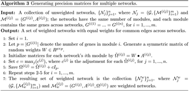
Generating precision matrices for multiple networks

If multiple networks are being constructed, it should be considered whether or not common gene-gene associations across networks should be given the same weight. By giving common edges the same weight, the only difference between networks will be the network structure itself; some edges may be missing or added within a network, but any edge present in multiple networks will have the same association strength. In order to accomplish this, the weight matrix W generated for a given module must be the same across networks, and the adjustment c used to create the precision matrix module must also be constant.

Algorithm 3 outlines the procedure for generating precision matrices for multiple networks. To reiterate, the key attribute of this algorithm is that common edges across networks will be given the same weight. If this property is not desired, then the individual networks can be weighted by iteratively running the algorithm with a single network as the input.

2.3. Generating RNA-seq data

The final step of the simulator is to generate data from the GGM and convert those values into expression data. There are two goals in creating these data: (1) The gene expression has a dependence structure that reflects the global network structure, and (2) the marginal distribution of expression for each gene resembles the reference RNA-seq data.

The generator is divided into two parts to tackle these goals. First, initial data are generated and aggregated together from the local GGMs defined in each module; this imposes the module dependence structures onto the gene expression. Then, the Gaussian values are transformed into RNA-seq data by sampling from the empirical distribution of the reference dataset. These two steps are detailed in the following sections.

Initializing values from local GGMs

Given a weighted network ${\mathcal{N}}^w=\left(\mathcal{G},{\left\{{\mathcal{M}}_w^{(i)}\right\}}_{i=1}^m\right)$, the first step is to generate a local expression vector, ${\tilde{X}}^{(j)}\in R^{\left|G^{(j)}\right|}$, for each module j = 1, …, m; the tilde here is used to distinguish these initial Gaussian values from the eventual RNA-seq data. Based on the GGM of each module, the local expression vector is generated from the multivariate normal distribution, ${\tilde{X}}^{(j)}~N\left(0,{\left({\Omega }^{(j)}\right)}^{-1}\right)$, where the mean μ = 0 is the zero vector of appropriate length. A sample can be obtained from this distribution by first generating independent standard normal variables Z_i ~ N(0, 1), setting Z^(j) = (Z₁, …, Z_p)^⊤, and transforming them by ${\tilde{X}}^{(j)}=\mu +{\Sigma }^{1/2}{Z}^{(j)}$, where ${\Sigma }^{1/2}{\left({\Sigma }^{1/2}\right)}^T={\left({\Omega }^{(j)}\right)}^{-1}$.

The global expression, $\tilde{X}\in R^{|\mathcal{G}|}$, is calculated by aggregating the expression over all modules. Consider gene $i\in \mathcal{G}$, and let M_i = {j : i ∈ G^(j)} denote the set of module indices that contain gene i. If the gene does not belong to any module (M_i ≠ ∅), then its global expression, ${\tilde{X}}_i$, is generated directly from the standard normal distribution. Otherwise, its expression is calculated by ${\tilde{X}}_i={\left|M_i\right|}^{-1/2}{\sum }_{j\in M_i}{\tilde{X}}_i^{(j)}$, where ${\tilde{X}}_i^{(j)}$ denotes the generated expression of this gene in the jth module. Rather than averaging, the weight |M_i|^−1/2 is used so that the variance of the aggregated expression remains constant; $E\left({\tilde{X}}_i\right)={\left|M_i\right|}^{-1/2}{\sum }_{j\in M_i}E\left({\tilde{X}}_i^{(j)}\right)=0$ and $Var\left({\tilde{X}}_i\right)={\left|M_i\right|}^{-1}{\sum }_{j\in M_i}Var\left({\tilde{X}}_i^{(j)}\right)=1$.

This procedure results in a random expression ${\tilde{X}}_i~N(0,1)$ for each gene such that the covariance between two genes i and j is

$$Cov\left({\tilde{X}}_i,{\tilde{X}}_j\right)=\{\begin{array}{c}\begin{array}{c}0\\ {\left|M_i\right|}^{-1/2}{\left|M_j\right|}^{-1/2}\sum _{k\in M_i\cap M_j}{\left({\Omega }^{(k)}\right)}_{ij}^{-1}\end{array}\end{array}\begin{array}{l}\text{if}{M}_i\cap M_j=\varphi \hfill \\ \text{otherwise}\hfill \end{array},$$ (5)

where ${\left({\Omega }^{(k)}\right)}_{ij}^{-1}$ is the covariance between the two genes in the kth module.

Note that, although two genes will be uncorrelated if they are in distinct modules, their partial correlation may be nonzero if the modules overlap. This means that in the presence of overlapping modules, genes with no direct connection may have nonzero partial correlation. Whether or not this property is appropriate depends on the user’s model of the data generating process. In particular, we must decide if it is appropriate to model gene expression as the aggregate of independent pathways (modules), or if expression is dependent on the global dependencies alone (collapse the modules into a single, large module). The answer to this question is not clear from a biological perspective, so SeqNet is designed to handle both cases.

The network can be coerced into a single module, which interprets all connections as global connections (this is illustrated in Section 4). In this case, the initialized expression values, ${\tilde{X}}^{(1)}$, provide the global values; no aggregation is needed since there is only one module. These generated values have all of the usual properties of a GGM. In particular, the nonzero partial correlations will correspond to direct connections (edges) in the network - this is the main distinction between generating value from a single module compare to aggregating over multiple overlapping modules.

Converting GGM values to RNA-seq data

Once the Gaussian values, ${\tilde{X}}_i~N(0,1)$ for $i\in \mathcal{G}$, are obtained, the final step is to convert these into RNA-seq data. The conversion is performed for each gene, one at a time, using the empirical marginal distribution of expression from the reference RNA-seq data.

Let $Y\in R^{n_{\text{ref}}\times \left|\mathcal{G}\right|}$ denote the reference dataset containing n_ref samples, and $F_i(x)={\sum }_{j=1}^{n_{\text{ref }}}I\left(Y_{ji}\le x\right)/n_{\text{ref }}$ denote the empirical CDF of the expression for the ith gene. Then, the conversion follows by setting $X_i=F_i^{-1}\left(\Phi \left({\tilde{X}}_i\right)\right)$, where Φ(x) is the CDF of the standard normal distribution. The inverse of the empirical CDF is calculated in R using the quantile() function with argument type set to 1, which defines the inverse CDF as $F_i^{-1}(p)=Y_i{}_{\left(\lfloor p{n}_{\text{ref}}\rfloor \right)}$, where Y_i(k) is the kth order statistic of Y_i. The procedure is summarized in Algorithm 4.

The expression values of a given gene in the reference are assumed to be identically distributed. However, raw RNA-seq counts will fail to satisfy this assumption due to differences in library sizes, GC content, batch effects, and other sources of technical and biological variation (Hitzemann, Bottomly, Darakjian, Walter, Iancu, Searles, Wilmot, and McWeeney 2013; Chowdhury et al. 2019). Therefore, it is assumed that the data have been appropriately normalized to allow for comparisons across samples using, for example, TMM normalization (Robinson and Oshlack 2010), sva (Leek and Storey 2007; Parsana et al. 2019), svapls (Chakraborty, Datta, and Datta 2012), or RUV (Freytag, Gagnon-Bartsch, Speed, and Bahlo 2015; Jacob, Gagnon-Bartsch, and Speed 2016).

3. Validation

In this section, we assess the simulator in terms of the topological properties of the generated networks and how well the generated data resemble the reference RNA-seq dataset.

3.1. Network topology

Three topological measures are commonly used to characterize networks; these include the degree distribution, clustering coefficient, and average path length. These measures have been used to describe the structure of various complex networks and to assess network generators (Barabasi and Oltvai 2004; Di Camillo et al. 2009).

Let V denote a random node sampled from the nodes in a graph, v ∈ G. The properties of a network are described on two levels: by the local characteristics with respect to V, and by the global characteristics with respect to G. In this setup, V is a random variable with P (V = v) = n⁻¹ for v ∈ G and zero otherwise, where n = |G| is the number of nodes in G. In general, local properties of a topological measure m(v) are expressed in terms of its distribution P (m(V)), while global properties are viewed by its expectation E(m(V)).

Degree

The degree of a node, d(v), is the number of connections to v. The degree of network is said to follow a power-law distribution if

$$P(d(V)=k)\propto k^{-\gamma }.$$ (6)

Networks with a power-law degree distribution are called scale-free networks (Albert and Barabási 2002). Such networks contain hub nodes that have many more connections than the average node. In biological networks, the parameter γ is often between 2 and 3 (Milo, Shen-Orr, Itzkovitz, Kashtan, Chklovskii, and Alon 2002). However, the degree distribution of transcription networks may not be so simple. For example, the exponentially truncated power law, which has the form P (d(V) = k) ∝ k^−γ exp(−αk), may be more suitable for some networks (Zhang and Horvath 2005; Csányi and Szendrői 2004). In this study, the degree distribution for various networks are compared visually rather than fitting any particular model.

The average degree of the network,

$$d(G)=E(d(V))=n^{-1}\sum _{v\in G}d(v),$$ (7)

provides a global characterization of the graph.

Clustering coefficient

The local clustering coefficient, C(v), of a node is the probability that two of its neighbors are connected. It is defined for nodes of degree d(v) ≥ 2 by,

$$C(v)=\frac{2q(v)}{d(v)(d(v)-1)}=\frac{\#\text{of}v’\text{s}\text{neighbors}\text{that}\text{are}\text{connected}}{\#\text{of}\text{possible}\text{connections}\text{among}v’\text{s}\text{neighbors}},$$ (8)

where q(v) is the number of connections among v’s neighbors. For nodes with one or fewer neighbors, C(v) is undefined.

Visually, suppose nodes j and k are connected and are neighbors of i. Then, the three nodes i–j–k form a triangle in the network. This is what the clustering coefficient measures - the frequency of triangles in the network. As a function of node degree, the average local clustering coefficient has been shown to follow a power-law distribution,

$$C(k)=E(C(V)\mid d(V)=k)\propto k^{-\varphi },$$ (9)

with ϕ = 1 for metabolic networks (Ravasz, Somera, Mongru, Oltvai, and Barabási 2002; Barabasi and Oltvai 2004); the power-law scaling of C(k) is characteristic of a hierarchical organization that is not always found in scale-free networks (Ravasz et al. 2002). As with the degree distribution, C(k) will be compared visually for various networks rather than fitting any particular model.

The global clustering coefficient provides a measure of the entire network. It is defined by,

$$C(G)=\frac{\#\text{of}\text{triangles}\text{in}G}{\#\text{of}\text{connected}\text{triples}\text{in}G}$$ (10)

Note, this is not equivalent to the average local clustering coefficient, $n^{-1}{\sum }_{v\in G}C(v)$. The global clustering coefficient is calculated using the transitivity() function from the igraph R package.

Average path length

The third measure is based on the shortest path between nodes. In particular, the average path length, L(v), for node v is,

$$L(v)=\frac{1}{|G(v)|-1}\sum _{w\in G(v)}\text{Length}\text{of}\text{shortest}\text{path}\text{between}v\text{and}w,$$ (11)

where G(v) denotes the largest connected component of G that contains v, and |G(v)| is the number of nodes in G(v). This measure is calculated using the distances() function from the igraph R package. As with the clustering coefficient, we consider the average path length as a function of node degree,

$$L(k)=E(L(V)\mid d(V)=k).$$ (12)

The global measure is the average shortest path among all pairs of nodes,

$$L(G)=n^{-1}\sum _{v\in G}L(v).$$ (13)

This measure is sometimes referred to as the characteristic path length. It is calculated using the mean_distance() function from the igraph R package.

When studying a network generating model, it can be useful to study the global characteristics as a function of network size N. For example, consider the characteristic path length as a function of network size, L(N) = E(L(G||G| = N), where G is now a random network sampled from the generating procedure. It has been shown that scale-free networks with exponent 2 < γ < 3 are ultrasmall (Cohen and Havlin 2003), having an average path length that scales by L(N) ~ log log N, compared to small-world networks whose average path length scales by log N. Similar characterizations can be made with d(N), the expected average degree, and C(N), the expected global clustering coefficient, of networks of size N. However, when comparing a network generated by SeqNet to the E. coli transcription network, comparisons of the global characteristics will be made at the fixed size N of the transcription network.

3.2. E. coli transcription network

In this section we compare the topology of a generated SeqNet network to the E. coli transcription network obtained from RegulonDB (Santos-Zavaleta et al. 2018) and to networks generated from GeneNetWeaver (Schaffter et al. 2011), SynTReN (Van den Bulcke et al. 2006), and Rogers (Rogers and Girolami 2005), obtained from the GRNdata R package (Bellot et al. 2018).

RegulonDB provides the strength of evidence for each regulatory interaction, coded as either “strong” or “weak”. When constructing the E. coli transcription network, we must choose whether to include only “strong” sources of evidence, or both “strong” and “weak” sources. There are currently 2767 connections that have strong evidence and 1797 connections with weak evidence. The network topology will change depending on whether or not the “weak” connections are included, so we consider both scenarios.

The SeqNet generator has many parameters that can be adjusted. However, in this example only ν will be adjusted, which controls the amount of overlap among modules; the remaining parameters are set to default values. As we will see, the change that occurs in the E. coli network topology when adding “weak” connections can be modeled by simply decreasing ν to allow for more connections in the generated network.

Strong evidence only

In the first case, only connections with strong evidence are included in the E. coli network. The SeqNet generator is set with v = 10⁻³ and default values for all other parameters. All five networks are shown in Figure 1. The main feature visible from this view is the presence of very large hub genes. Notably, the network generated by Rogers does not contain any large hubs.

Figure 1:

From left to right: the E. coli transcription network using only ”strong” evidence connections; a network generated from SeqNet with ν = 10⁻³; a network generated by GeneNetWeaver; a network generated by SynTReN; and a network generated by Rogers. Nodes are scaled by their degree.

The local topology for each network is summarized in Figure 2. The first column provides the degree distribution of each network. In a scale-free network, the points will follow a linear trend. But each distribution, aside from Rogers, has a longer tail than expected in a power-law distribution; this tail indicates the presence of very large hub genes. These results are consistent with previous findings that suggest biological networks deviate from a scale-free topology (Stumpf and Ingram 2005; Stumpf, Wiuf, and May 2005; Khanin and Wit 2006). However, we are not particularly interested in whether the networks are scale-free, but rather, whether the topology of the generated networks are similar to that of the E. coli transcription network.

Figure 2:

The local topologies P (k) (first column), C(k) (second column), and L(k) (third column) for A. the E. coli transcription network and generated networks from B. SeqNet, C. GeneNetWeaver, D. SynTReN, and E. Rogers. The x and y axes are shown on a log scale.

The second and third columns of Figure 2 show the clustering coefficient and average path length, respectively, as a function of node degree. These tend to follow the linear trend more closely. The power-law distribution for the clustering coefficient, C(k), has been previously identified in biological networks (Ravasz et al. 2002). However, to our knowledge the distribution of L(k) has not been previously characterized. These results from the E. coli transcription network suggests that L(k) may also follow a power-law distribution in biological networks.

Focusing on the SeqNet network (row B), the degree distribution and average path length (first and third columns) have very similar patterns compared to the E. coli network (row A). The main difference is found with the clustering coefficient, in which the E. coli network contains more variability in the clustering coefficient among genes of the same degree compared to the SeqNet network.

The global topology for each network is summarized in Table 1. The sparsity, average degree, and average path length of the SeqNet generated network are all similar to the E. coli network. The average degree for the GeneNetWeaver and SynTReN networks are much larger than the E. coli network, and similarly, their average path length is smaller. GeneNetWeaver most closely matches the E. coli network in terms of clustering coefficient.

Table 1:

Global network characteristics.

	E. coli	SeqNet	GeneNetWeaver	SynTReN	Rogers
Num. nodes	1254	1254	1477	1000	1000
Num. edges	2351	2254	3565	2319	1347
Sparsity	0.00299	0.00287	0.00327	0.00465	0.00270
Avg. degree	3.75	3.59	4.83	4.64	2.69
Clustering coef.	0.019	0.036	0.016	0.026	0.004
Avg. path length	4.24	4.70	3.58	3.70	7.68

Strong and weak connection

Next, we consider including the connections with weak evidence into the E. coli network. By including more edges, the network will become more dense. To reflect this change, the SeqNet generator is re-run with ν decreased from 10⁻³ to 10⁻² to allow for more overlap among modules which will increase density. The new E. coli and SeqNet networks are shown in Figure 3.

Figure 3:

E. coli transcription network with both ”weak” and ”strong” evidence connections (left) and a generated SeqNet network with ν = 10⁻² (right).

The topology of the E. coli network remains relatively unchanged at the local level (see Figure 4) compared to the network with only “strong” connections, but the global characteristics change (see Table 2); as we might expect after including additional connections, the average degree increases and the average path length decreases. Similar changes are found in the SeqNet network after decreasing ν from 10⁻³ to 10⁻².

Figure 4:

The local topologies of P (k), C(k), and L(k) for A. the E. coli transcription network and enerated networks from B. SeqNet. The x and y axes are shown on a log scale.

Table 2:

Global network characteristics.

	E. coli	SeqNet	GeneNetWeaver	SynTReN	Rogers
Num. nodes	1780	1780	1477	1000	1000
Num. edges	4144	3805	3565	2319	1347
Sparsity	0.00262	0.00240	0.00327	0.00465	0.00270
Avg. degree	4.66	4.28	4.83	4.64	2.69
Clustering coef.	0.015	0.035	0.016	0.026	0.004
Avg. path length	3.60	3.63	3.58	3.70	7.68

The sparsity, average degree, and average path length of the SeqNet generated network are again very similar to the E. coli network. The average degree and average path length for the GeneNetWeaver and SynTReN networks now agree with the updated values for the E. coli network. The clustering coefficient is unchanged when adding the weak connections, and the SeqNet clustering coefficient remains larger, as before.

3.3. Comparing generated data to reference data

SeqNet is able to simulated expression data that resemble a reference dataset. This is validated in two ways. First, the mean and variance of gene expression profiles are compared between the reference data and the simulated data. Second, since the main use of SeqNet is to assess the performance of co-expression methods, we compare the behavior of several such methods on the reference data compared to the simulated data. Details are provided in the following sections.

Reference RNA-seq datasets

Four RNA-seq datasets were downloaded from LinkedOmics (Vasaikar, Straub, Wang, and Zhang 2017), a portal to multi-omics data generated by The Cancer Genome Atlas (TCGA). Data were obtained for four cancers: breast invasive carcinoma, glioma, head and heck squa-mous cell carcinoma, and prostate adenocarcinoma. The downloaded datasets contain Reads Per Kilobase Million (RPKM) normalized, log₂(x + 1) transformed expression levels for transcripts annotated at the gene level. Since RPKM normalization does not align gene expression across samples (Lin, Golovnina, Chen, Lee, Negron, Sultana, Oliver, and Harbison 2016), we applied the Trimmed Mean of M-Values (TMM) normalization (Robinson and Oshlack 2010) to the untransformed RPKM data. The TMM-normalized values for each cancer were then used as four reference RNA-seq datasets (without the log transformation).

Due to computational restrictions of some co-expression methods used later, only a subset of genes in each reference dataset is used. However, since we are interested in analyzing co-expression, a random selection of genes would not be ideal because the sampled genes may be unrelated. A better strategy is to randomly sample a set of gene regulatory pathways, and subset the data onto the genes contained in those pathways. This way, the reference data will likely retain some true co-expression patterns among the sampled genes. In this study, 20 pathways are randomly sampled from the Reactome database (Fabregat, Sidiropoulos, Garapati, Gillespie, Hausmann, Haw, Jassal, Jupe, Korninger, McKay et al. 2015). Note, the main results in this section are robust to different sets of sampled pathways (results not shown).

Results for the breast cancer reference dataset are reviewed in the following sections. Similar results are obtained for the other three reference data; those details are provided in Appendix B. The breast cancer dataset contains 1093 RNA-seq samples and 15034 genes. Subsetting the data on 20 random pathways resulted in 621 unique genes.

Mean and variance of expression profiles

The first experiment verifies that the simulated expression profiles are similar to those in the reference data. A key feature of RNA-seq data is the presence of overdispersion; the gene expression profiles tend to have much larger variance compared to their mean. This motivates the use of a mean-variance plot to summarize the distribution of expression profiles. That is, the columns of each dataset will be summarized by their mean and variance, and the distribution of mean-variance pairs will be compared across datasets.

In Figure 5, a reference dataset is compared to simulated data using SeqNet and simulated data from a zero-inflated negative binomial (ZINB) model; details for the ZINB model are provided in Appendix A. A smoothed kernel density estimate is displayed to highlight the shape of each distribution. The outlying points are expression profiles with a density estimate below 0.05. We find that the overall mean-variance relationship is similar across datasets, but the outlying profiles - particularly those with excess variance - show up with the SeqNet generator but are missed by the negative binomial model.

Figure 5:

Mean-variance plots on a log scale for the reference dataset (left) and simulated data using SeqNet (middle) and a ZINB model (right). The heatmap shows a smoothed kernel density estimate. Outlying points are expression profiles with a density estimate below 0.05.

Values from co-expression methods

In the second experiment, we verify that co-expression methods produce similar association values on simulated data as they do on the reference dataset; references for these methods are provided in Section 5.1. Each co-expression method produces an association score for each gene-gene pair. For p genes, this results in p(p−1)/2 different values. In this assessment, each method is applied to the reference dataset, simulated data from the SeqNet generator, and simulated data from the zero-inflated negative binomial model; the results for each method are summarized by a histogram of the values generated from each dataset.

To simulate data, an underlying network of gene-gene associations must be provided. Since our goal is to show that the associations in simulated data can resemble those in real data, the underlying network is estimated directly from the reference dataset. This way, the associations in the simulated data are close to those in the reference. Results are shown in Figure 6. We find that for each method the values follow a similar distribution in each of the three datasets. The SeqNet and negative binomial datasets tend to generate substantial overlap and are indistinguishable for most methods. There is some difference in the simulated and reference datasets, particularly for the correlation methods and ARACNE, but these may be due to genuine differences in the true underlying network and estimated network structures.

Figure 6:

Distribution of association scores from 12 network inference methods. The underlying network is based on the estimated partial correlations in the reference dataset.

SeqNet can also be used to test the null case: what values do the co-expression methods produce when there are no gene-gene associations in the simulated data? In this case the reference dataset is not changed, but network structure is now empty; simulated data will contain independent gene expression profiles. Results from this experiment are shown in Appendix B. Most co-expression methods produce association values near zero, as expected. However, the methods CLR and Silencer continue to produce association scores that are relatively large.

4. Package usage

The main SeqNet functions are illustrated through a few working examples. A complete reference manual is available from the Comprehensive R Archive Network (CRAN); it contains additional examples, a description, and argument details for every function. The manual can be accessed in R using the help() function. SeqNet can be installed directly from CRAN and loaded using the following commands.

R> install.packages(“SeqNet”)
R> library(“SeqNet”)

A description of the main functions are provided in Table 3. The package manual contains additional details for all SeqNet functions and their arguments. This documentation is conveniently accessible within R using the help() command:

R> help(package = “SeqNet”) // To access the package manual.
R> ?random_network // Documentation for the random_network() function.

Table 3:

Summary of the main SeqNet functions.

Function	Description
random_network()	Generate a random network containing p nodes (genes). Additional tuning parameters for the network generating algorithm can be used here, including nu, prob_rewire, prob_remove, and alpha.
as_single_module()	Used to coerce a network into a single, large module rather than a collection of overlapping modules. This affects how data are generated when passed into gen_rnaseq(), as discussed in Section 2.3.1. The decision to use this function should be based on the user’s model of the data generating process.
perturb_network()	Rewires a network to obtain a differential network. By default, a hub node is randomly sampled from the network, and each of its connections are removed with probability 0.5. Note, this function can be used iteratively to turn off many hub nodes.
gen_partial_correlations()	Generates weights for the connections in a network. When multiple network objects are provided, connection that are common across networks are given the same weight.
print()	Printing a network displays the number of nodes, edges, and modules, along with the average degree, clustering coefficient, and average path length in the network.
plot()	Generates a plot of the network. See also plot_network().
plot_network_diff()	Generates a plot of the differential network between two network objects.
gen_rnaseq()	Generate an RNA-seq dataset containing n samples (rows) with a dependence structure defined by a given network. A reference dataset can be provided.
sample_reference_data()	Helper function for sampling p genes (columns) from a reference dataset. The argument percent_ZI is useful when the reference contains zero-inflated genes to control the proportion of the p sampled genes that are zero-inflated.
get_adj acency_matrix()	Creates an adjacency matrix from a network. If genes i and j are connected in the network (in any module), then the ijth entry of the adjacency matrix is 1, and otherwise is 0.
create_network_from_adj acency_matrix()	Creates a network from an adjacency matrix. This is useful when the user has a prespecified network structure, i.e. doesn’t want to generate a random one, but does want to generate RNA-seq data.

The two main SeqNet functions are random_network() and gen_rnaseq(). These can be used to quickly generate a random network of p genes and simulate an RNA-seq dataset of n samples.

R> p <- 100 # Number of nodes (genes) in the network.
R> n <- 100 # Number of samples to generate.
R> network <- random_network(p) # Create a random network of size p.
R> generated_data <- gen_rnaseq(n, network) # Generate n samples.

The variable generated_data is a list containing the generated dataset (containing n rows and p columns) and the reference dataset used to create them. Note that the network is not weighted; when gen_rnaseq() is called, it automatically uses gen_partial_correlations() to generate weights for the network. Additionally, no reference dataset is provided to gen_rnaseq(); in this case, gen_rnaseq() uses the breast cancer dataset by default.

The above code is a minimal example to quickly generate RNA-seq data. However, better practice is to explicitly code the intermediate steps.

R> p <- 100 # Number of nodes (genes) in the network.
R> n <- 100 # Number of samples to generate.
R> network <- random_network(p) # Create a random network of size p.
R> network <- gen_partial_correlations(network) # Generate weights.
R> df_ref <- SeqNet::reference$rnaseq # The reference dataset.
R> generated_data <- gen_rnaseq(n, network, df_ref) # Generate n samples.

This code shows how the user can generate weights for the network object and access the breast cancer reference data. Note that SeqNet::reference$rnaseq can be replaced by the user’s preferred reference data. In addition, any normalization or transformations can be applied to these data before passing it into gen_rnaseq().

The next example illustrates simulating two populations. This is useful, for example, to generate data for a differential network analysis. In most applications, the two networks should be similar overall with only a few connections changed. To achieve this, the perturb_network() function is used to introduce differential connections (perturbations) to the first network. In addition, this example will demonstrate how to coerce a network to a single module using the as_single_module() function (refer to Section 2.3.1 for details). The networks are visualized using plot(), and the layout of each display can be passed from one plot to the other for easier comparison, as will be shown.

R> set.seed(1) # Set the random number generator seed for reproducibility.
R> network_1 <- random_network(p) # Create a random network of size p.
R> network_2 <- as_single_module(network_1)
R> g <- plot(network_1) # Save the plot as variable g.

# Create the second network by rewiring 2 hub genes and 10 non-hub genes.
R> network_2 <- perturb_network(network_1, n_hubs = 2, n_nodes = 10)
R> plot(network_2, g) # Plot network_2 using same node layout as network_1.

At this stage, we have generated two random networks, network_1 and network_2. Both of these networks have been plotted, but it is difficult to compare the two images. For easier comparison, the plot_network_diff() function is used to plot the differential network. Here, tan edges are connections only present in the first network, red edges are only present in the second network, and black edges are common to both networks. In addition, the size of each node is proportional to the number of differential connections (tan or red edges), which helps identify differentially connected nodes. Note that saving the original plot, g, allows us to maintain the same layout across different plots.

# Can also compare two networks by a differential network visualization: R> plot_network_diff(network_1, network_2, g) # Use g to maintain the layout.

To generate precision matricies for these two networks, the gen_partial_correlations() function is used. When passing more than one network into this function, it returns a list of weighted networks.

R> network_list <- gen_partial_correlations(network_1, network_2)
R> network_1 <- network_list[[1]] # Take the weighted networks from the list.
R> network_2 <- network_list[[2]]

These weighted networks can then be used to generate RNA-seq data. The breast cancer dataset is used, and it is subset onto p genes prior to passing it into the generator using the sample_reference_data() function. Using the same p reference genes for both generated datasets ensures that the marginal distribution of each gene is the same in both networks and only the conditional dependences among the genes change. Alternatively, different references can be used for the two populations, which would allow us to simulate differential expression in addition to differential connectivity.

R> df_ref <- SeqNet::reference$rnaseq # The breast cancer reference dataset.
R> df_ref <- sample_reference_data(df_ref, p) # Subset onto p genes.
R> x_1 <- gen_rnaseq(n, network_1, df_ref)$x # Generated data for network 1.
R> x_2 <- gen_rnaseq(n, network_2, df_ref)$x # Generated data for network 2.

The generated datasets x_1 and x_2 can be used, for example, to assess the performance of a differential network analysis procedure. In that case, the estimated differential network will be compared to the true differential network, which can be obtained as an adjacency matrix using the get_adjacency_matrix() function:

R> adj_1 <- get_adjacency_matrix(network_1)
R> adj_2 <- get_adjacency_matrix(network_2)
# The differential network represented as an adjacency matrix:
R> adj_diff <- abs(adj_1 - adj_2)
R> plot_network(adj_diff, g) # Use g to maintain same layout.

Here, adj_diff is the adjacency matrix for the differential network, and it can be visualized just like a network object using the plot_network() function. Any adjacnecy matrix can also be used to create a network object with the create_network_from_adjacency_matrix() function:

R> network <- create_network_from_adjacency_matrix(adj_1)

This can be useful if the user wants to manually modify the structure generated by random_network() or to use a pre-specified network structure to generate RNA-seq data from. Note, however, that the adjacency matrix only specifies the global connections (it does not contain information on modules), so the created network will consist of a single module containing all of those global connections. (This is similar to applying the as_single_module() function to a network object.)

5. Application

The SeqNet package provides a set of tools for creating gene-gene networks and simulating gene expression data from them. These tools can be used in many applications: for example, (1) to compare the performance of various co-expression methods in a particular setting; (2) to explore how robust a method is to assumptions on network topology or distribution of gene expression; (3) to determining whether different transformations of the data improve performance; (4) to display the estimated network and visually compare it to the true underlying network; (5) to determine if a method is able to identify certain motifs in the underlying network; and (6) to assess the performance of differential network analysis methods (Gill, Datta, and Datta 2010; Fukushima 2013; Ha et al. 2015; Ji, He, Feng, He, Xue, and Xie 2017; Siska and Kechris 2017; Grimes, Potter, and Datta 2019).

The range of applications is too broad to fully cover in this manuscript. Instead, a single application is selected and covered in detail. In this application, SeqNet will be used to assess the performance of 12 co-expression networks in various settings; these settings include three different topologies for the underlying network and three different marginal distributions for the expression data. The goal is to determine how these settings affect the relative performance of each method. This application illustrates the two main utilities of SeqNet: the ability to implement any network structure, and to generate expression data under various distributions.

The R code for this application involves the use of external packages (methods for estimating networks and assessing performance). Since the bulk of code is not specific to the SeqNet package, those details are left as Supplements in the replication materials.

5.1. Co-expression methods

Twelve co-expression methods are considered: ARACNE (Margolin, Nemenman, Basso, Wiggins, Stolovitzky, Dalla Favera, and Califano 2006), BC3NET (Matos Simoes and Emmert-Streib 2012), C3NET (Altay and Emmert-Streib 2010), CLR (Faith et al. 2007), DWLasso (Sulaimanov, Kumar, Burdet, Ibberson, Pagni, and Koeppl 2018), GENIE3 (Huynh-Thu, Irrthum, Wehenkel, and Geurts 2010), glasso (Friedman, Hastie, and Tibshirani 2008), MR-NET (Meyer, Kontos, Lafitte, and Bontempi 2007), Pearson correlation, Shrinkage (Schäfer and Strimmer 2005), Silencer (Barzel and Barabási 2013), and Spearman correlation. Each of these methods take in steady-state expression data and produce gene-gene association values to create an undirected network.

The minet R package (Meyer, Lafitte, and Bontempi 2008) is used to run ARACNE, CLR, and MRNET; the default settings for these three methods were used, which includes using “spearman” as the entropy estimator. The bc3net R package (Matos Simoes and Emmert-Streib 2012) provides an implementation of BC3NET and C3NET; the default settings were used, except the entropy estimator was changed from “pearson” to “spearman” so that all MI-based methods use the same estimator. The degree weighted lasso, DWLasso, is implemented in the DWLasso R package (Sulaimanov et al. 2018). GENIE3, which is a regression tree based method, is implemented in the GENIE3 R package (Huynh-Thu et al. 2010); the default number of trees was decreased from 1000 to 100 due to computational restrictions. The graphical lasso, glasso, is implemented using the glasso R package (Friedman, Hastie, and Tibshirani 2018); the regularization parameter was set to 0.1 for all simulations. The shrinkage approach to covariance estimation, Shrinkage, is implemented in the corpcor R package (Schafer, Opgen-Rhein, Zuber, Ahdesmaki, Silva, and Strimmer. 2017). The silencing of indirect correlations method, Silencer, was translated from existing MATLAB code (Barzel and Barabási 2013) into R code. The Pearson and Spearman correlations were both implemented using the base R function cor().

5.2. Performance measures

Inferring the connections in a gene-gene network can be viewed as a binary classification problem, in which every gene-gene pair is classified as connected or not connected. The co-expression methods produce values that correspond to the estimated strengths of each gene-gene association. A network can be constructed from these values by setting a threshold and connecting any gene-gene pair with an association strength above the threshold. With a fixed threshold, the number of true positives (TP), false positives (FP), true negatives (TN), and false negatives (FN) can be calculated, and performance is evaluated using metrics such as sensitivity (also called recall), specificity, and true discovery rate (TDR; also called precision), which are defined by,

$$\text{sensitivity}=\text{recall}=\text{TP}/\left(\text{TP}+\text{FN}\right),$$

$$\text{specificity}=\text{TN}/\left(\text{TN}+\text{FP}\right),$$

$$\text{TDR}=\text{precision}=\text{TP}/\left(\text{TP}+\text{FP}\right).$$

However, this leaves the task of choosing an appropriate threshold for each method. In practice, the best threshold will likely depend on the specific problem at hand, as raising or lowering the threshold will adjust the trade-off between sensitivity and specificity. For some problems, a higher threshold may be preferred in order to increase sensitivity at the potential cost of precision, while in other settings having higher precision may be favorable.

To avoid the problem of choosing a threshold, the receiver operating characteristic (ROC) and precision-recall (PR) curves can be used. This approach considers all possible thresholds to explore the overall performance. The ROC curve plots 1 − specificty on the x-axis and sensitivity on the y-axis, and the PR curve plots recall on the x-axis and precision on the y-axis. In the context of classifying connections in the network, there is a large imbalance between the two classes; since the networks are sparse, the number of true connections will be much smaller than the number of possible connections. Because of this, using the ROC alone can provide misleading results. The PR curve avoids these problems because it does not incorporate TN, the number of true negatives, which is the term that will be inflated from the sparsity of the network and can skew the results. In the DREAM3 challenge, both ROC and PR were used to gain a full characterization of performance (Prill et al. 2010). Here, we present results for PR and provide those for ROC in Appendix C.

If a method produces a PR (or ROC) curve that dominates all other curves, then that method provides the best performance (Davis and Goadrich 2006). More often, however, the curves for each method will intersect, making the selection of a best performer more ambiguous (Bekkar, Djemaa, and Alitouche 2013). The area under the PR curve (AUC-PR) and area under the ROC curve (AUC-ROC) provide convenient summary metrics for the overall performance. Selecting the method with the highest AUC-PR makes the process less ambiguous, even if no single method produces a dominating curve. However, the method with highest AUC-PR will not necessarily be the same method with the highest AUC-ROC (Davis and Goadrich 2006).

5.3. Network structures

The SeqNet package provides a novel method for creating random networks. However, the user is not limited to the built-in network generator; any network can be used to generate gene expression data with SeqNet. In this application, three different network generating algorithms are considered: the Watts-Strogatz algorithm for generating random small-world networks (Watts and Strogatz 1998); the Barabasi-Albert method for generating scale-free networks (Barabási and Albert 1999); and the SeqNet algorithm. Figure 7 provides a visualization of networks generated by these three procedures. The performances of each co-expression method are compared across these three underlying network topologies.

Figure 7:

Example networks generated from the Watts-Strogatz algorithm (left), the Barabasi-Albert method (middle) and the SeqNet generator (right). Each network contains p = 400 genes.

5.4. Distribution of gene expression

The SeqNet package is designed to incorporate a reference RNA-seq dataset and generate expression profiles that have similar marginal distributions as the reference. In addition, the package can be used to generate data from a Gaussian graphical model, which produces normally distributed expression profiles, or it can generate data from a zero-inflated negative binomial model, which produces expression profiles having a discrete distribution resembling raw RNA-seq counts. In this application, each of these three approaches are considered. The co-expression method are compared across the three distributions. For simulating RNA-seq data, the reference used is the breast cancer dataset reviewed in Section 3.

5.5. Results

All results are from networks containing p = 400 genes and n = 200 samples. This resembles the typical setting where n < p, and the network is moderately large. The main restriction to p and n in this application were the computational limitations of some methods considered - DWLasso and GENIE3 in particular. Due to this restriction, additional values for p and n were not considered for further simulations; nevertheless, such considerations would deviate from the main purpose of this application.

The AUC-PR of each method for different network topologies are shown in Figure 8. This figure is meant to summarize each method individually, not to make comparisons across different methods. Most methods have their best performance on the Watts-Strogatz small-world network (WS), with a decrease in performance on the Barabasi-Albert scale-free networks (BA), and a further decrease on the SeqNet networks. Some exceptions are DWLasso, which attains its best performance on SeqNet networks - this makes sense because SeqNet networks contain very large hub genes, and DWLasso is designed to handle hubs; MRNET, which has similar performance on both BA and SeqNet network; and both Pearson and Spearman correlations maintain similar AUC-PR across all three topologies.

Figure 8:

AUC-PR values from 30 simulations using networks generated by the Watts-Strogatz algorithm, the Barabasi-Albert method, and the SeqNet network generator. RNA-seq expression profiles were generated with SeqNet using the breast cancer reference dataset. In general, the performance of each method depends on the underlying network topology.

The AUC-PR of each method for different marginal distributions of gene expression are shown in Figure 9. As before, this figure is meant to summarize performance within each method, not across methods. These results show that for each method the performance is similar across the three distributions. This suggests that each method is robust to the distribution of expression profiles.

Figure 9:

AUC-PR values from 30 simulations using Gaussian, RNA-seq, and negative-binomial data. The underlying network is generated using the SeqNet generator. The NB and RNA-seq data are log(x + 1) transformed. Each method has similar performance across different data types.

In Figure 10, the relative performances of each method are compared based on AUC-PR, with underlying networks generated by the Watts-Strogatz algorithm, the Barabasi-Albert method, and the SeqNet generator. In each setting, RNA-seq expression data are generated with SeqNet using the breast cancer reference dataset, and a log(x + 1) transformation is applied.

Figure 10:

AUC-PR values from 30 simulations with the underlying network generated using the Watts-Strogatz algorithm, the Barabasi-Albert method, and the SeqNet generator. The RNA-seq expression data are generated by SeqNet using the breast cancer dataset.

These results suggest that the relative performance of each method depends on the underlying network topology. For example, on WS networks the five methods ARACNE, BC3Net, CLR, glasso, and Silencer all have the best performance. But on BA networks, the two networks ARACNE and BC3Net come out on top. When considering SeqNet networks, DWLasso has a slight edge in performance, followed closely by ARACNE, BC3Net, C3Net, and MRNET.

This application demonstrates the importance of the underlying topology when assessing the relative performance of network estimation methods. With SeqNet, a wide range of topologies can be generated by varying its tuning parameters. The default settings were used in this demonstration, but a range of values should be considered in practice. For example, increasing nu lowers the average path length and increases the average degree of generated networks, while increasing alpha lowers the clustering coefficient and has minimal effect on average degree and path length. The utility of SeqNet comes from exploring these tuning parameters and evaluating the network estimation methods across a wide range of topologies.

6. Discussion

The SeqNet package provides convenient tools for assessing the performance of co-expression methods. The main feature of SeqNet is its ability to simulate RNA-seq expression data from an underlying network of gene-gene associations, and we have demonstrated that the marginal distribution of simulated data resemble those of a reference dataset. While any network can be used with SeqNet, the package also provides a novel network generator that creates random networks having a topology similar to real biological networks. The SeqNet network generator can be adjusted through various tuning parameters to access a rich distribution of network topologies – the exact relationship between these parameters and the generated topologies will be studied in a future project.

The SeqNet package is implemented in R and freely available through CRAN. The implementation uses C++ code for efficient computation. The algorithm for generating random networks runs in linear time, O(p), where p is the number of nodes in the network. On a 2.2 Ghz Intel Core i7 laptop computer, it takes an average 0.06s, 0.58s, and 7.4s to generate networks containing 10², 10³, and 10⁴ nodes, respectively. The algorithm for simulating expression data also runs in linear time, O(n), where n is the number of samples generated. On the same machine, it takes an average 0.73s, 5.5s, and 45s to simulated 10², 10³, and 10⁴ samples from a network containing 1000 nodes.

SeqNet is most useful for evaluating the performance of unsupervised co-expression methods that do not implement biological knowledge. It can be used to gain insight into how performance may change depending on the topology of the underlying network, or depending on the distribution of gene expression. SeqNet can use a reference RNA-seq dataset to simulate realistic data, however only information on the marginal distributions of read counts in the reference are used. Any additional information about the genes or samples are not taken into account. Because of this, SeqNet may have limited utility in evaluating co-expression methods that take advantage of existing domain knowledge, such as the known identity of transcription factors.

A limitation of SeqNet is its reliance on the Gaussian graphical model (GGM). This model allows us to generate data that have a particular conditional dependence structure, but the gene-gene interactions are restricted to monotonic relationships. It is uncertain how well this model is able to capture the true data generating process of gene expression. The dynamics of gene regulation are often modeled using Michaelis-Menten and Hill kinetics, but it is unclear how to simulate high-dimensional RNA-seq data from this model. Using a GGM provides a tractable approach, and our validation study suggests that it does produce data that are similar to the real datasets.

A. Zero-inflated negative binomial (ZINB) model

When the reference data contain read counts, then a zero-inflated negative binomial (ZINB) distribution can be used to model the marginal distribution of each individual gene’s expression. The probability mass function for the ZINB is defined by the mixture,

$$P_{\text{ZINB}}(X=x)=\rho I(x=0)+(1-\rho )P_{\text{NB}}(x),$$ (14)

where ρ ∈ [0, 1] and P_NB is the negative binomial (NB) distribution,

$$P_{NB}(X=x)=\frac{\Gamma (x+s)}{x!\Gamma (s)}{\left(\frac{s}{m+s}\right)}^s{\left(\frac{m}{m+s}\right)}^x$$ (15)

parameterized by its mean m > 0 and shape s > 0. The NB is a generalization of the Poisson distribution and is often used to analyze RNA-seq data (Robinson, McCarthy, and Smyth 2010; Love, Huber, and Anders 2014; Wu, Wang, and Wu 2012). The NB can model the overdispersion that is characteristic of RNA-seq data; that is, the variance of RNA-seq counts is often much larger than the mean. Overdispersion can be caused by technical variation in measuring gene expression as well as biological variation among and within samples. The ZINB extends the NB model through the zero inflation component; this term can account for instances where heterogeneity in the population results in a gene being unexpressed in a portion of the population.

The reference RNA-seq dataset is used to determine appropriate parameters θ = (m, s, ρ) for the ZINB model. For each gene, i, in the network, a random gene from the reference dataset is chosen, and the maximum likelihood estimate ${\widehat{\theta }}_i$ is calculated from that gene’s expression data.

The Gaussian data generated from the network structure are transformed into count data using the inverse transformation method. Let F (x|θ) = P_ZINB(X ≤ x|θ) denote the CDF for the ZINB distribution with parameters θ, Φ denote the CDF of the standard normal distribution, and ${\tilde{X}}_i$ denote the generated Gaussian expression for gene i. The RNA-seq counts are then obtained by,

$$X_i=F^{-1}\left(\Phi \left({\tilde{X}}_i\right)\mid {\widehat{\theta }}_i\right),$$ (16)

where y = F ⁻¹(x) satisfies P_ZINB(X < y) ≤ x ≤ P_ZINB(X ≤ y).

B. Additional results for validating generated profiles

In this section, results for the breast cancer, prostate cancer, head and neck cancer, and glioma reference RNA-seq datasets are provided. The same mean-variance plots and distribution of association scores that were utilized in Section 3.3 are used here.

B.1. Breast cancer

The breast cancer dataset contains 1093 RNA-seq samples and 15034 genes. Subsetting the data on 20 random pathways resulted in 621 unique genes. The mean-variance plots and distribution of association scores are provided in the manuscript. The association scores for the null case are shown here.

Figure A1:

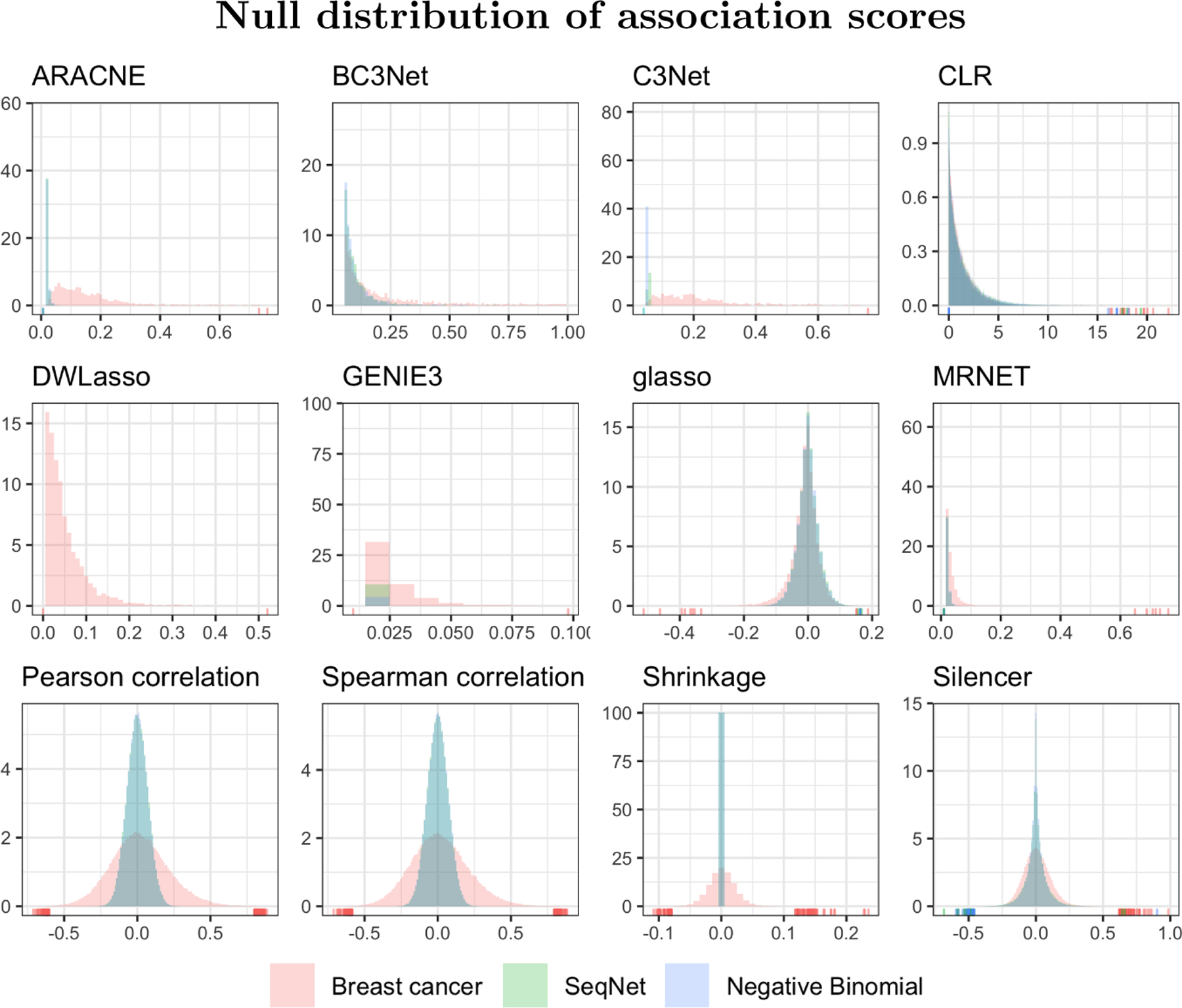
Distribution of association scores from 12 network inference methods. The SeqNet and Negative Binomial data contain independent gene expression profiles, i.e., the underlying network contains no connections.

B.2. Prostate cancer

The prostate cancer dataset contains 497 samples. Subsetting the data on 20 random Reactome pathways results in 673 unique genes.

Figure A2:

Mean-variance plots for the breast cancer reference dataset and simulated data using SeqNet and a zero-inflated negative binomial model. The blue heatmap shows a smoothed kernel density estimate, and the outlying points are expression profiles with a density estimate below 0.05. The axes are drawn on a log scale.

Figure A3:

Distribution of association scores from various network inference methods. The underlying network used by SeqNet is based on the estimated partial correlations in the reference dataset.

Figure A4:

Distribution of association scores from various network inference methods. The SeqNet and Negative Binomial data contain independent gene expression profiles, i.e. the underlying network contains no connections.

B.3. Head and neck cancer

The head and neck cancer dataset contains 520 samples. Subsetting the data on 20 random Reactome pathways results in 726 unique genes.

Figure A5:

Mean-variance plots for the breast cancer reference dataset and simulated data using SeqNet and a zero-inflated negative binomial model. The blue heatmap shows a smoothed kernel density estimate, and the outlying points are expression profiles with a density estimate below 0.05. The axes are drawn on a log scale.

Figure A6:

Distribution of association scores from various network inference methods. The underlying network used by SeqNet is based on the estimated partial correlations in the reference dataset.

Figure A7:

Distribution of association scores from various network inference methods. The SeqNet and Negative Binomial data contain independent gene expression profiles, i.e. the underlying network contains no connections.

B.4. Glioma

The Glioma dataset contains 667 samples. Subsetting the data on 20 random Reactome pathways results in 538 unique genes.

Figure A8:

Mean-variance plots for the breast cancer reference dataset and simulated data using SeqNet and a zero-inflated negative binomial model. The blue heatmap shows a smoothed kernel density estimate, and the outlying points are expression profiles with a density estimate below 0.05. The axes are drawn on a log scale.

Figure A9:

Distribution of association scores from various network inference methods. The underlying network used by SeqNet is based on the estimated partial correlations in the reference dataset.

Figure A10:

Distribution of association scores from various network inference methods. The SeqNet and Negative Binomial data contain independent gene expression profiles, i.e. the underlying network contains no connections.

C. Additional results from the application

This section provides results for the AUC-ROC metric, along with full PR and ROC curves. The same general conclusions made in the manuscript for AUC-PR can be made for AUC-ROC; the performance of each method depends on the topology of the underlying network but is robust to different distributions of gene expression. However, there is less variability in AUC-ROC when comparing methods on a fixed network topology; each method provides similar performance in terms of AUC-ROC. This is in contrast to AUC-PR, which produced more separation in performance among the methods.

Figure A11:

AUC-ROC values from 30 simulations using networks generated by the Watts-Strogatz algorithm, the Barabasi-Albert method, and the SeqNet network generator. RNA-seq expression profiles were generated with SeqNet using the breast cancer reference dataset. In general, the performance of each method depends on the underlying network topology.

Figure A12:

AUC-ROC values from 30 simulations using Gaussian, RNA-seq, and negative-binomial data. The underlying network is generated using the SeqNet generator. The NB and RNA-seq data are log(x + 1) transformed. Each method has similar performance across different data types.

Figure A13:

AUC-ROC values from 30 simulations with the underlying network generated using the Watts-Strogatz algorithm, the Barabasi-Albert method, and the SeqNet generator. The RNA-seq expression data are generated by SeqNet using the breast cancer dataset The full PR and ROC curves are shown in the following figures. The results are separated based on the underlying network topology.

Figure A14:

PR and ROC curves from 30 simulations with the underlying network generated using the Watts-Strogatz algorithm. The RNA-seq expression data are generated by SeqNet using the breast cancer dataset

Figure A15:

PR and ROC curves from 30 simulations with the underlying network generated using the Barabasi-Albert method. The RNA-seq expression data are generated by SeqNet using the breast cancer dataset

Figure A16:

PR and ROC curves from 30 simulations with the underlying network generated using the SeqNet generator. The RNA-seq expression data are generated by SeqNet using the breast cancer dataset

References

- Albert R, Barabási AL (2002). “Statistical Mechanics of Complex Networks.” Reviews of Modern Physics, 74(1), 47. [Google Scholar]
- Altay G, Emmert-Streib F (2010). “Inferring the Conservative Causal Core of Gene Regulatory Networks.” BMC Systems Biology, 4(1), 132. [DOI] [PMC free article] [PubMed] [Google Scholar]
- Angly FE, Willner D, Rohwer F, Hugenholtz P, Tyson GW (2012). “Grinder: A Versatile Amplicon and Shotgun Sequence Simulator.” Nucleic Acids Research, 40(12), e94–e94. [DOI] [PMC free article] [PubMed] [Google Scholar]
- Barabási AL, Albert R (1999). “Emergence of Scaling in Random Networks.” Science, 286(5439), 509–512. [DOI] [PubMed] [Google Scholar]
- Barabasi AL, Oltvai ZN (2004). “Network Biology: Understanding the Cell’s Functional Organization.” Nature Reviews Genetics, 5(2), 101. [DOI] [PubMed] [Google Scholar]
- Barbosa S, Niebel B, Wolf S, Mauch K, Takors R (2018). “A Guide to Gene Regulatory Network Inference for Obtaining Predictive Solutions: Underlying Assumptions and Fundamental Biological and Data Constraints.” Biosystems. [DOI] [PubMed] [Google Scholar]
- Barrett T, Troup DB, Wilhite SE, Ledoux P, Evangelista C, Kim IF, Tomashevsky M, Marshall KA, Phillippy KH, Sherman PM, et al. (2010). “NCBI GEO: Archive for Functional Genomics Data Sets—10 Years On.” Nucleic Acids Research, 39(suppl 1), D1005–D1010. [DOI] [PMC free article] [PubMed] [Google Scholar]
- Barzel B, Barabási AL (2013). “Network Link Prediction by Global Silencing of Indirect Correlations.” Nature Biotechnology, 31(8), 720. [DOI] [PMC free article] [PubMed] [Google Scholar]
- Bekkar M, Djemaa HK, Alitouche TA (2013). “Evaluation Measures for Models Assessment over Imbalanced Data Sets.” Journal of Information Engineering and Applications, 3(10). [Google Scholar]
- Bellot P, Olsen C, Meyer PE (2018). grndata: Synthetic Expression Data for Gene Regulatory Network Inference. R package version 1.14.0.
- Benidt S, Nettleton D (2015). “SimSeq: A Nonparametric Approach to Simulation of RNA-Sequence Datasets.” Bioinformatics, 31(13), 2131–2140. [DOI] [PMC free article] [PubMed] [Google Scholar]
- Casella G, Berger RL (2002). Statistical Inference, volume 2. Duxbury Pacific Grove, CA. [Google Scholar]
- Chakraborty S, Datta S, Datta S (2012). “Surrogate Variable Analysis using Partial Least Squares (SVA-PLS) in Gene Expression Studies.” Bioinformatics, 28(6), 799–806. [DOI] [PubMed] [Google Scholar]
- Chowdhury HA, Bhattacharyya DK, Kalita JK (2019). “(Differential) Co-Expression Analysis of Gene Expression: A Survey of Best Practices.” IEEE/ACM Transactions on Computational Biology and Bioinformatics. [DOI] [PubMed] [Google Scholar]
- Cohen R, Havlin S (2003). “Scale-Free Networks are Ultrasmall.” Physical Review Letters, 90(5), 058701. [DOI] [PubMed] [Google Scholar]
- Csányi G, Szendrői B (2004). “Structure of a Large Social Network.” Physical Review E, 69(3), 036131. [DOI] [PubMed] [Google Scholar]
- Danaher P, Wang P, Witten DM (2014). “The Joint Graphical Lasso for Inverse Covariance Estimation Across Multiple Classes.” Journal of the Royal Statistical Society B, 76(2), 373–397. [DOI] [PMC free article] [PubMed] [Google Scholar]
- Davis J, Goadrich M (2006). “The Relationship Between Precision-Recall and ROC Curves.” In Proceedings of the 23rd International Conference on Machine learning, pp. 233–240. ACM. [Google Scholar]
- de Jong H (2002). “Modeling and Simulation of Genetic Regulatory Systems: A Literature Review.” Journal of Computational Biology, 9(1), 67–103. [DOI] [PubMed] [Google Scholar]
- Delagado FM, Gómez-Vela F (2019). “Computational Methods for Gene Regulatory Networks Reconstruction and Analysis: A Review.” Artificial Intelligence in Medicine, 95, 133–145. [DOI] [PubMed] [Google Scholar]
- Di Camillo B, Toffolo G, Cobelli C (2009). “A Gene Network Simulator to Assess Reverse Engineering Algorithms.” The Annals of the New York Academy of Sciences, 1158(1), 125–142. [DOI] [PubMed] [Google Scholar]
- Dobrin R, Beg QK, Barabási AL, Oltvai ZN (2004). “Aggregation of Topological Motifs in the Escherichia Coli Transcriptional Regulatory Network.” BMC Bioinformatics, 5(1), 10. [DOI] [PMC free article] [PubMed] [Google Scholar]
- Dong X, Yambartsev A, Ramsey SA, Thomas LD, Shulzhenko N, Morgun A (2015). “Reverse enGENEering of Regulatory Networks from Big Data: A Roadmap for Biologists.” Bioinformatics and Biology Insights, 9, BBI–S12467. [DOI] [PMC free article] [PubMed] [Google Scholar]
- Emmert-Streib F, Dehmer M (2018). “Inference of Genome-Scale Gene Regulatory Networks: Are There Differences in Biological and Clinical Validations?” Machine Learning and Knowledge Extraction, 1(1), 138–148. [Google Scholar]
- Emmert-Streib F, Dehmer M, Haibe-Kains B (2014). “Gene Regulatory Networks and Their Applications: Understanding Biological and Medical Problems in Terms of Networks.” Frontiers in Cell and Developmental Biology, 2, 38. [DOI] [PMC free article] [PubMed] [Google Scholar]
- Fabregat A, Sidiropoulos K, Garapati P, Gillespie M, Hausmann K, Haw R, Jassal B, Jupe S, Korninger F, McKay S, et al. (2015). “The Reactome Pathway Knowledgebase.” Nucleic Acids Research, 44(D1), D481–D487. [DOI] [PMC free article] [PubMed] [Google Scholar]
- Faith JJ, Hayete B, Thaden JT, Mogno I, Wierzbowski J, Cottarel G, Kasif S, Collins JJ, Gardner TS (2007). “Large-Scale Mapping and Validation of Escherichia Coli Transcriptional Regulation from a Compendium of Expression Profiles.” PLoS Biology, 5(1), e8. [DOI] [PMC free article] [PubMed] [Google Scholar]
- Featherstone DE, Broadie K (2002). “Wrestling with Pleiotropy: Genomic and Topological Analysis of the Yeast Gene Expression Network.” Bioessays, 24(3), 267–274. [DOI] [PubMed] [Google Scholar]
- Frazee AC, Jaffe AE, Langmead B, Leek JT (2015). “Polyester: Simulating RNA-Seq Datasets with Differential Transcript Expression.” Bioinformatics, 31(17), 2778–2784. [DOI] [PMC free article] [PubMed] [Google Scholar]
- Freytag S, Gagnon-Bartsch J, Speed TP, Bahlo M (2015). “Systematic Noise Degrades Gene Co-Expression Signals but can be Corrected.” BMC Bioinformatics, 16(1), 309. [DOI] [PMC free article] [PubMed] [Google Scholar]
- Friedman J, Hastie T, Tibshirani R (2008). “Sparse Inverse Covariance Estimation with the Graphical Lasso.” Biostatistics, 9(3), 432–441. [DOI] [PMC free article] [PubMed] [Google Scholar]
- Friedman J, Hastie T, Tibshirani R (2018). glasso: Graphical Lasso: Estimation of Gaussian Graphical Models. R package version 1.10.
- Fukushima A (2013). “DiffCorr: An R Package to Analyze and Visualize Differential Correlations in Biological Networks.” Gene, 518(1), 209–214. [DOI] [PubMed] [Google Scholar]
- Gentle JE (2007). Matrix Algebra, volume 10 of Springer Texts in Statistics. Springer-Verlag, New York, NY. [Google Scholar]
- Gill R, Datta S, Datta S (2010). “A Statistical Framework for Differential Network Analysis from Microarray Data.” BMC Bioinformatics, 11(1), 95. [DOI] [PMC free article] [PubMed] [Google Scholar]
- Griebel T, Zacher B, Ribeca P, Raineri E, Lacroix V, Guigó R, Sammeth M (2012). “Modelling and Simulating Generic RNA-Seq Experiments with the Flux Simulator.” Nucleic Acids Research, 40(20), 10073–10083. [DOI] [PMC free article] [PubMed] [Google Scholar]
- Grimes T, Potter SS, Datta S (2019). “Integrating Gene Regulatory Pathways into Differential Network Analysis of Gene Expression Data.” Scientific reports, 9(1), 5479. [DOI] [PMC free article] [PubMed] [Google Scholar]
- Ha MJ, Baladandayuthapani V, Do KA (2015). “DINGO: Differential Network Analysis in Genomics.” Bioinformatics, 31(21), 3413–3420. [DOI] [PMC free article] [PubMed] [Google Scholar]
- Hache H, Wierling C, Lehrach H, Herwig R (2009). “GeNGe: Systematic Generation of Gene Regulatory Networks.” Bioinformatics, 25(9), 1205–1207. [DOI] [PMC free article] [PubMed] [Google Scholar]
- He F, Balling R, Zeng AP (2009). “Reverse Engineering and Verification of Gene Networks: Principles, Assumptions, and Limitations of Present Methods and Future Perspectives.” Journal of Biotechnology, 144(3), 190–203. [DOI] [PubMed] [Google Scholar]
- Hitzemann R, Bottomly D, Darakjian P, Walter N, Iancu O, Searles R, Wilmot B, McWeeney S (2013). “Genes, Behavior and Next-Generation RNA Sequencing.” Genes, Brain and Behavior, 12(1), 1–12. [DOI] [PMC free article] [PubMed] [Google Scholar]
- Huynh-Thu VA, Irrthum A, Wehenkel L, Geurts P (2010). “Inferring Regulatory Networks from Expression Data using Tree-Based Methods.” PloS ONE, 5(9), e12776. [DOI] [PMC free article] [PubMed] [Google Scholar]
- Jacob L, Gagnon-Bartsch JA, Speed TP (2016). “Correcting Gene Expression Data when Neither the Unwanted Variation nor the Factor of Interest are Observed.” Biostatistics, 17(1), 16–28. [DOI] [PMC free article] [PubMed] [Google Scholar]
- Ji J, He D, Feng Y, He Y, Xue F, Xie L (2017). “JDINAC: Joint Density-Based Non-Parametric Differential Interaction Network Analysis and Classification using High-Dimensional Sparse Omics Data.” Bioinformatics, 33(19), 3080–3087. [DOI] [PMC free article] [PubMed] [Google Scholar]
- Khanin R, Wit E (2006). “How Scale-Free are Biological Networks.” Journal of Computational Biology, 13(3), 810–818. [DOI] [PubMed] [Google Scholar]
- Koller D, Friedman N (2009). Probabilistic Graphical Models: Principles and Techniques. MIT press. [Google Scholar]
- Leek JT, Storey JD (2007). “Capturing Heterogeneity in Gene Expression Studies by Surrogate Variable Analysis.” PLoS Genetics, 3(9), e161. [DOI] [PMC free article] [PubMed] [Google Scholar]
- Lin Y, Golovnina K, Chen ZX, Lee HN, Negron YLS, Sultana H, Oliver B, Harbison ST (2016). “Comparison of Normalization and Differential Expression Analyses using RNA-Seq Data from 726 Individual Drosophila Melanogaster.” BMC Genomics, 17(1), 28. [DOI] [PMC free article] [PubMed] [Google Scholar]
- Love MI, Huber W, Anders S (2014). “Moderated Estimation of Fold Change and Dispersion for RNA-seq Data with DESeq2.” Genome Biology, 15(12), 550. [DOI] [PMC free article] [PubMed] [Google Scholar]
- Ma HW, Buer J, Zeng AP (2004). “Hierarchical Structure and Modules in the Escherichia Coli Transcriptional Regulatory Network Revealed by a New Top-Down Approach.” BMC Bioinformatics, 5(1), 199. [DOI] [PMC free article] [PubMed] [Google Scholar]
- MacIsaac KD, Wang T, Gordon DB, Gi ord DK, Stormo GD, Fraenkel E (2006). “An Improved Map of Conserved Regulatory Sites for Saccharomyces Cerevisiae.” BMC Bioinformatics, 7(1), 113. [DOI] [PMC free article] [PubMed] [Google Scholar]
- Marbach D, Costello JC, Küffner R, Vega NM, Prill RJ, Camacho DM, Allison KR, Aderhold A, Bonneau R, Chen Y, et al. (2012). “Wisdom of Crowds for Robust Gene Network Inference.” Nature Methods, 9(8), 796. [DOI] [PMC free article] [PubMed] [Google Scholar]
- Marbach D, Prill RJ, Schaffter T, Mattiussi C, Floreano D, Stolovitzky G (2010). “Revealing Strengths and Weaknesses of Methods for Gene Network Inference.” Proceedings of the National Academy of Sciences, 107(14), 6286–6291. [DOI] [PMC free article] [PubMed] [Google Scholar]
- Marbach D, Schaffter T, Mattiussi C, Floreano D (2009). “Generating Realistic in Silico Gene Networks for Performance Assessment of Reverse Engineering Methods.” Journal of Computational Biology, 16(2), 229–239. [DOI] [PubMed] [Google Scholar]
- Margolin AA, Nemenman I, Basso K, Wiggins C, Stolovitzky G, Dalla Favera R, Califano A (2006). “ARACNE: An Algorithm for the Reconstruction of Gene Regulatory Networks in a Mammalian Cellular Context.” In BMC Bioinformatics, volume 7, p. S7. BioMed Central. [DOI] [PMC free article] [PubMed] [Google Scholar]
- Matos Simoes Rd, Emmert-Streib F (2012). “Bagging Statistical Network Inference from Large-Scale Gene Expression Data.” PloS ONE, 7(3), e33624. [DOI] [PMC free article] [PubMed] [Google Scholar]
- Meyer PE, Kontos K, Lafitte F, Bontempi G (2007). “Information-Theoretic Inference of Large Transcriptional Regulatory Networks.” EURASIP Journal on Bioinformatics and Systems Biology, 2007, 8–8. [DOI] [PMC free article] [PubMed] [Google Scholar]
- Meyer PE, Lafitte F, Bontempi G (2008). “minet: A R/Bioconductor Package for Inferring Large Transcriptional Networks using Mutual Information.” BMC Bioinformatics, 9(1), 461. [DOI] [PMC free article] [PubMed] [Google Scholar]
- Milo R, Shen-Orr S, Itzkovitz S, Kashtan N, Chklovskii D, Alon U (2002). “Network Motifs: Simple Building Blocks of Complex Networks.” Science, 298(5594), 824–827. [DOI] [PubMed] [Google Scholar]
- Modi SR, Camacho DM, Kohanski MA, Walker GC, Collins JJ (2011). “Functional Characterization of Bacterial sRNAs using a Network Biology Approach.” Proceedings of the National Academy of Sciences, 108(37), 15522–15527. [DOI] [PMC free article] [PubMed] [Google Scholar]
- Ou-Yang L, Zhang XF, Zhao XM, Wang DD, Wang FL, Lei B, Yan H (2018). “Joint Learning of Multiple Differential Networks with Latent Variables.” IEEE Transactions on Cybernetics, 49(9), 3494–3506. [DOI] [PubMed] [Google Scholar]
- Parsana P, Ruberman C, Jaffe AE, Schatz MC, Battle A, Leek JT (2019). “Addressing Confounding Artifacts in Reconstruction of Gene Co-Expression Networks.” Genome biology, 20(1), 94. [DOI] [PMC free article] [PubMed] [Google Scholar]
- Pesonen M, Nevalainen J, Potter S, Datta S, Datta S (2018). “A Combined PLS and Negative Binomial Regression Model for Inferring Association Networks from Next-Generation Sequencing Count Data.” IEEE/ACM Transactions on Computational Biology and Bioinformatics (TCBB), 15(3), 760–773. [DOI] [PMC free article] [PubMed] [Google Scholar]
- Pihur V, Datta S, Datta S (2008). “Reconstruction of Genetic Association Networks from Microarray Data: A Partial Least Squares Approach.” Bioinformatics, 24(4), 561–568. [DOI] [PubMed] [Google Scholar]
- Prill RJ, Marbach D, Saez-Rodriguez J, Sorger PK, Alexopoulos LG, Xue X, Clarke ND, Altan-Bonnet G, Stolovitzky G (2010). “Towards a Rigorous Assessment of Systems Biology Models: The DREAM3 Challenges.” PloS ONE, 5(2), e9202. [DOI] [PMC free article] [PubMed] [Google Scholar]
- R Core Team (2019). R: A Language and Environment for Statistical Computing. R Foundation for Statistical Computing, Vienna, Austria. URL https://www.R-project.org/. [Google Scholar]
- Rahmatallah Y, Emmert-Streib F, Glazko G (2013). “Gene Sets Net Correlations Analysis (GSNCA): A Multivariate Differential Coexpression Test for Gene Sets.” Bioinformatics, 30(3), 360–368. [DOI] [PMC free article] [PubMed] [Google Scholar]
- Ravasz E, Somera AL, Mongru DA, Oltvai ZN, Barabási AL (2002). “Hierarchical Organization of Modularity in Metabolic Networks.” Science, 297(5586), 1551–1555. [DOI] [PubMed] [Google Scholar]
- Robinson MD, McCarthy DJ, Smyth GK (2010). “edgeR: A Bioconductor Package for Differential Expression Analysis of Digital Gene Expression Data.” Bioinformatics, 26(1), 139–140. [DOI] [PMC free article] [PubMed] [Google Scholar]
- Robinson MD, Oshlack A (2010). “A Scaling Normalization Method for Differential Expression Analysis of RNA-seq Data.” Genome biology, 11(3), R25. [DOI] [PMC free article] [PubMed] [Google Scholar]
- Rogers S, Girolami M (2005). “A Bayesian Regression Approach to the Inference of Regulatory Networks from Gene Expression Data.” Bioinformatics, 21(14), 3131–3137. [DOI] [PubMed] [Google Scholar]
- Sanguinetti G, Huynh-Thu VA (2019). Gene Regulatory Networks: Methods and Protocols, volume 1883 of Methods in Molecular Biology. Springer-Verlag. [DOI] [PubMed] [Google Scholar]
- Santos-Zavaleta A, Salgado H, Gama-Castro S, Sánchez-Pérez M, Gómez-Romero L, Ledezma-Tejeida D, García-Sotelo JS, Alquicira-Hernández K, Muñiz-Rascado LJ, Peña-Loredo P, et al. (2018). “RegulonDB v 10.5: Tackling Challenges to Unify Classic and High Throughput Knowledge of Gene Regulation in E. Coli K-12.” Nucleic Acids Research, 47(D1), D212–D220. [DOI] [PMC free article] [PubMed] [Google Scholar]
- Schafer J, Opgen-Rhein R, Zuber V, Ahdesmaki M, Silva APD, Strimmer K (2017). corpcor: Efficient Estimation of Covariance and (Partial) Correlation. R package version 1.6.9, URL https://CRAN.R-project.org/package=corpcor.
- Schäfer J, Strimmer K (2005). “A Shrinkage Approach to Large-Scale Covariance Matrix Estimation and Implications for Functional Genomics.” Statistical Applications in Genetics and Molecular Biology, 4(1). [DOI] [PubMed] [Google Scholar]
- Schaffter T, Marbach D, Floreano D (2011). “GeneNetWeaver: In Silico Benchmark Generation and Performance Profiling of Network Inference Methods.” Bioinformatics, 27(16), 2263–2270. [DOI] [PubMed] [Google Scholar]
- Siska C, Kechris K (2017). “Differential Correlation for Sequencing Data.” BMC Research Notes, 10(1), 54. [DOI] [PMC free article] [PubMed] [Google Scholar]
- Stolovitzky G, Monroe D, Califano A (2007). “Dialogue on Reverse-Engineering Assessment and Methods: The DREAM of High-Throughput Pathway Inference.” The Annals of the New York Academy of Sciences, 1115(1), 1–22. [DOI] [PubMed] [Google Scholar]
- Stumpf MP, Ingram PJ (2005). “Probability Models for Degree Distributions of Protein Interaction Networks.” Europhysics Letters, 71(1), 152. [Google Scholar]
- Stumpf MP, Wiuf C, May RM (2005). “Subnets of Scale-Free Networks are not Scale-Free: Sampling Properties of Networks.” Proceedings of the National Academy of Sciences, 102(12), 4221–4224. [DOI] [PMC free article] [PubMed] [Google Scholar]
- Sulaimanov N, Kumar S, Burdet F, Ibberson M, Pagni M, Koeppl H (2018). “Inferring Gene Expression Networks with Hubs using a Degree Weighted Lasso Approach.” Bioinformatics, 35(6), 987–994. [DOI] [PubMed] [Google Scholar]
- Van den Bulcke T, Van Leemput K, Naudts B, van Remortel P, Ma H, Verschoren A, De Moor B, Marchal K (2006). “SynTReN: A Generator of Synthetic Gene Expression Data for Design and Analysis of Structure Learning Algorithms.” BMC Bioinformatics, 7(1), 43. [DOI] [PMC free article] [PubMed] [Google Scholar]
- Vasaikar SV, Straub P, Wang J, Zhang B (2017). “LinkedOmics: Analyzing Multi-Omics Data Within and Across 32 Cancer Types.” Nucleic Acids Research, 46(D1), D956–D963. [DOI] [PMC free article] [PubMed] [Google Scholar]
- Walhout AJ (2011). “What Does Biologically Meaningful Mean? A Perspective on Gene Regulatory Network Validation.” Genome Biology, 12(4), 109. [DOI] [PMC free article] [PubMed] [Google Scholar]
- Wang Z, Fang H, Tang NLS, Deng M (2017). “VCNet: Vector-Based Gene Co-Expression Network Construction and Its Application to RNA-Seq Data.” Bioinformatics, 33(14), 2173–2181. [DOI] [PubMed] [Google Scholar]
- Watts DJ, Strogatz SH (1998). “Collective Dynamics of ‘Small-World’ Networks.” Nature, 393(6684), 440. [DOI] [PubMed] [Google Scholar]
- Wu H, Wang C, Wu Z (2012). “A New Shrinkage Estimator for Dispersion Improves Differential Expression Detection in RNA-seq Data.” Biostatistics, 14(2), 232–243. [DOI] [PMC free article] [PubMed] [Google Scholar]
- Wu M, Chan C (2011). “Learning Transcriptional Regulation on a Genome Scale: A Theoretical Analysis Based on Gene Expression Data.” Briefings in Bioinformatics, 13(2), 150–161. [DOI] [PMC free article] [PubMed] [Google Scholar]
- Xu T, Ou-Yang L, Hu X, Zhang XF (2018). “Identifying Gene Network Rewiring by Integrating Gene Expression and Gene Network Data.” IEEE/ACM Transactions on Computational Biology and Bioinformatics, 15(6), 2079–2085. [DOI] [PubMed] [Google Scholar]
- Zhang B, Horvath S (2005). “A General Framework for Weighted Gene Co-Expression Network Analysis.” Statistical Applications in Genetics and Molecular Biology, 4(1). [DOI] [PubMed] [Google Scholar]
- Zhang XF, Ou-Yang L, Yan H (2017). “Incorporating Prior Information into Differential Network Analysis using Non-Paranormal Graphical Models.” Bioinformatics, 33(16), 2436–2445. [DOI] [PubMed] [Google Scholar]
- Zhao M, Liu D, Qu H (2017). “Systematic Review of Next-Generation Sequencing Simulators: Computational Tools, Features and Perspectives.” Briefings in Functional Genomics, 16(3), 121–128. [DOI] [PubMed] [Google Scholar]