Improving representations of genomic sequence motifs in convolutional networks with exponential activations

Abstract

Deep convolutional neural networks (CNNs) trained on regulatory genomic sequences tend to build representations in a distributed manner, making it a challenge to extract learned features that are biologically meaningful, such as sequence motifs. Here we perform a comprehensive analysis on synthetic sequences to investigate the role that CNN activations have on model interpretability. We show that employing an exponential activation to first layer filters consistently leads to interpretable and robust representations of motifs compared to other commonly used activations. Strikingly, we demonstrate that CNNs with better test performance do not necessarily imply more interpretable representations with attribution methods. We find that CNNs with exponential activations significantly improve the efficacy of recovering biologically meaningful representations with attribution methods. We demonstrate these results generalise to real DNA sequences across several in vivo datasets. Together, this work demonstrates how a small modification to existing CNNs, i.e. setting exponential activations in the first layer, can significantly improve the robustness and interpretabilty of learned representations directly in convolutional filters and indirectly with attribution methods.

Introduction

Convolutional neural networks (CNNs) have become increasingly popular in recent years for genomic sequence analysis, demonstrating state-of-the-art accuracy accross a wide variety of regulatory genomic prediction tasks^1–4. However, it remains a challenge to understand why CNNs make a given prediction⁵, which has earned them a reputation as a black box model. Recent progress to explain model predictions has been driven by attribution methods – such as saliency maps⁶, integrated gradients⁷, DeepLIFT⁸, DeepSHAP⁹, and in genomics, in silico mutagenesis^2,10 – among other interpretability methods^11–15. Attribution methods are of special interest in genomics because they provide the independent contribution of each input nucleotide toward model predictions, a technique that naturally extends itself to scoring the functional impact of single nucleotide variants. In practice, attribution “maps” can be challenging to interpret, requiring downstream analysis to obtain more interpretable features, such as sequence motifs, by averaging clusters of attribution scores¹⁶.

In genomics, an alternative approach to gain insights from a trained CNN is to visualise first layer filters to obtain representations of “salient” features, such as sequence motifs. However, it was recently shown that training procedure¹⁷ and design choices^18,19 can significantly affect the extent that filters learn motif representations. For instance, a CNN employing a large max-pool window size after the first layer obfuscates the spatial ordering of partial features, preventing deeper layers from hierarchically assembling them into whole feature representations¹⁸. Hence, the CNN’s first layer filters must learn whole features, because it only has one opportunity to do so. One drawback to these design principles is that they are limited to shallower networks. Depth of a network significantly increases its expressivity²⁰, enabling it to build a wider repertoire of features. In genomics, deeper networks have found greater success at classification performance^3,4,21. Evidently, there seems to be a trade off between performance and interpretability that goes hand-in-hand with network depth.

One consideration for CNN filter interpretability that has not been comprehensively explored thus far is the activation function. Here we perform systematic experiments on synthetic data that recapitulate a multi-class classification task to explore how first layer activations affect representation learning of sequence motifs. For common activation functions, we find the extent that first layer filters learn motif representations is highly dependent on the CNN’s architecture. Strikingly, we find that an exponential activation consistently yields robust motif representations irrespective of the network’s depth. We then investigate how CNN design choice influences the efficacy of attribution methods. Surprisingly, we find CNNs that make more accurate predictions on held-out test sequences do not necessarily recover biologically meaningful representations with attribution methods. One consistent trend that emerges from this study is that CNNs that learn robust representations of sequence motifs in first layer filters tend to yield better efficacy with attribution methods. We demonstrate that these results generalise to real DNA sequences across several in vivo datasets.

Exponential activations lead to interpretable motifs

The rectified linear unit (relu) is the most commonly employed CNN activation function in genomics²². Alternative activations include sigmoid, tanh, softplus²³, and exponential linear unit (elu)²⁴ (Supplementary Table 1). Many of these activations scale linearly for positive inputs, with differences arising from how they deal with negative inputs (Fig. 1a). Unlike previous activations, we are intrigued by the exponential activation, because it provides a function that is bounded by zero for negative values and diverges quickly for positive values. Unlike relu or softplus activations, which also bound negative values to zero but scale positive values linearly, the highly divergent exponential function, in principle, provides the sensitivity to amplify positive signal while maintaining low background levels. The inputs to the exponential function should be scaled to the sensitive region of the function – optimal scaling varies with the signal and background levels. By setting the activation to be a standard exponential function, the network can scale pre-activations to this threshold with first layer filters. Moreover, the linear behaviour of relu and softplus activations can be more permissive in the sense that if background is propagated through the first layer, then deeper layers can still build representations that correct for this noise. On the other hand, for a CNN with exponential activations in the first layer and relu activations in deeper layers, if background noise is propagated through the first layer, then the rest of the network, which is scaled linearly, is ill-equipped to deal with such exponentially amplified noise. In this scenario, we anticipate a failure of training, which would be realised as poor classification accuracy. To be successful, the network must opt for a strategy to suppress background prior to activation and only propagate discriminatory signals, which we anticipate will lead to more interpretable first layer filters. For these reasons, we propose that the exponential activation should only be applied to a single layer of a deep CNN – the layer desired to have interpretable parameters, while employing traditional activations, such as a relu, for the other layers. For genomics, motif representations in first layer filters is highly desirable and hence is the ideal layer for exponential activations. In other applications, determining which layer should employ the exponential activation requires prior knowledge of the relevant scales of the features that are important. To the authors’ knowledge, a stand-alone exponential activation has not been used as an activation function in hidden layers of CNNs.

Figure 1.

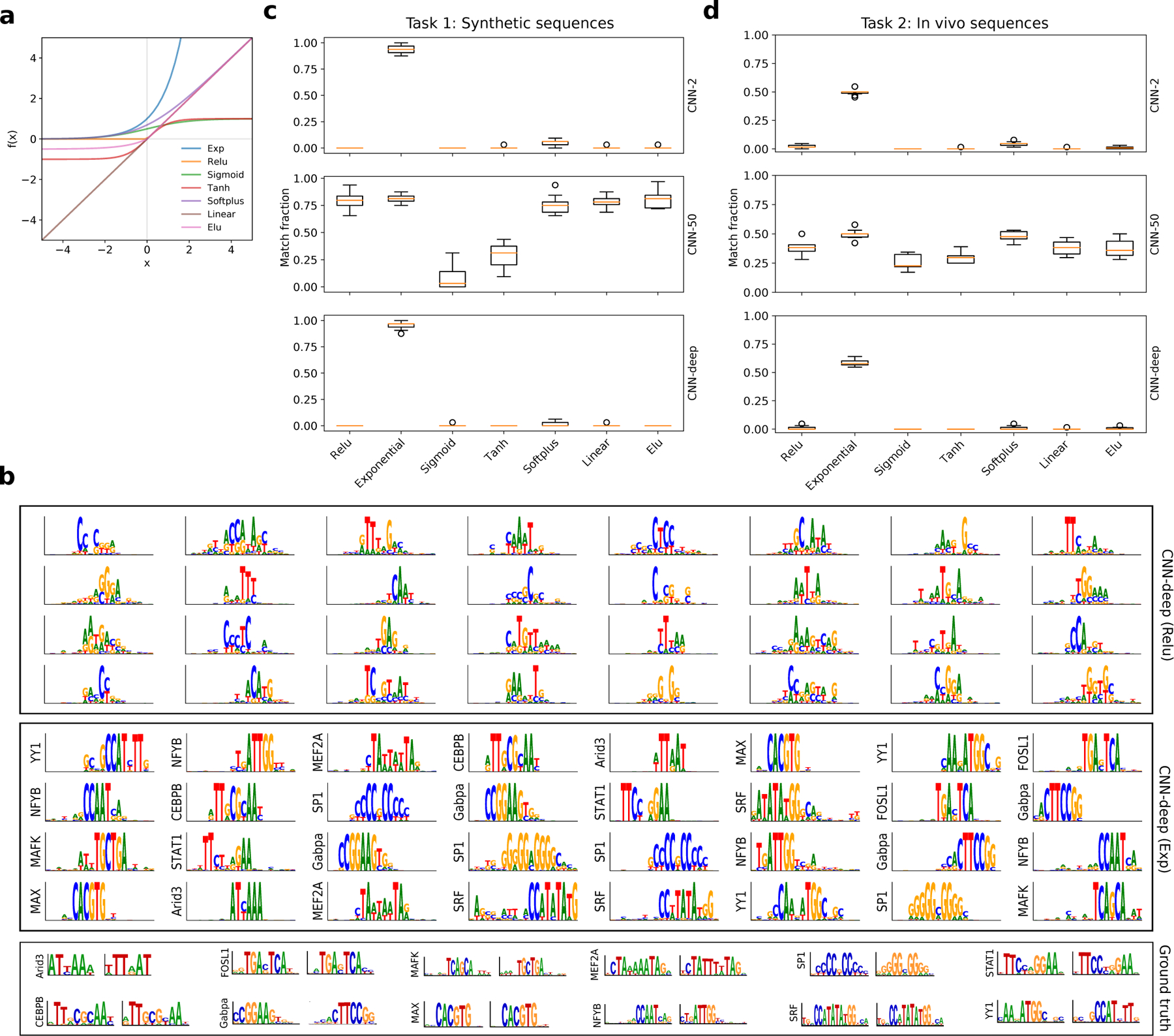
Motif representation performance. (a) Plot of various activation functions, including exponential (exp), relu, sigmoid, tanh, softplus, linear, and elu. (b) Sequence logos for first convolutional layer filters are shown for CNN-deep with relu activations (top) and exponential activations (middle). The sequence logo of the ground truth motifs and its reverse-complement for each transcription factor is shown at the bottom. The y-axis label on select filters represent a statistically significant match to a ground truth motif as determined by Tomtom with an E-value threshold of 0.1. None of the filters from CNN-deep with relu activations yield any hits to ground truth motifs. (c) Boxplot of the fraction of filters that match ground truth motifs for CNN-2 (top), CNN-50 (middle), and CNN-deep (bottom) with various first layer activations trained on synthetic sequences of Task 1. (d) Boxplot of the fraction of filters that match ground truth motifs for CNN-2 (top), CNN-50 (middle), and CNN-deep (bottom) with various first layer activations trained on real DNA sequences of Task 2. (c,d) Each boxplot represents the performance across 10 models with different random initialisations (box represents first and third quartile and the red line represents the median).

Exponential activations lead to improved motif representations.

To test the extent that CNN activations influence representation learning, we uniformly trained and tested various CNNs with different first layer activation functions on a multitask classification dataset from Ref.¹⁸, which we refer to as Task 1. The goal of Task 1 is to determine class membership based on the presence of transcription factor (TF) motifs embedded in random DNA sequences, where each TF motif represents a unique class. Using representation learning design concepts developed for CNNs with relu activations¹⁸, we explored 3 CNNs, namely CNN-2, CNN-50, and CNN-deep (see Methods). CNN-50 is designed with large max-pooling after the first of 2 convolutional layers to provide an inductive bias to learn “local” representations (i.e. whole motifs) in the first layer, while CNN-2 employs small max-pooling, which allows it to build “distributed” representations in a hierarchical manner by combining partial motifs learned in the first layer into whole representations in deeper layers. CNN-deep consists of 4 convolutional layers with small max-pooling, which is designed to build distributed motif representations.

The classification performances given by the area under the precision-recall curve (AUPR) on the held-out test set for Task 1 are more-or-less comparable across networks and activations (Supplementary Table 2). CNN-deep exhibits a slight overall edge while CNN-50 yields a slightly lower performance, with tanh and sigmoid activations yielding the poorest classification. Tweaking the initialisation strategy could presumably improve the performance²⁵ but was not explored here to maintain a systematic approach. To quantify how well representations learned in first layer filters match ground truth motifs, we visualised first layer filters using activation-based alignments^1,10 and employed Tomtom²⁶ to quantify the fraction of first layer filters that yield a statistically significant match to ground truth motifs (Fig. 1b). The filters in CNN-50, which are designed to learn whole motif representations with relu activations, were also able to capture ground truth motifs with other activations, the exceptions being sigmoid and tanh activations, which was expected given their poor classification performance (Fig. 1c). On the other hand, the CNNs designed to learn distributed representations, CNN-2 and CNN-deep, were unable to do so for most activation functions, with the exception being the exponential activation, which consistently yielded improved motif matches both quantitatively (Fig. 1c) and qualitatively (Supplementary Figs. 1 and 2). Notably, 36.6% of the filters of CNN-2 with softplus activations have a statistically significant match to some motif in the JASPAR database despite the vast majority of these being irrelevant for Task 1 (Supplementary Table 2). This highlights a potential pitfall that arises from over-interpreting filters that match an annotated motif from a motif database. Together, this demonstrates that exponential activations yield interpretable filters for CNNs, irrespective of max-pooling size and network depth without sacrificing performance.

Although the unbounded behaviour of the exponential could make the CNN activations diverge, in practice, there were no obvious issues with training (Supplementary Fig. 3), with convergence times that are similar to CNNs with relu activations and stable gradients throughout (Supplementary Fig. 4). In addition, we found CNNs with exponential activations are robust to standard initialisation strategies^27–30 (Supplementary Table 3) as well as over a large range of random normal initialisations with varying degrees of the standard deviation (Supplementary Table 4), albeit with decreased ability to learn robust motif representations for standard deviations that are far larger than what is typically employed (Supplementary Fig. 5).

Improved representation learning generalises to real DNA sequences.

We performed similar experiments on a modified DeepSea dataset², truncated to include only sequences with a peak called in at least one of 12 ChIP-seq experiments corresponding to those in Task 1 (see Methods), using augmented CNNs – doubling the number of parameters in each hidden layer – to account for the increased complexity of features in real DNA sequences³¹. We refer to this analysis as Task 2. The classification performance follows similar trends as Task 1 (Supplementary Table 2), albeit with a larger gap between CNN-deep and the shallower CNNs. Moreover, filter comparisons confirm that employing exponential activations consistently lead to more interpretable filters both visually (Supplementary Fig. 6) and quantitatively (Fig. 1d) for all CNNs, albeit with an overall decrease number of matches to relevant motifs, i.e. motifs in the JASPAR database that are associated with each TF. Consequently, filters that are dedicated to other TFs, such as GATA1, CTCF, GATA1-TAL1, ATF4, among many others, were not included as a motif match, despite being learned consistently across all random initialisations (see Supplementary Data).

Local function properties drive interpretability.

To understand the properties of the exponential activation that drive improved motif representations, we transformed sigmoid, tanh, and relu activations to emulate the exponential function locally near the origin (Supplementary Fig. 7, Supplementary Table 5). Indeed, these modified activations now yield comparable performance as the exponential activation for both synthetic sequences in Task 1 (Extended Data Fig. 1a) and real DNA sequences in Task 2 (Supplementary Fig. 8). As a control, we also modified the exponential activation to behave relu-like (Extended Data Fig. 1a). Since each modified activation can be decomposed to a shift- and a scale-transformation (Supplementary Table 5), we performed an ablation study, testing each transformation on its own. However, we could not identify a transformation that consistently worked well for all activations (Extended Data Fig. 1b). We also tested a relu activation modified to have a steep, linear slope of 400, we call super-relu, but found that high divergence alone does not lead to motif representations, resulting in performance metrics that closely resemble standard relu activations (Supplementary Table 2). In addition, we introduced and varied a multiplicative scaling factor for the inputs to the exponential. We found that performance was robust near a scaling factor of 1 but degrades rapidly for deviations greater than a factor of 2 in either direction (Supplementary Table 6, Supplementary Fig. 9). Taken together, this suggests that the divergence of the activation function alone is not sufficient, but rather, its combination with a shift from the origin provides a strong inductive bias to learn motif representations.

Exponential activations suppress background.

To better understand how the exponential activation processes input data, we compared the pre- and post-activations in the first layer of CNN-deep before and after training (Supplementary Fig. 10). We found that standard initialisations yield a low activity in first layer neurons with exponential activations, and as training progresses, parameters are tuned to activate just a few neurons to large values while background is maintained to low values. By contrast, standard initialisations applied to relu activations result in activity across half of the neurons. Surprisingly, the distribution of post-activations changes only slightly after training, shifting the mode to have a slight negative bias. This suggests that in addition to up-weighting signal, the CNN has to mainly down-weight the noise. During training, if the deeper layers learn to deal with noise, then there remains a low incentive to continue down-weighting the noise in the first layer filters, which would result in less interpretable filters.

Scanning exponentially activated filters localises motifs.

Since exponential activations suppress background and propagate signal, the first layer filter scans may be used to footprint motif instances along a sequence. Indeed, the first layer filter scans of CNN-deep with exponential activations yield crisp peaks at locations along the sequence where motifs were implanted (Extended Data Fig. 1c). The gold standard for motif scans are PWMs^32–34, which is a log-ratio of motif similarity given by the position probability matrix to background nucleotide levels (Extended Data Fig. 1d, middle row). Since we have ground truth for Task 1, we can quantify the motif localisation performance using the localisation AUROC (see Methods). Indeed, CNN-deep with exponential activations yield a localisation AUROC of 0.889±0.201, which is significantly greater than with relu activations (0.391±0.331, errors represent the standard deviation of the mean across all test sequences). The localisation AUROC for the ground truth PWMs is 0.884±0.252. This confirms that in ideal circumstances, i.e. knowing the ground truth motif and background frequencies, PWM scans are a powerful approach to footprint motifs along a sequence. In practice, motif activity may depend on flanking nucleotide context and can be nuanced from cell type to cell type³⁵. Moreover, PWM performance is sensitive to the choice of background frequencies³⁶. The appeal of CNNs is their ability to infer motif patterns and make predictions in an end-to-end manner.

Log-based activations actively suppress background.

Just as an exponential function provides a high sensitivity which the network can exploit to suppress background and propagate signal, a log₂ function of a PWM provides a high sensitivity to scale down background while maintaining signal. Both approaches serve to improve the signal-to-noise ratio. Hence, we tried a standard natural log as an activation for first layer filters of CNN-deep, but we found model training was quite unstable, presumably due to the large negative values that arise close to zero. To remedy this, we incorporated a relu activation after the log function, which we call log-relu combined with a strong L2-regularisation penalty of 0.2 (Supplementary Table 5). A strong L2-regularisation encourages parameters to stay close to zero, hence this provides a mechanism to drive background noise levels toward zero while maintaining signal above a value of 1, which adds a hefty L2 penalty that can only be outweighed by capturing discriminative patterns that minimises the loss, i.e. motifs. As a control, we applied the same L2-regularisation with CNN-deep with relu activations. The classification performance was accurate for both models (AUPR of 0.980±0.003 and 0.978±0.003 for log-relu and relu, respectively), but the motif representations were only interpretable for log-relu activations (Extended Data Fig. 1e). Together, this demonstrates that activations that provide a high-sensitivity to scale signal/background can improve learning motif representations.

CNNs that learn robust motif representations are more interpretable with attribution methods

Although filter visualisation is a powerful approach to assess learned representations from a CNN, they do not specify how decisions are made. Attribution methods aim to resolve this by identifying input features that are important for model predictions. To understand the role that the activation function plays in the efficacy of recovering biologically meaningful representations with attribution methods, we trained two CNNs, namely CNN-local and CNN-dist, on a synthetic regulatory classification task that serves to emulate the billboard model for cis-regulation^37,38. The goal of this binary classification task, which we refer to as Task 3, is to predict whether a DNA sequence contains at least 3 motifs sampled from a set of “core motifs” (positive class) versus motifs sampled from a background set (negative class). CNN-local is a shallow network with 2 hidden layers that is designed to learn interpretable filter representations with relu activations¹⁸, while CNN-dist is a deep network with 5 hidden layers that learn distributed representations of features. Since we have ground truth for which motifs were embedded and their positions in each sequence, we can test the efficacy of attribution methods by summarising the distribution of attribution scores at sequence locations with the embedded motifs and the without the embedded motifs using the interpretability AUROC and the interpretability AUPR (see Methods).

Better accuracy does not imply better interpretability.

Classification performance as measured by area-under the receiver-operating characteristic curve (AUC) is comparable between CNN-dist and CNN-local, with a slight edge in performance favouring CNN-dist (Fig. 2a, Supplementary Table 7). Using attribution scores given by saliency maps, i.e. gradients of predictions with respect to inputs, we find that CNN-local yields a slightly higher interpretability AUROC compared to CNN-dist across most activations functions, with the exception of the exponential activation (Fig. 2b); while, CNN-dist yields a slightly better performance under the AUPR metric (Fig. 2c). Each metric describes slightly different aspects of the attribution scores. AUROC captures the ability of the network to correctly predict the embedded motifs, while penalising spurious noise. Hence, CNN-local is less susceptible to attributing positions that are not associated with the ground truth motifs (lower false positives). AUPR considers false negative rates, and so the improved performance here suggests that CNN-dist is slightly better at capturing more ground truth patterns, while CNN-local tends to miss some ground truth patterns. One limitation of this study is that we are only accounting for ground truth motifs that are implanted in randomised sequence, not the spurious motifs that arise by chance, which contributes to label noise.

Figure 2.

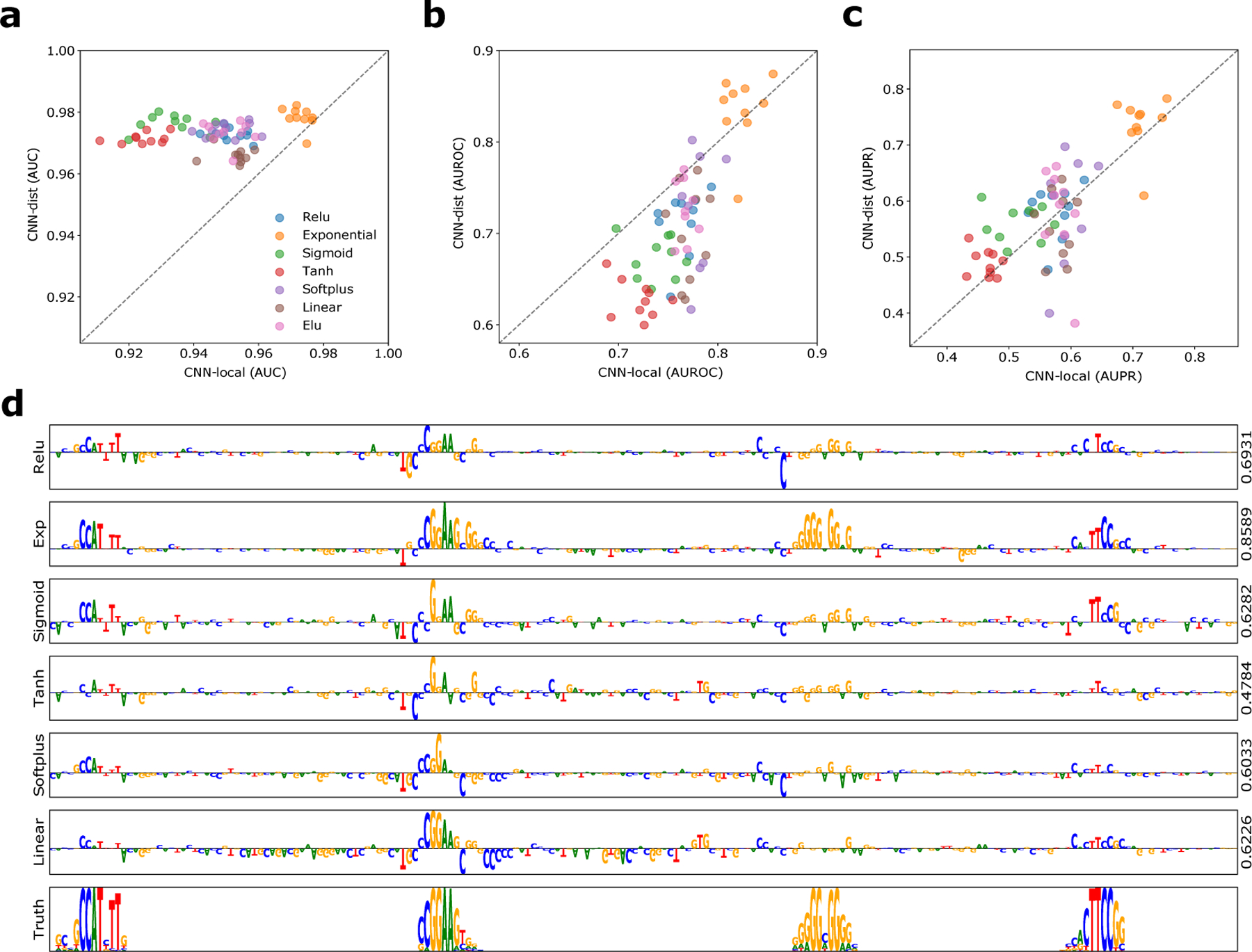
Interpretability performance of saliency maps. (a) Scatter plot of the classification AUC for CNN-dist versus CNN-local for different first layer activations (shown in a different colour), when trained with 10 different random intialisations. Scatter plot of the average (b) interpretability AUROC and (c) interpretability AUPR of saliency maps from test sequences generated from CNN-dist versus CNN-local for different activations (shown in a different colour). (d) Sequence logo of a saliency map for a representative test sequence generated with CNN-deep with different first layer activations (y-axis label). The right y-axis label shows the interpretability AUROC score. The sequence logo for the ground truth sequence model is shown at the bottom.

Interestingly CNN-dist with softplus and linear activations yields higher classification performance relative to CNN-local, but significantly lower interpretability under both interpretability metrics (Supplementary Table 7). This counters the common intuition that improved predictive models should better capture feature representations to explain the improved performances and suggests instead that predictive performance does not necessarily imply reliable interpretability with attribution methods. This discrepancy between accurate predictions and model interpretability has also been observed in computer vision³⁹. Strikingly, we find that exponential activations consistently lead to superior interpretability performance across all tested CNNs, both quantitatively (Figs. 2b,c) and qualitatively (Fig. 2d).

Several issues have been documented for saliency maps^8,40–42, and hence the poor performance may be a reflection of flawed methodology and not necessarily the model’s learned representations. We therefore compared the interpretability performance of different attribution methods, including in silico mutagenesis, integrated gradients, and DeepSHAP, and find that different attribution methods yield very different recovery of ground truth motifs (Extended Data Fig. 2 and Supplementary Table 8). The gold standard is in silico mutagenesis which consistently yields the most reliable attribution maps with DeepSHAP in second place. Irrespective of the attribution method used here, we find that CNNs that employ exponential activations significantly improve performance across all interpretability metrics compared with other activations.

Modified activations improve attribution scores.

Modifying activations, such as sigmoid, tanh, and relu, which all yield low interpretability performance, to behave exponential-like near the origin significantly improves the interpretability performance (Supplementary Figs. 11). Similarly, modifying the exponential to appear relu-like locally decreases interpretability performance. Together, this suggests the extent that CNN filters learn robust motif representations may be indicative of network’s interpretability performance with attribution methods.

Improved attribution interpretability generalises to in vivo sequences.

To validate that the improved representations with exponential activations generalises to real regulatory genomic sequences, we trained two Basset models on a multitask classification of chromatin accessibility sites, i.e. the Basset dataset¹, which we refer to as Task 4 (see Methods). Each Basset model consists of 3 convolutional layers followed by 2 fully-connected hidden layers with the only difference being the first layer activations, relu or exponential. Both Basset models yield very similar classification performance with an AUPR of 0.486±0.042 and 0.489±0.041 for relu and exponential activations, respectively. However, Basset with exponential activations evidently leads to more interpretable motif representations (Supplementary Fig. 12). Figure 3a shows an anecdotal example of a saliency map for an accessible DNA sequence in Fibroblast cells where a Basset model with exponential activations reveals 3 motifs – TCF4, NFIX, and HLF – which are all important regulators previously identified for chromatin accessibility^43–45. Similarly, exponential activations lead to more informative filters with a higher match fraction of 0.617 to the JASPAR database compared to 0.370 given by relu activations (see Supplementary data).

Figure 3.

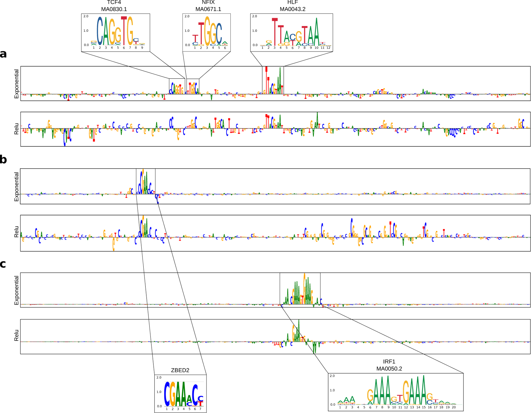
Attribution score comparison for real regulatory DNA sequences. Sequence logo of a saliency map generated for a representative test sequence from a CNN with exponential activations (top) and relu activations (bottom) trained on (a) Task 4 (DNase-seq peaks), (b) Task 5 (ZBED2 ChIP-seq peaks) and (c) Task 6 (IRF1 ChIP-seq peaks). The sequence logo of the known motifs are highlighted.

Consistent results are found for ResidualBind, a CNN originally employed for RNA-protein interactions⁴⁶, trained on ChIP-seq data for ZBED2 (Task 5) and IRF1 (Task 6). ResidualBind with relu and exponential activations yield comparable classification performance (AUROC on Task 5: 0.882 and 0.898 and Task 6: 0.985 and 0.982, respectively), but the attribution maps generated using a ResidualBind model with exponential activations are evidently more interpretable (Fig. 3b–c, Supplementary Figs. 13 and 14).

Discussion

A major draw of deep learning in genomics is their powerful ability to automatically learn features from the data that enable it to make accurate predictions. It is critical that we understand what features are learned to build trust in their predictions. Model interpretability is key to understanding these features. Deep CNNs, however, tend to learn distributed representations of sequence motifs that are far too complex to be processed by humans. While attribution methods identify input features that affect decision making, their scores tend to be noisy and difficult to interpret in practice. Here, we show that an exponential activation applied to the first layer is a powerful approach to encourage first layer filters to learn sequence motifs and also to improve the efficacy of attribution scores, revealing more interpretable representations.

One major consequence from this study raises the red flag that a CNN which yields high classification performance does not necessarily provide meaningful representations with attribution methods. Previous studies have focused on comparing representations from different attribution methods using only a single model⁸. Here, we show that different models, each with comparable classification performance, can yield significantly different representations with the same attribution methods. We believe CNNs that learn distributed representations may be learning a function that build noisier motifs, which may not necessarily impact classification performance but can result in poor interpertability. Investigating properties of the underlying function is important to address the root of this issue.

Variant effect prediction.

Scoring the functional impact of mutations is a promising application of deep learning in genomics. However, we must trust that the CNN is making reliable predictions. Testing model predictions on held-out test data is not sufficient to evaluate whether we can trust model predictions for single nucleotide mutations. We demonstrated that models that yield high classification performance can yield very low interpretability with first-order attribution methods, including in silico mutagenesis. While we do not elucidate all of the factors that underlie the discrepancy between model classification and interpretability, we identified a strong association that models that learn more robust representations of motifs in first layer filters lead to significantly improved interpretability with first-order attribution methods. We suspect that if a robust motif representation is learned anywhere in the network, then attribution methods will be reliable. Hence, verifying that a network has learned a strong motif representations can serve as a necessary (but not sufficient) quality control to ensure trust in attribution methods, including in silico mutagenesis. Since the representations of filters in deeper layers of a CNN are challenging to recover, enforcing that first layer filters learn strong motif representations can be achieved and easily verified with exponential (or equivalent) activations.

Trade off no more.

Previously, interpretability of first layer convolutional filters was seemingly at odds with classification performance, especially for deeper networks, which are more flexible in terms of the function classes that they can fit. Existing design principle for CNNs to learn interpretable motif representations tend to sacrifice network depth¹⁸, which, in general, leads to better classification performance. Here, we show that CNNs with exponential activations substantially improve motif representations in the first layer while not making any sacrifices in performance. Importantly, this trick can be applied to networks of any depth. Although not tested here, we believe that it could also improve filter interpretability in deeper layers to potentially capture motif-motif interactions. In practice, the exponential should probably only be applied to one layer for numerical stability. One possible solution is to instead employ an exponential equivalent that doesn’t diverge, such as a modified-sigmoid activation, to explore “interpretable” activations in multiple layers.

Methods

Data

Task 1.

Task 1 consists of a multitask classification dataset from Ref.¹⁸. This dataset consists of 30,000 synthetic DNA sequences embedded with known transcription factor motifs. Synthetic sequences, each 200 nucleotides long, were sampled from a uniform (i.e. equiprobable) sequence model implanted with 1 to 5 known TF motifs, randomly selected with replacement from a pool of 12 motifs, which include Arid3, CEBPB, FOSL1, Gabpa, MAFK, MAX, MEF2A, NFYB, SP1, SRF, STAT1, and YY1. Sequences were sampled once from a unique sequence model. This dataset makes a simplifying assumption that the only important pattern for a given binding event is the presence of a PWM-like motif in a sequence. The dataset is randomly split to a training, validation, and test set according to the fractions 0.7, 0.1, and 0.2, respectively.

Task 2.

Task 2 consists of a truncated version of the DeepSea dataset². The DeepSea dataset was reduced to 12 labels by removing sequences that did not correspond to 12 class labels defined in Supplementary Table 1 in Ref.¹⁸. This truncation only includes 12 labels that match the TFs in Task 1 in K562 cells. Sequences are 1000 nucleotides in length.

Task 3.

We generated 20,000 synthetic sequences each 200 nts long by embedding known motifs in specific combinations in a uniform sequence model. Positive class sequences were synthesised by sampling a sequence model embedded with 3 to 5 “core motifs” – randomly selected with replacement from a pool of 10 position frequency matrices, which include the forward and reverse-complement motifs for CEBPB, Gabpa, MAX, SP1, and YY1⁴⁷ – along a random sequence model. Negative class sequences were generated following the same steps with the exception that the pool of motifs include 100 non-overlapping “background motifs” from the JASPAR database⁴⁷. Background sequences can thus contain core motifs; however, it is unlikely to randomly draw motifs that resemble a positive regulatory code. We randomly combined synthetic sequences of the positive and negative class and randomly split the dataset into training, validation and test sets with a 0.7, 0.1, and 0.2 split, respectively.

Task 4.

Task 4 sequences are from the Basset dataset¹. This includes 164 DNase-seq datasets from ENCODE⁴⁸ and Roadmaps Epigenomics⁴⁹. The processed dataset consists of 1,879,982 training and 71,886 test sequences that are 600 nts long. Each sequence has an associated binary label vector corresponding to the presence of a statistically significant peak for each of the 164 cell types.

Tasks 5 and 6.

Processed ZBED2 and IRF1 ChIP-seq data for Tasks 5 and 6 were acquired from⁵⁰. Positive class sequences were defined as 400 nt sequences centred on ChIP-seq peaks in pancreatic ductal adenocarcinoma cells. Negative class sequences were defined as 200 nt sequences centred on peaks for H3K27ac ChIP-seq peaks that do not overlap with any positive peaks from the same cell type. We randomly subsampled the negative class sequences to balance the class labels. We randomly split the dataset into training, validation and test sets with a 0.7, 0.1, and 0.2 split, respectively. The total number of sequences is 4,902 and 3,892 for Tasks 5 and 6, respectively. We augmented the training data by generating reverse-complement sequences.

Models

Task 1.

CNN-2, CNN-50, and CNN-deep take as input a 1-dimensional one-hot-encoded sequence with 4 channels, one for each nucleotide (A, C, G, T), and have a fully-connected (dense) output layer with 12 neurons that use sigmoid activations. The hidden layers for each model are:

1. CNN-2

1. convolution (32 filters, size 19, activation) max-pooling (size 2)

2. convolution (124 filters, size 5, relu) max-pooling (size 50)

3. fully-connected layer (512 units, relu)

2. CNN-50

1. convolution (32 filters, size 19, activation) max-pooling (size 50)

2. convolution (124 filters, size 5, relu) max-pooling (size 2)

3. fully-connected layer (512 units, relu)

3. CNN-deep

1. convolution (32 filters, size 19, activation)

2. convolution (48 filters, size 9, relu) max-pooling (size 4)

3. convolution (96 filters, size 6, relu) max-pooling (size 4)

4. convolution (128 filters, size 4, relu) max-pooling (size 3)

5. fully-connected layer (512 units, relu)

All models incorporate batch normalisation⁵¹ in each hidden layer prior to the nonlinear activation; dropout⁵² with probabilities corresponding to 0.1 (layer 1), 0.1 (layer 2), 0.5 (layer 3) for CNN-2 and CNN-50; and 0.1 (layer 1), 0.2 (layer 2), 0.3 (layer 3), 0.4 (layer 4), 0.5 (layer 5) for CNN-deep; and L2-regularisation on all parameters in the network with a strength equal to 1e-6, unless stated otherwise.

Task 2.

Same models as Task 1 but with augmented hidden layers, multiplying the number of filters or hidden units by a factor of 2. Note that the inputs to the models also change from 200 nt to 1000 nt.

Task 3.

We designed two CNNs, namely CNN-local and CNN-deep, to learn “local” representations (whole motifs) and “distributed” representations (partial motifs), respectively. Both take as input a 1-dimensional one-hot-encoded sequence (200 nt) and have a fully-connected (dense) output layer with a single sigmoid activation. The hidden layers for each model are:

1. CNN-local

1. convolution (24 filters, size 19, activation) max-pooling (size 50)

2. fully-connected layer (96 units, relu)

2. CNN-dist

1. convolution (24 filters, size 7, activation)

2. convolution (32 filters, size 9, relu) max-pooling (size 3)

3. convolution (48 filters, size 6, relu) max-pooling (size 4)

4. convolution (64 filters, size 4, relu) max-pooling (size 3)

5. fully-connected layer (96 units, relu)

We incorporate batch normalisation in each hidden layer prior to the nonlinear activation; dropout with probabilities corresponding to: CNN-local (layer1 0.1, layer2 0.5) and CNN-deep (layer1 0.1, layer2 0.2, layer3 0.3, layer4 0.4, layer5 0.5); and L2-regularisation on all parameters in the network with a strength equal to 1e-6.

Task 4.

We replicated a Basset-like model that takes as input a 1-dimensional one-hot-encoded sequence (600 nt) and have a fully-connected (dense) output layer with 164 units with sigmoid activations. The hidden layers for each model are:

1. Basset

1. convolution (300 filters, size 19, activation) max-pooling (size 3)

2. convolution (200 filters, size 11, relu) max-pooling (size 4)

3. convolution (200 filters, size 7, relu) max-pooling (size 4)

4. fully-connected (1000 units, relu)

5. fully-connected (1000 units, relu)

We incorporate batch normalisation in each hidden layer prior to the nonlinear activation; dropout with probabilities corresponding to: 0.2, 0.2, 0.2, 0.5 and 0.5; and L2-regularisation on all parameters in the network with a strength equal to 1e-6.

Tasks 5 and 6.

We employed a ResidualBind-like model to classify positive-label DNA sequences about ChIP-seq peaks for ZBED2 (Task 5) and IRF1 (Task 6) in pancreatic ductal adenocarcinoma cells versus negative-label sequences about ChIP-seq peaks for H3K27ac marks within the same cell-type (nonoverlapping peaks with the TFs)⁵⁰. The model takes as input one-hot encoded sequence (400 nt) and have a fully-connected layer to a single unit with sigmoid activations. The hidden layers are:

1. Residualbind

1. convolution (24 filters, size 19, activation) residual block max-pooling (size 10)

2. convolution (48 filters, size 7, relu) max-pooling (size 5)

3. convolution (64 filters, size 7, relu) max-pooling (size 4)

4. fully-connected (96 units, relu)

The residual block consists of a convolutional layer with filter size 5, followed by batch normalisation, relu activation, dropout with a probability of 0.1, convolutional layer with filter size 5, batch normalisation, and a element-wise sum with the inputs to the residual block, a so-called skipped connection, followed by a relu activation, and dropout with a probability of 0.2. For each hidden layer, we incorporate batch normalisation⁵¹ and dropout⁵² with probabilities corresponding to: 0.1, 0.3, 0.4, and 0.5.

Training.

We uniformly trained each model by minimising the binary cross-entropy loss function with mini-batch stochastic gradient descent (100 sequences) for 100 epochs with Adam updates using default parameters⁵³. We decayed the learning rate which started at 0.001, and when the performance metric that was monitored (AUPR for Tasks 1, 2, 4; AUROC for Tasks 3, 5, 6) did not improve for 5 epochs, the learning rate was decayed by a factor 0.3. All reported performance metrics are drawn from the test set using the model parameters which yielded the highest performance metric on the validation set. Each model was trained (10 times for Tasks 1–3 and once for Task 4–6) with different random initialisations according to Ref.²⁷.

Filter analysis

Filter visualisation.

To visualise first layer filters, we scanned each filter across every sequence in the test set. Sequences whose maximum activation was less than a cutoff of 50% of the maximum possible activation achievable for that filter in the test set were removed^1,10. A subsequence the size of the filter centred about the max activation for each remaining sequence and assembled into an alignment. Subsequences that are shorter than the filter size due to their max activation being too close to the ends of the sequence were also discarded. A position frequency matrix was then created from the alignment and converted to a sequence logo using Logomaker⁵⁴. The motif representations were largely not sensitive to the activation threshold (Supplementary Fig. 15), with only a slight increase in motif matches for CNN-deep with relu activations for higher activation thresholds. On the other hand, exponential activations decrease presumably due to the reduced sequence diversity in the alignment when high thresholds are applied.

Quantitative motif comparison.

The interpretability of each filter was assessed using the Tomtom motif comparison search tool²⁶ to determine statistically significant matches to the 2016 JASPAR vertebrates database⁴⁷, with the exception of Grembl, for which many filters yielded a statistically significant match, despite visually appearing non-informative. Since the ground truth motifs are available for our synthetic dataset, we can test whether the CNNs have captured relevant motifs. Tomtom was employed with an E-value threshold of 0.1.

Motif localisation analysis.

The performance of locating motifs along a given sequence with motif scans was quantified by segmenting the sequence into regions that have the implanted motif or do not. This was determined by calculating the information content of the sequence model used to generate the synthetic sequence and segmenting ground truth from background according to an information content threshold greater than zero. A buffer size of 10 nts was added to the boundaries of each embedded motif, because motif positions within filters are not necessarily centred. The max filter scan score was given for each segmented region with a label of one for ground truth regions and a label of zero otherwise. The positive and negative label scores were aggregated across all test sequences and the AUROC was calculated.

Attribution analysis

Attribution methods.

To test interpretability of trained models, we generate attribution scores by employing saliency maps⁶, in silico mutagenesis^1,2,10, integrated gradients⁷, and DeepSHAP⁹. Saliency maps were calculated by computing the gradients of the predictions with respect to the inputs. Integrated gradients were calculated by adding the saliency maps generated from 20 sequences that linearly interpolate between a reference sequence and the query sequence. We average the integrated gradients score across 10 different reference sequences generated from random shuffles of the query sequence. For DeepSHAP, we used the package from Ref.⁹, and averaged the attribution scores across 10 different randomly shuffled reference sequences. We found that 10 randomly shuffled reference sequences marked the elbow point where the inclusion of additional sequences only provided a marginal improvement in performance (Supplementary Fig. 16). Saliency maps, integrated gradients, and DeepShap scores were multiplied by the query sequence (times inputs). In silico mutagenesis was calculated by generating new sequences with all possible single nucleotide mutations of a sequence and monitoring the change in prediction compared to wildtype. In silico mutagenesis scores were reduced to a single score for each position by calculating the L2-norm of the mutagenesis scores across nucleotides for each position. All attribution maps were visualised as a sequence logo using Logomaker⁵⁴.

Quantifying interpretability.

Since we have the ground truth of embedded motif locations in each sequence, we can test the efficacy of attribution scores. To quantify the interpretability of a given attribution map, we calculate the area under the receiver-operating characteristic curve (AUROC) and the area under the precision-recall curve (AUPR), comparing the distribution of attribution scores where ground truth motifs have been implanted (positive class) and the distribution of attribution scores at positions not associated with any ground truth motifs (negative class). Specifically, we first multiply the attribution scores (S_ij) and the input sequence (X_ij) and reduce the dimensions to get a single score per position, according to C_i =∑_j S_ijX_ij, where j is the alphabet and i is the position. We then calculate the information of the sequence model, M_ij, according to I_i = log₂ 4−_∑j M_ij log₂ M_ij. Positions that are given a positive label are defined by I_i > 0.01, while other positions are given a negative label. The AUROC and AUPR is then calculated separately for each sequence using the distribution of C_i at positive label positions against negative label positions.

Extended Data

Extended Data Figure 1.

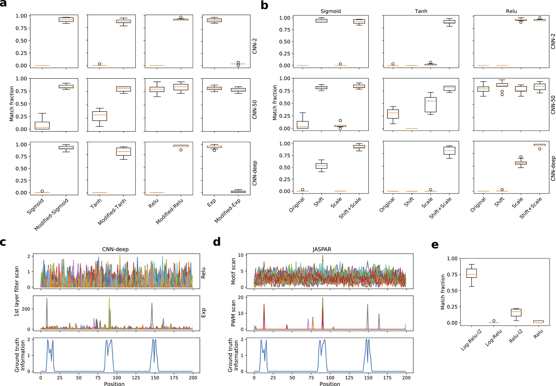
Task 1 motif representations for CNNs with modified activations. (a) Boxplot of the fraction of filters that match ground truth motifs for different CNNs with traditional and modified activations. (b) Boxplot of the fraction of filters that match ground truth motifs for an ablation study of transformations for modified activations. (c) First layer filter scans from CNN-deep with relu activations (top) and exponential activations (middle). Each colour represents a different filter. (d) Motif scans (top) and PWM scans (middle) using ground truth motifs and their reverse-complements (each colour represents a different filter scan). Negative PWM scan values were rectified to a value of zero. (c, d) The information content of the sequence model used to generate the synthetic sequence (ground truth), which has 3 embedded motifs centred at positions 15, 85, and 150, is shown at the bottom. (e) Boxplot of the fraction of filters that match ground truth motifs for CNN-deep with various activations: log activations trained with and without L2-regularisation (Log-Relu-L2 and Log-Relu, respectively) and relu activations with and without L2-regularisation. (a, b, e) Each boxplot represents the performance across 10 models trained with different random intialisations (box represents first and third quartile and the red line represents the median).

Extended Data Figure 2.

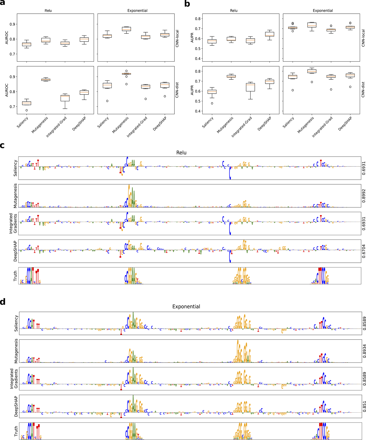
Interpretability performance comparison of different attribution methods. Boxplots of the interpretability AUROC (a) and AUPR (b) for CNN-local (top) and CNN-dist (bottom) with relu activations (left) and exponential activations (right) for different attribution methods. Each boxplot represents the performance across 10 models trained with different random intialisations (box represents first and third quartile and the red line represents the median). Sequence logo of a saliency map for a Task 3 test sequence generated with different attribution methods for CNN-deep with relu activations (c) and exponential activations (d). The right y-axis label shows the interpretability AUROC score. (c-d) The sequence logo for the ground truth sequence model is shown at the bottom.

Data availability

Data for Tasks 1, 3, 5, and 6 and code to generate data for Tasks 2 is available at: https://doi.org/10.5281/zenodo.4301062. Data for Task 4 is available via Ref.¹.

References

- 1.Kelley DR, Snoek J & Rinn JL Basset: learning the regulatory code of the accessible genome with deep convolutional neural networks. Genome Res 26, 990–9 (2016). [DOI] [PMC free article] [PubMed] [Google Scholar]
- 2.Zhou J & Troyanskaya OG Predicting effects of noncoding variants with deep learning–based sequence model. Nat. Methods 12, 931–4 (2015). [DOI] [PMC free article] [PubMed] [Google Scholar]
- 3.Jaganathan K et al. Predicting splicing from primary sequence with deep learning. Cell 176, 535–48 (2019). [DOI] [PubMed] [Google Scholar]
- 4.Bogard N, Linder J, Rosenberg AB & Seelig G A deep neural network for predicting and engineering alternative polyadenylation. Cell 178, 91–106 (2019). [DOI] [PMC free article] [PubMed] [Google Scholar]
- 5.Koo PK & Ploenzke M Deep learning for inferring transcription factor binding sites. Curr. Opin. Syst. Biol 19 (2020). [DOI] [PMC free article] [PubMed] [Google Scholar]
- 6.Simonyan K, Vedaldi A & Zisserman A Deep inside convolutional networks: Visualising image classification models and saliency maps. arXiv 1312.6034 (2013).
- 7.Sundararajan M, Taly A & Yan Q Axiomatic attribution for deep networks. In International Conference on Machine Learning, vol. 70, 3319–3328 (2017). [Google Scholar]
- 8.Shrikumar A, Greenside P & Kundaje A Learning important features through propagating activation differences. In International Conference on Machine Learning, vol. 70, 3145–3153 (2017). [Google Scholar]
- 9.Lundberg S & Lee S A unified approach to interpreting model predictions. In Advances in Neural Information Processing Systems, vol. 4765–4774 (2017). [Google Scholar]
- 10.Alipanahi B, Delong A, Weirauch MT & Frey BJ Predicting the sequence specificities of dna-and rna-binding proteins by deep learning. Nat. Biotechnol 33, 831–8 (2015). [DOI] [PubMed] [Google Scholar]
- 11.Selvaraju R et al. Grad-cam: Visual explanations from deep networks via gradient-based localization In IEEE International Conference on Computer Vision, 618–626 (2017). [Google Scholar]
- 12.Jha A, Aicher JK, Gazzara MR, Singh D & Barash Y Enhanced integrated gradients: improving interpretability of deep learning models using splicing codes as a case study. Genome Biol 21, 1–22 (2020). [DOI] [PMC free article] [PubMed] [Google Scholar]
- 13.Erhan D, Bengio Y, Courville A & Vincent P Visualizing higher-layer features of a deep network. In ICML Workshop on Learning Feature Hierarchies, vol. 1341 (2009). [Google Scholar]
- 14.Yosinski J, Clune J, Nguyen A, Fuchs T & Lipson H Understanding neural networks through deep visualization. arXiv 1506.06579 (2015).
- 15.Lanchantin J, Singh R, Lin Z & Qi Y Deep motif: Visualizing genomic sequence classifications. arXiv 1605.01133 (2016).
- 16.Shrikumar A et al. Tf-modisco v0. 4.4. 2-alpha. arXiv 1811.00416 (2018).
- 17.Koo P, Qian S, Kaplun G, Volf V & Kalimeris D Robust neural networks are more interpretable for genomics. bioRxiv 657437 (2019). [Google Scholar]
- 18.Koo PK & Eddy SR Representation learning of genomic sequence motifs with convolutional neural networks. PLoS Comput. Biol 15 (2019). [DOI] [PMC free article] [PubMed] [Google Scholar]
- 19.Ploenzke M & Irizarry R Interpretable convolution methods for learning genomic sequence motifs. bioRxiv 411934 (2018). [Google Scholar]
- 20.Raghu M, Poole B, Kleinberg J, Ganguli S & Sohl-Dickstein J On the expressive power of deep neural networks. arXiv 1606.05336 (2016). [Google Scholar]
- 21.Kelley D et al. Sequential regulatory activity prediction across chromosomes with convolutional neural networks. Genome Res 28, 739–50 (2018). [DOI] [PMC free article] [PubMed] [Google Scholar]
- 22.Nair V & Hinton GE Rectified linear units improve restricted boltzmann machines. In International Conference on Machine Learning, 807–814 (2010). [Google Scholar]
- 23.Dugas C, Bengio Y, Belisle F, Nadeau C & Garcia R Incorporating second-order functional knowledge for better option pricing. In Advances in Neural Information Processing Systems, 472–478 (2001). [Google Scholar]
- 24.Clevert DA, Unterthiner T & Hochreiter S Fast and accurate deep network learning by exponential linear units (elus). arXiv 1511.07289 (2015). [Google Scholar]
- 25.Pennington J, Schoenholz S & Ganguli S Resurrecting the sigmoid in deep learning through dynamical isometry: theory and practice. In Advances in Neural Information Processing Systems, 4785–4795 (2017). [Google Scholar]
- 26.Gupta S, Stamatoyannopoulos JA, Bailey TL & Noble WS Quantifying similarity between motifs. Genome Biol 8 (2007). [DOI] [PMC free article] [PubMed] [Google Scholar]
- 27.Glorot X & Bengio Y Understanding the difficulty of training deep feedforward neural networks. In Aistats, vol. 9, 249–256 (2010). [Google Scholar]
- 28.He K, Zhang X, Ren S & Sun J Delving deep into rectifiers: Surpassing human-level performance on imagenet classification. In IEEE International Conference on Computer Vision, 1026–1034 (2015). [Google Scholar]
- 29.LeCun YA, Bottou L, Orr GB & Müller K-R Efficient backprop. In Neural networks: Tricks of the trade, 9–48 (Springer, 2012). [Google Scholar]
- 30.Klambauer G, Unterthiner T, Mayr A & Hochreiter S Self-normalizing neural networks. In Advances in Neural Information Processing Systems, 971–980 (2017). [Google Scholar]
- 31.Siggers T & Gordan R Protein–DNA binding: complexities and multi-protein codes. Nucleic Acids Res 42, 2099–2111 (2014). [DOI] [PMC free article] [PubMed] [Google Scholar]
- 32.Stormo GD, Schneider TD, Gold L & Ehrenfeucht A Use of the ‘perceptron’ algorithm to distinguish translational initiation sites in e. coli. Nucleic Acids Res 10, 2997–3011 (1982). [DOI] [PMC free article] [PubMed] [Google Scholar]
- 33.Heinz S et al. “simple combinations of lineage-determining transcription factors prime cis-regulatory elements required for macrophage and b cell identities. Mol. Cell 38, 576–589 (2010). [DOI] [PMC free article] [PubMed] [Google Scholar]
- 34.Grant CE, Bailey TL & Noble WS Fimo: scanning for occurrences of a given motif. Bioinformatics 27, 1017–8 (2011). [DOI] [PMC free article] [PubMed] [Google Scholar]
- 35.Inukai S, Kock KH & Bulyk ML Transcription factor–dna binding: beyond binding site motifs. Curr. Opin. Genet. & Dev 43, 110–119 (2017). [DOI] [PMC free article] [PubMed] [Google Scholar]
- 36.Simcha D, Price ND & Geman D The limits of de novo dna motif discovery. PLoS One 7 (2012). [DOI] [PMC free article] [PubMed] [Google Scholar]
- 37.Kulkarni MM & Arnosti DN Information display by transcriptional enhancers. Development 130, 6569–75 (2003). [DOI] [PubMed] [Google Scholar]
- 38.Slattery M et al. Absence of a simple code: how transcription factors read the genome. Trends Biochem. Sci 39, 381–99 (2014). [DOI] [PMC free article] [PubMed] [Google Scholar]
- 39.Tsipras D, Santurkar S, Engstrom L, Turner A & Madry A Robustness may be at odds with accuracy. arXiv 1805.12152 (2018).
- 40.Adebayo J et al. Sanity checks for saliency maps. In Advances in Neural Information Processing Systems, 9505–9515 (2018).
- 41.Sixt L, Granz M & Landgraf T When explanations lie: Why modified bp attribution fails. arXiv 1912.09818 (2019).
- 42.Adebayo J, Gilmer J, Goodfellow I & Kim B Local explanation methods for deep neural networks lack sensitivity to parameter values. arXiv 1810.03307 (2018).
- 43.Piper M, Gronostajski R & Messina G Nuclear factor one x in development and disease. Trends Cell Biol 29, 20–30 (2019). [DOI] [PubMed] [Google Scholar]
- 44.Forrest MP et al. The emerging roles of tcf4 in disease and development. Trends Mol. Medicine 20, 322–331 (2014). [DOI] [PubMed] [Google Scholar]
- 45.Wei B et al. A protein activity assay to measure global transcription factor activity reveals determinants of chromatin accessibility. Nat. Biotechnol 36, 521–529 (2018). [DOI] [PubMed] [Google Scholar]
- 46.Koo PK, Ploenzke M, Anand P, Paul S & Majdandzic A Global importance analysis: A method to quantify importance of genomic features in deep neural networks. bioRxiv 288068 (2020). [DOI] [PMC free article] [PubMed]
- 47.Mathelier A et al. Jaspar 2016: a major expansion and update of the open-access database of transcription factor binding profiles. Nucleic Acids Res 44, D110–D115 (2016). [DOI] [PMC free article] [PubMed] [Google Scholar]
- 48.Consortium EP et al. An integrated encyclopedia of DNA elements in the human genome. Nature 489, 57–74 (2012). [DOI] [PMC free article] [PubMed] [Google Scholar]
- 49.Kundaje A et al. Integrative analysis of 111 reference human epigenomes. Nature 518, 317–330 (2015). [DOI] [PMC free article] [PubMed] [Google Scholar]
- 50.Somerville TD et al. Zbed2 is an antagonist of interferon regulatory factor 1 and modifies cell identity in pancreatic cancer. Proc. Natl. Acad. Sci (2020). [DOI] [PMC free article] [PubMed]
- 51.Ioffe S & Szegedy C Batch normalization: Accelerating deep network training by reducing internal covariate shift. arXiv 1502.03167 (2015).
- 52.Srivastava N, Hinton GE, Krizhevsky A, Sutskever I & Salakhutdinov R Dropout: a simple way to prevent neural networks from overfitting. J. Mach. Learn. Res 15, 1929–1958 (2014). [Google Scholar]
- 53.Kingma D & Ba J Adam: A method for stochastic optimization. arXiv 1412.6980 (2014).
- 54.Tareen A & Kinney J Logomaker: Beautiful sequence logos in python. bioRxiv 635029 (2019). [DOI] [PMC free article] [PubMed]
Associated Data
This section collects any data citations, data availability statements, or supplementary materials included in this article.
Supplementary Materials
Data Availability Statement