Word embeddings and deep learning for location prediction: tracking Coronavirus from British and American tweets

Abstract

With the propagation of the Coronavirus pandemic, current trends on determining its individual and societal impacts become increasingly important. Recent researches grant special attention to the Coronavirus social networks infodemic to study such impacts. For this aim, we think that applying a geolocation process is crucial before proceeding to the infodemic management. In fact, the spread of reported events and actualities on social networks makes the identification of infected areas or locations of the information owners more challenging especially at a state level. In this paper, we focus on linguistic features to encode regional variations from short and noisy texts such as tweets to track this disease. We pay particular attention to contextual information for a better encoding of these features. We refer to some neural network-based models to capture relationships between words according to their contexts. Being examples of these models, we evaluate some word embedding ones to determine the most effective features’ combination that has more spatial evidence. Then, we ensure a sequential modeling of words for a better understanding of contextual information using recurrent neural networks. Without defining restricted sets of local words in relation to the Coronavirus disease, our framework called DeepGeoloc demonstrates its ability to geolocate both tweets and twitterers. It also makes it possible to capture geosemantics of nonlocal words and to delimit the sparse use of local ones particularly in retweets and reported events. Compared to some baselines, DeepGeoloc achieved competitive results. It also proves its scalability to handle large amounts of data and to geolocate new tweets even those describing new topics in relation to this disease.

Introduction

Over the last decade, geographic information that can be extracted from location-based social networks (LBSN) highlighted its importance for multiple applications like socio-environmental studies (Beldad and Kusumadewi (2015); Jiang and Ren (2019); Larson et al. (2019)), sentiment analysis (Singh et al. (2018); Martinez et al. (2018)) disaster management (De Albuquerque et al. (2015); Ahmouda et al. (2018)), etc. Being a popular LBSN, Twitter receives an average of 500 million tweets from 152 million daily active users. By analyzing geotags that are associated with tweets, it becomes easier to determine tweets’ contexts. These latter describe human activities and interests which are in turn often linked to space (Lingad et al. 2013; Ao et al. 2014; Ma et al. 2020). In this direction and with the spread of the Coronavirus (COVID-19), understanding twitterers’ reactions regarding this disease is primordial to hedge their panic as far as the Ebola outburst (Tran and Lee (2016)). In addition, regional emergency interventions can be planned more effectively after determining current locations of users and their movements in the areas of contagion. More general concerns like impacts of Coronavirus on economy, social mobility and policy can be studied from geotagged tweets (Jiang et al. 2020; Xu et al. 2020). Despite the importance of spatial dimensions, prior studies demonstrate that the rate of geolocated tweets is less than 0.85% (Cheng et al. 2010; Priedhorsky et al. 2014; Hawelka et al. 2014). We explain this low rate by the optional adding of locations when creating a Twitter account or when sharing tweets. In addition, due to security issues or unaware preferences, even declared locations can be fictitious, invalid or ambiguous (Hecht et al. 2011; Chang et al. 2012; Zhao and Sui 2017). In relation to Coronavirus, such limitations make the tracking of this pandemic more challenging considering its wide global spread. In the light of these constraints, multiple works are established to extract geographical information from non-geotagged tweets. While some works are developed to determine a tweet’s location, the rest tends to estimate a user’s home location. For the second class, a set of tweets that are shared by the same user are analyzed at a time. For both geolocation subproblems, the location of a given tweet is estimated based on the geographical distribution of its words. From a deep study of these works, we find that they commonly share some drawbacks so they might be less adequate to manage the Coronavirus infodemic. We think that the proposed solutions which are mostly grid-based are less adequate to capture geographic boundaries leading then to a lack of geolocation accuracy. In addition, these solutions are designed to treat words in a tweet as independent sources of spatial evidence. Thus, encoded information by the whole tweet can be less effective. Finally, the definition of restricted sets of local words and the absence of dedicated pre-processing methods decrease their performance against the diversity of writing styles that characterizes social networks particularly when reporting new and global topics such as the spread of Coronavirus. Starting from these limitations, we think that we have to approach the geolocation task from a more generic perspective. Without defining a limited set of local words in relation to Coronavirus, we have to develop a strategy to estimate locations for tweets that contain even noisy texts and OOVs (out-of-vocabulary). To do this, we find that deriving geographical knowledge from linguistic features is efficient. While we agree that dialects, slang terms and regional accents can be effective to track this disease, we suppose that their utility is conditioned by taking into account topic’s dispersion on social networks. Otherwise, considering these features as inherent components in texts with potential spatial indications, they may serve to distinguish between different usages and forms of words and then to better differentiate one region from another. We also suppose that they enable supporting the diversity of writing styles when describing the same topic by users from the same region or from nearby regions. Since these features necessitate the encoded contextual information to comprise tweets’ contents and thus to infer their geographical appurtenance, we think that word embedding models can be effective solutions. We refer also to RNNs (recurrent neural networks) in order to maintain word order and to ensure sequential modeling of words in tweets on the one hand. On the other hand, we explore such neural networks to distinguish between local words and nonlocal ones regarding the contexts where they appear.

In this paper, our contributions to track Coronavirus from tweets are the following:

• We foremost proceed to a real-time collection of a set of English geotagged tweets by specifying a set of keywords that describes the Coronavirus topic. These tweets are retrieved from the UK and the USA so that we can evaluate the performance of our model to distinguish between two English variants. We make our code and the resulting corpus available for download.

• We evaluate some word embedding models in order to determine which combination of linguistic features encoded in English tweets has more spatial indications. Another model is also involved in making the treatment of misspelled forms and OOVs possible.

• Given that a word sense may vary from one region to another, we propose a WSD (word sense disambiguation) model. The intuition behind this model is to determine correct senses of words (nonlocal) and then to capture their geosemantic distribution. To do this, we refer to RNNs and precisely to bidirectional LSTMs (long short-term memory) for a sequential modeling of tweets’ words.

• Considering the unlimited dispersion of words on Twitter that describe the Coronavirus topic, we propose an attention model that assigns minimal importance to words that can disturb our geolocation results. These words (local) may be less important when contained in tweets that are shared from different regions. Like the WSD model, the latter is based on a bidirectional LSTM.

• By developing a distributed version based on a set of Apache frameworks, we make our geolocation strategy scalable enough to treat huge amounts of tweets in acceptable deadlines. This is especially advantageous when training word embedding models that encode subword information.

• We demonstrate that our framework DeepGeoloc yields better geolocation accuracy than state-of-the art approaches when applied on our Coronavirus corpus. In addition, its performance is guaranteed even when treating new tweets written in a single English variant as we deal with linguistic features instead of a delimited set of words or topics’ descriptions.

The remainder of this paper is organized as follows: In Sect. 2, we give an overview of prior work elaborated for the geolocation of tweets and twitterers. Then, our research objectives are detailed in Sect. 3. Section 4 elaborates on our research context where we describe some neural network-based models as candidate solutions to approach the geolocation task. Based on these models, the architecture of DeepGeoloc is detailed in Sect. 5. An experimental design for DeepGeoloc and an analysis of obtained results are described, respectively, in Sects. 6 and  7. Finally, Sect. 8 presents the conclusion and future scope of work.

Related work

We restrict our study to conducted works that rely purely on text content which makes the geolocation task more defiant especially when treating short texts like tweets. Note that some tendencies toward the resolution of this task by including additional metadata (user’s credibility, user’s social interactions, temporal effects, etc.) are also emergent but not discussed in this paper. The set of studied works adopts the assumption that there is a relation between a tweet’s content and the location from which it is shared. For more details, frequently used words in a given region can be descriptors for that region. Hence, checking the presence of such words in tweets can be effective to determine user’s mobility (tweet geolocation) or user’s home (twitterer geolocation).

Tweet geolocation

Since the encoded information in a single tweet is limited, the set of established approaches to geolocate tweets remains reduced. For instance, Melo and Martins (2015) propose a supervised classification-based approach where training tweets are represented by feature vectors. These latter are composed of weights of a tweet’s words. To do this, the TF-IDF (term frequency-inverse document frequency) weighting measure is applied. A recursive subdivision of the earth’s surface into curvilinear and quadrilateral regions is then performed where each cell corresponds to a region with a set of representative textual descriptions. As for the classification process, support vector machine (SVM) models are selected to infer new documents’ locations based on their similarities with the defined set of classes (cells). The application of TF-IDF for a limited period of time was also approached in (Paraskevopoulos and Palpanas 2015). For example, a location l of a given tweet T that is shared during [$t_i$, $t_n$] can be estimated by measuring its similarity with other geolocated tweets that are shared during the same time interval. Since the encoded information by a single tweet is relatively limited, it may be useful to treat this entry with a certain amount of redundancy. This reasoning is adopted in (Priedhorsky et al. 2014). Firstly, a GMM (Gaussian mixture model) is created for each n-gram $w_j$ whose occurrence rate exceeds a fixed threshold. This model determines the probability distribution of the n-gram in question in the set of the training tweets: g(l| $w_j$). Then, the weighted sum of the corresponding GMMs is used to estimate the geolocation of new tweets. Unlike (Priedhorsky et al. 2014), Lee et al. (2014) find that the value carried by a tweet is not limited to its size but rather to indications of its words. They believe that the combination of location and its semantic descriptions can better serve the geolocation of tweets. In this regard, they refer to Foursquare1 as a location-based service that supports semantic descriptions of locations of interest. For each location, Lee et al. (2014) create a language model from its associated semantic descriptions. Finally, TF-IDF is applied and the naive Bayesian classifier is trained to estimate the geolocation of a new tweet considering the most important local words that it contains.

Twitterer geolocation

Differently to the fore-mentioned works, those established to estimate a twitterer’s home location treat a set of tweets at a time. In fact, the geolocation of a single tweet may serve to determine the twitterer’s mobility. But, since the home location is permanent, it necessitates more data to predict it. In this regard, Zola et al. (2019) calculate frequencies of country nouns that are identified in tweets to geolocate users. For tweets with non-explicitly known geographic contexts, word distribution of past user’s tweets is analyzed. In this context, generic nouns in addition to country nouns are considered. For either named or non-named entities, Cheng et al. (2010) present a probabilistic framework to predict a given twitterer’s location at a city level. To do this, the authors refer to a spatial variation model in (Backstrom et al. 2008). This probabilistic model was applied on a set of geolocated data to determine the dispersion for each word as well as its geographical center and its central frequency. Then, these parameters are used by a classifier as features to identify words with a local geographic scope and then to calculate the location of a given twitterer. The main drawback of such approach is the manual selection of local words to be processed by the model. Compared to (Cheng et al. 2010), Han et al. (2012) develop a more flexible approach that is not limited to a predefined set of words. For more details, Han et al. (2012) refer to a variety of feature selection methods in order to extract LIW (location indicative words) and then to predict twitterer’s location at a city level. To do this, they combine both TF (term frequency) and ICF (inverse city frequency) proprieties. Thus, a word is considered either a LIW or not based on its TF-ICF score. In (Eisenstein et al. 2010), another popular geolocation strategy is presented. Here, the geolocation problem is resolved by employing a multilevel generative model that is able to determine the geographic lexical variation. In fact, Eisenstein et al. (2010) demonstrate that some methods such as supervised LDA (Wang et al. 2007; Sizov 2010) are not suitable to include uninformative words in the geolocation process. To overcome this limit, their cascading models identify topics through a global topic matrix in addition to their regional variants. Inferring locations for new documents is then performed based on their similarities with modeled topics that are already geotagged. Note that every single document consists of a set of concatenated user’s tweets. The location of a given document is equal to the first valid GPS-generated location and is referred to as "the gold location." Wing and Baldridge (2011) consider that the described approach in Eisenstein et al. (2010) is not scalable enough to handle large amounts of training documents (tweets). In this regard, they propose another competitive language model-based approach where two data sources (Twitter and Wikipedia) are considered. The earth’s surface is represented through a uniform geodesic grid where equal-sized cells are composed of a set of concatenated documents that share common locations. Using the KL-divergence measure, the similarity between already geolocated documents and new ones is calculated. Following (Wing and Baldridge 2011), an adaptive grid is defined to avoid the problem of document dispersion over the earth in (Roller et al. 2012). This grid is constructed using k-d trees, and it allows to perform a supervised geolocation task on larger training sets. The concept of gold locations, as described in (Eisenstein et al. 2010), is also adopted in this work. Another grid-based approach is proposed by (Wing and Baldridge 2014). The authors present a hierarchical discriminative strategy to geolocate tweets. At first, they start by representing the earth’s surface as a root cell. According to this hierarchy, they test both uniform and adaptive grids. Note that K-d trees are used to construct the latter as described in (Roller et al. 2012). Next, they proceed to the construction of logistic regression classifiers. Treated as fixed-size feature vectors that correspond to words and their frequencies, new tweets are finally geolocated based on their similarity with the predetermined set of classes. New trends that investigate the power of neural networks to resolve NLP (natural language processing) tasks got more attention over the past few years. For example, Rahimi et al. (2017) geolocate users by applying a multilayer perceptron (MLP) with one hidden layer as a classifier. For a given user, inputs of this classifier are l2 normalized bag-of-words features of his tweets, while the output is this region that is predicted using k-means or k-d tree. The authors assume also that a semantic knowledge is requisite to distinguish special meanings of words that may vary across regions. For this aim, they employ the Word2vec embedding model (Mikolov et al. 2013b) to capture word relationships and then to distinguish dialects. This work motivates us to study further neural network-based models and to evaluate their potential contribution to resolve the geolocation task. In contrast to recent approaches (Miura et al. 2016; Lau et al. 2017; Elaraby and Abdul-Mageed 2018; Ebrahimi et al. 2018; Do et al. 2018), we evaluate some neural networks only on tweets’ contents which makes the geolocation task more complex.

Research objectives

When studying the previously mentioned works, we find that their performances are limited by common drawbacks. First, grid-based approaches are less adequate to capture geographic boundaries which impact the geolocation accuracy especially for global topics like the spread of Coronavirus. Besides, they are based on rigid methods that we think are unable to support the massive production of new tweets. Precisely, they necessitate the reconstruction of grids to include new words. The same problem persists for works that use weighting metrics since weights of words have to be recalculated when extending the training data. In this context, we think that these limitations are emphasized when considering the consecutive discoveries around Coronavirus and its consequences on individual and collective lives (economy, public health, policy, etc.). Second, users of social networks have diverse writing styles so that they can express the same idea differently. In this regard, limiting topics’ descriptions to a predefined set of words is insufficient. Third, we suppose that all discussed works are designed to treat correct and misspelled variants of the same word as different components since we note the absence of a normalization process or dedicated pre-processing methods (lemmatization, stemming, etc.). For more details, noisy texts are massively produced on Twitter due to the absence of writing rules. However, by studying these works, we note that there is no explicit statement about the potential contribution of misspelled variants in the geolocation task. Other challenges that are not discussed yet have also to be addressed. Principally, when reporting events that are produced in a different region, users may include local words (named or non-named) of that region in their tweets. This leads to the dispersion of words or events’ descriptions in the space and then to the degradation of the geolocation accuracy. Even nonlocal words may be wrongly weighted if they have multiple meanings that vary from one region to another. These problems become deeper when dealing with words in a single tweet as independent sources of spatial evidence. In another way, we have to distinguish different usages of words (local) from words with different usages (nonlocal).

We think that in order to overcome these limitations, deriving geographical knowledge from linguistic features is efficient. We consider that such features can be qualified as inherent components with potential spatial indications. Such components can be exploited to differentiate one region from another. Basically, we suppose that it is effective to estimate the geosemantic distribution similarly to Ballatore et al. (2013); Hu et al. (2017) with consideration to tweets’ particularities. For instance, pasty, pop, carriage and grinder are examples of dialects that are used differently across the USA. We also consider that exploring regional accents and phonetic substitutions makes the identification of regional appurtenance more possible. For example, Americans pronounce "crayon," "layer" and "caramel" differently. In addition to slang terms, we assume that accents are the key factor in the production of misspelled variants in tweets. In fact, users of social networks tend to write words the same way they are pronounced which may differ from correct variants. At a larger scale and in relation to Coronavirus, we could notice some differences between two variants of English like American and British ones through the following examples :

• It is clear that the state policy is a bit naff to hedge the Covid-19: This is an example of British English which is marked by the word “naff” that is commonly used in the UK.

• In self-quarantine bcozzzz of the li’l Rona ! : By analyzing some samples of our corpus, we notice that Americans tend to use “self-quarantine” instead of “self-isolation” which is the case of Britains. The word “Rona” is also present in American tweets as an alternative to Coronavirus.

• Officially, airlines cancel flights and the airspace is closed in the UK after the infection of 9 workers in the airplane: While this sentence reports an event in the UK, it is clear that it is written in the USA. In fact, due to the spelling differences, Britains use commonly the word “aeroplane” instead of “airplane.”

• No more bangs, the streets are all empty, I enjoy my coffee on the balcony. Thank you corona :) : The meaning of the word “bangs” differs in the USA and refers to cutted hair across the forehead.

According to these reflections and examples, we formulate our main research questions as follows:

• RQ1 The use of a given language is not geographically bounded that different variants (e.g., British English, American English, Canadian English, etc.) can be distinguished. At a country level, regional linguistic features may be associated with a given language variant. How to determine these features and how to employ them in favour of the Coronavirus tracking?

• RQ2 Two users belonging to the same region are supposed to have similar writing styles compared to another user from another region. This is due to some factors (grammar rules, spelling, etc.). How to quantify these similarities from Coronavirus related tweets?

• RQ3 When reporting a given topic like the spread of Coronavirus, users of the same region have approximately similar writing styles but only a few differences occur due to diverse preferences of writing. That is to say, in a given region, multiple misspelled variants can be associated with a single correct variant. Is it possible to determine the common location of users of that region despite the variety of their writing styles?

• RQ4 To perform the Coronavirus tracking, we have to train our model on a corpus of geolocated data in relation to this topic. Is it necessary to select local words for each region? How to deal with local words with a sparse usage outside its predefined geographic boundaries? Is it possible to extract geographic knowledge from nonlocal words?

• RQ5 Proportionally, amounts of noisy texts can increase with the emergence of new topics in relation to the Coronavirus or with the alteration of this disease description in time. Is it possible to guarantee the applicability of our geolocation strategy on unseen topics and OOV?

Practically, we support the choice of subword and word embedding models in Miura et al. (2016); Rahimi et al. (2017); Lau et al. (2017) to address RQ1. To the best of our knowledge, there are no prior studies to select the most pertinent combination of linguistic features that can be encoded by such models for the same aim. Hence, we proceed to the evaluation of certain ones. Through this evaluation, we try to answer RQ2. The applicability of word embedding models to address the rest of our research questions is conditioned by some factors that correspond to the rest of our research objectives:

• RO1 Support of the different writing styles: Our practical choices have to be made with consideration to: (i) multiple descriptions of the same topic which corresponds to Coronavirus in our case and (ii) misspelled variants that characterize tweets.

• RO2 Disambiguation of the multiple meanings of words: Spatial indications of words depend on their senses. Unlike prior works, co-occurrences of words have to be calculated with consideration to their context and their meanings.

• RO3 Delimitation of local words dispersion: Given the presence of retweets and the reported actualities on Coronavirus, we have to delimit the dispersion of local words that may interfere with our geolocation results.

• RO4 Scalability and applicability on new datasets: Unlike grid-based models, we have to develop a scalable approach that is able to treat huge amounts of data on one hand. The proposed approach has also to handle new tweets probably containing new words and topics on the other hand.

Our research differs from related works in the way we treat words in tweets. We suppose that spatial indications of words depend on their context and also on their order in tweets. Thereby, we think that boosting our word embedding-based approach with a sequential modeling allows a better exploitation of the contextual information from the whole tweet and then a better encoding of linguistic features. To do this, we refer to recurrent neural networks mainly Bi-LSTMs. Implicitly, contributions of local and nonlocal words in the Coronavirus tracking task are non-static and can be used to distinguish between tweets, retweets and local/distant reported actualities. Additionally, based on a set of Apache frameworks, we propose a distributed architecture of DeepGeoloc that makes the treatment of huge amounts of data more practical. By extracting more linguistic features from these data, the applicability of DeepGeoloc on OOVs and new misspelled variants becomes more efficient.

Research context

As cited above, we refer to two types of neural networks (word embedding models and RNNs) to resolve the Coronavirus tracking task. Further details about their principles are provided in the following subsections.

Word embedding models

During the last decade, the computer science field witnessed a considerable resort to word embedding models Arora and Kansal (2019), Tshimula et al. (2020), Guellil et al. (2020), Kejriwal and Zhou (2020).The principle of these models (also referred to as distributed word representation) is to map related words to nearby points in the space given a corpus of relationships. That is to say, words occurring in similar contexts have similar vector representations and geometric distances between them reflect the degree of their relationships.

Word2vec

Recently, a prominent word-based model was proposed: Word2vec (Mikolov et al. 2013b). By applying Word2vec, the inference of contexts of a given word in which it appears is possible by embedding its co-occurrence information indirectly. Syntactic/semantic relationships between words are also preserved when constructing their vector representations. In each context, the number of words is limited by the "window size"(w) parameter. According to (Levy and Goldberg 2014), the larger w is the more the model tends to capture semantic information. Inversely, small values of w allow a better understanding of the words themselves and then to encode syntactic information. Another parameter denoted by "dimensionality" (D) is also required to set sizes of embedding vectors. Generally, dimensions of embeddings are between 50 and 500. While small dimensions cause a lack of potentially significant relationships between words, large ones allow the construction of a complete co-occurrence vector with each word of the corpus. Some dimensions are therefore likely to produce redundant information without added value (Mikolov et al. (2013a)).

Note that two variants of Word2vec have been proposed based on Skip-gram and CBOW (continuous bag of words). Algorithmically, these variants are similar: While CBOW predicts the target word (e.g., "home") from the words of its context (“go back to [...]”), Skip-gram does the opposite.

CBOW variant. In general, the accuracy of CBOW is slightly better for frequent words. Less frequent ones will only be part of a collection of context words C that are used to predict the target word $w_i$. Therefore, the model will assign low probabilities to the former. Mathematically, the aim of CBOW is to maximize the objective function $f(\theta$) as indicated in Equation 1:

$$\begin{array}{c}\hfill f(\theta )=\frac{1}{|T|}\sum _{i=1}^{|T|}log[(w_i|w_{}{i_{\pm }}_{c_t)}]\end{array}$$ 1

where |T| is the size of the vocabulary and $c_t$ is the set of words surrounding $w_i$ in both left and right sides.

Skip-gram variant. Differently to CBOW, Skip-gram learns to predict context words from a given word. In the case where two words (one appearing rarely and the other more frequently) are placed side by side, they will be treated similarly. Otherwise, each word will be considered as a target and as a context at the same time. The objective function of this model is formulated as follows:

$$\begin{array}{c}\hfill j(\theta )=\frac{1}{|T|}\sum _{i=1}^{|T|}\sum _{c={i-c}_t;c_{\ne i}}logp(w_c|w_i)\end{array}$$ 2

Mikolov et al. (2013b) introduced negative sampling algorithms to learn more accurate representations for frequent words. For more details, given a word at the position i, the set of context words consists of positive examples. Negative examples N ic consist in turn of a set of randomly selected words from the vocabulary. According to this reasoning, the objective function is formulated in Equation 3:

$$\begin{array}{c}\hfill log(1+e^{-s(w_i,w_c)})+\sum _{n\in N_{\mathit{ic}}}log(1+e^{-s(w_i,n)})\end{array}$$ 3

Given the words $w_i$ and $w_c$, the scoring function $s(w_i$, $w_c$) is the scalar product between their vectors $V_w{}_i$ and $V_w{}_c$:

$$\begin{array}{c}\hfill s(w_i,w_c)=V_{w_i}^T{V}_{w_c}\end{array}$$ 4

Word embedding models encoding subword information

Subword information such as characters is not supported by Word2vec. Some subword embedding models are developed latterly to emphasize the particularity of this information. Among these models, we find that FastText and Char2vec are examples of the most popular ones:

• FastText This model generates vector representations even for infrequent words by considering the smallest semantic units in words: the morphemes (Bojanowski et al. 2017). In fact, generated vector representations of words are the result of summing the vectors of all their n-grams. Then, described scoring function in Equation 4 is transformed as follows:

  $$\begin{array}{c}\hfill s(w_i,w_c)=\sum _{g\in G_w{}_i}{Z}_g^T{V}_w{}_c\end{array}$$ 5

  where $G_w$ $\in$ {1,..., G } denotes the set of n-grams appearing in $w_i$ and $Z_g$ is the vector representation of the n-gram g. Note that besides the word itself, FastText treats each word as a bag of character n-grams. For n-gram=3, "tweet" is represented as: <tw, twe, wee, eet, et> as well as the sequence <tweet>. By dint of this strategy, this model is able to distinguish all possible suffixes and prefixes in addition to OOVs. Embeddings of the latter are obtained by averaging out those of their n-grams.

• Char2vec: Similarly to FastText, this model explicitly incorporates morphology into character-level compositions (Cao and Rei 2016). For more details, each character k is mapped to a unique id. Given a corpus with d unique characters, a vector representation with D dimensions is associated to k in a 1-hot format. After initializing the context lookup table using Word2vec , Char2vec splits words into prefixes, morphemes and suffixes and memorizes its sequence of characters using two LSTMs. This means that a forward LSTM memorizes word prefixes and roots, while a backward LSTM encodes possible suffixes. As for OOV, Char2vec generates vector representations based on the similarities of these words with those in the training data.

• Mimick: Recently, Pinter et al. (2017) propose "Mimick" as a model for generating vector representations for OOVs by adopting the principle of imitation. The incorporation of new words is approached in a quasi-generative way. For more details, this model is able to learn the vector representation of a given word only from its shape. Implemented to work at the character level, this model does not need to split words and it is based on a bidirectional design by employing two LSTMs like in Char2vec. In addition to characters, Mimick refers to embeddings that are generated by another model (FastText, Word2vec, etc.) and uses them as input for a mimic training phase. Whatever trained model, obtained embeddings will be coupled with character embeddings that are randomly initialized to capture both shape and lexical features of words.

Sequence modeling with recurrent neural networks

A major problem arises when dealing with word embedding models which are static and context-independent. In fact, such models are not able to keep the order of words in a sentence when constructing vector representations. They only consider their occurrences as described above. So, the same vector representation is assigned to a given word regardless of its meaning that may differ from a context to another. In this regard, RNNs as context-dependent neural networks prove to be interesting since they support sequential modeling and even dependencies between words. They can, therefore, be used as an intermediate layer to perform NLP activities on pre-trained embeddings. After feeding vector representations to an RNN as inputs, a set of matrix operations are performed. Then, based on a looping mechanism, the representation of previous inputs called hidden state is retained and utilized to output the prediction. Depending on the storage characteristics, long-term dependencies are more required by hidden-layer neurons proportionally with a longer iterative process which can lead to the vanishing gradient problem (Hochreiter 1998).

LSTM

New trends towards proposing LSTM-based approaches become increasingly prominent (Yuan et al. (2018); Mohammed and Kora (2019); Zhang and Zhang (2020); Bhoi et al. (2020); Ombabi et al. (2020); Cui et al. (2020)). An LSTM network is a specific kind of RNN that is proposed to resolve the vanishing gradient problem (Hochreiter and Schmidhuber 1997). It is able to learn relationships between elements (words) in an input sequence by keeping both long- and short-term memories. Its internal mechanism is based on three doors (gates) that control and decide the flow of information to throw away from the cell state. The latter can be represented as a long-term memory that stores information to be maintained for many time steps. The implementation of a single LSTM cell is done by the following composite functions:

$$\begin{array}{c}\hfill \begin{array}{cc}\hfill i_t& =\sigma (W_i{V}_w+U_i{h}_{t-1}+b_i)\hfill \\ \hfill f_t& =\sigma (W_f{V}_w+U_f{h}_{t-1}+b_f)\hfill \\ \hfill o_t& =\sigma (W_o{V}_w+U_o{h}_{t-1}+b_o)\hfill \end{array}\end{array}$$ 6

where $i_t$ is the input gate that decides what new information is added to the long-term memory; $f_t$ is the forget gate that decides what information should be kept or thrown away from memory; $o_t$ represents the output gate that decides which part from the state cell makes it to the output; $\sigma$ is the sigmoid function that is adopted by the three gates as an activation function (it outputs a value between 0 and 1 to decide which information will be omitted from the memory); W $\in$ $R^Y{}^{\ast }{}^D$ and U $\in$ $R^Y{}^{\ast }{}^D$ correspond to the weight matrices where Y is the number of hidden units; b $\in$ $R^Y$ are the bias weights; $V_w$ is the input (a D dimensional vector $V_w$ $\in$ $R^D$) at the current timestamp t and $h_{t-1}$ is the output of the LSTM block at t-1. Given $V_w$, the hidden state $h_{t-1}$ $\in$ $R^Y$ and the previous memory cell state $c_{t-1}$, LSTM calculates the current $h_t$ and $c_t$ as follows:

$$\begin{array}{c}\hfill \begin{array}{cc}\hfill c_t^{\sim }& =tanh(W_z{V}_w+U_z{h}_{t-1}+b_c)\hfill \\ \hfill ct& =f_t\odot c_{t-1}+i_t\odot c_t^{\sim }\hfill \\ \hfill h_t& =o_t\odot tanh(c_t)\hfill \end{array}\end{array}$$ 7

where $W_z$ and $U_z$ are the weight matrices and $b_c$ is the bias term.

Bi-LSTM

The bidirectional LSTM (Bi-LSTM) is an extension of standard LSTMs that prove to be more efficient for sequence classification problems. By training two independent LSTMs, information from both past (backwards) and future (forwards) states is preserved. This allows a better understanding of the context and then more efficient learning on the problem in question. By studying recent works, we note a progressive tendency towards adopting Bi-LSTM architectures on the top of an embedding layer in several approaches. In our case, given a word $w_i$ in a tweet such that i $\in$ [1, k], we fed its vector representation $V_{\mathit{wi}}$ into the Bi-LSTM hidden layer to capture its right $\overrightarrow{h_t}$ and left $\overleftarrow{h_t}$ context. Finally, we get an annotation for $w_i$ by concatenating this information:

$$\begin{array}{c}\hfill h_t=[\overrightarrow{h_t};\overleftarrow{h_t}],h_t\in R^{2L}\end{array}$$ 8

where the size of each LSTM is denoted by L.

Our proposal

We present the architecture of our DeepGeoloc framework. The key idea is to train neural networks in order to identify latent linguistic features, which may serve to resolve the Coronavirus tracking task, from short and often noisy texts. After proceeding to a pre-processing phase, our efforts are allocated to: (i) select the most adequate word embedding model for our geolocation task and (ii) learn text representations by applying two stacked Bi-LSTM-based models (Fig. 1).

Fig. 1.

Flowchart of DeepGeoloc: Yellow, orange, and green circles represent obtained word embeddings by applying, respectively: Word2vec/FastText /char2vec on Covid-large, the selected model with Mimick on Covid-large and the selected model on the Google Word Sense Disambiguation Corpora. As for blue circles, they represent final concatenated word embeddings. Red and mauve boxes correspond to the sequences of hidden states $h_t^1$ and $h_t^2$, respectively

Text preprocessing

Given a corpus of geotagged tweets that are related to the Coronavirus pandemic, we start by retrieving tweets’ contents in addition to geotags from their JSON files. Before proceeding to a series of preprocessing (tokenization, remove: @mentions, URLs and hashtags, etc.) by applying dedicated Gensim2 methods, these data will be exported in CSV format. Note that we don’t consider some pre-processing methods that impact the shape of words such as stemming and lemmatization. In fact, we aim to study the contribution of misspelled variants in the resolution of the geolocation task. We refer also to the GeoPy3 geocoding service to convert numerical values of geotags (latitude/longitude) into the corresponding labels (regions’ names). This is essential to better differentiate geographical appurtenance of tweets.

Selection of the word embedding model

Embedding Layer

A dictionary that contains a map between unique words and their integer positions in the corpus is built in Gensim. Initialized with random weights, the embedding layer learns representations for all unique words $w_k$ in tweets $T_i$ where $T_i$=($w_1$,..,$w_k$). According to linguistic similarities, textual data are transformed into nearby numerical representations in the embedding space. Otherwise, a dense vector $V_i$ is generated for each $T_i$:

$$\begin{array}{c}\hfill Vi=Embed(T_i)=(v_1,..,v_k)\end{array}$$ 9

where Embed denotes either Word2Vec, FastText and Char2vec in our case and $v_k$ is the vector representation of $w_k$ with $v_k$ $\in$ $R^D$.

Classification layer

We proceed to the determination of the most pertinent combination of linguistic features that may serve to delimit the Coronavirus propagation from tweets. To do this, we compare the above-studied word embedding models. We use vector representations that are produced by these models to train naive Bayes, decision tree, random forest and SVM, respectively. Generally, the results of word embedding models can be impacted by the training dataset and the nature of the task to be performed. It is therefore necessary to prove the choice of the one that performs better in our tracking task. In addition, we take into consideration the loss of information when creating the embedding matrix from texts. All these constraints motivate us to evaluate the performance of each word embedding model using the four aforementioned ML algorithms. Thus, the adoption of Word2vec, FastText or Char2vec in the rest of the work is not arbitrary. Note that since these models are intended for processing words, a vector representation for each tweet has to be built. For this aim, we average the embedding vectors of its words to generate a single vector. The latter is used as input to the ML algorithms. At the prediction level, we apply the argmax function to select for each tweet the class (region) that contains tweets with maximum linguistic similarities.

Learning text representations based on Bi-LSTMs

We use weights of the selected word embedding model as inputs to the first layer of our Bi-LSTM network. We shall note that we don’t average embedding vectors of words at this level, as we aim to treat words instead of summarized information about the whole tweet. Thus, the first Bi-LSTM layer receives a sequence of dimensional vectors $v_k$ for each tweet $T_i$. We enrich these representations by other sense-tagged vectors in order to disambiguate words with multiple meanings. To do this, we train the selected word embedding model on the Google Word Sense Disambiguation Corpora (Yuan et al. (2016)). For each word $w_k$, we concatenate its two embeddings and feed them into a Bi-LSTM network:

$$\begin{array}{c}\hfill v^{\prime }k=v^{(Embed)}⨁v^{(sense-Embed)}\end{array}$$ 10

Bi-LSTM-based WSD

We investigate at this level, the contribution of nonlocal words such as those having multiples meanings across the space. We introduce a WSD model to capture the geosemantic distribution of words from a corpus of already geotagged tweets. As cited above, static word embedding models are context-independent that they assign the same vector representation to a given word. Thus, taking into account word meaning turns out to be essential to solve this problem jointly with an implicit refinement of the sensitivity of our framework towards common word structures between regions. The WSD task can be treated as a classification problem: given a tweet $T_i$ that contains k words, a class label (word sense) may be associated to a word $w_t$ according to its right and left contexts c. For more details, considering sense-labeled contexts ($w_1^{\prime }$,.., $w_{t-1}^{\prime }$,-, $w_{t+1}^{\prime }$,.., $w_k^{\prime }$) and all possible senses s of $w_t$: $w_{t1}^{\prime }$, $w_{t2}^{\prime }$,..,$w_{\mathit{ts}}^{\prime }$, we try to determine the correct sense $w_t^{\ast }$ as detailed in Equation 11:

$$\begin{array}{c}\hfill w_t^{\ast }=argma{x}_{w_{\mathit{ts}}^{\prime }}P(w_{\mathit{ts}}^{\prime }|w_1^{\prime },w_{t-1}^{\prime },w_{t+1}^{\prime },w_k^{\prime })\end{array}$$ 11

Implicitly, $w_t^{\ast }$ that may differ from one region to another, is inferred based on the comparison between encoded linguistic features in its current contexts and those of which $w_t$ appears in the training data. As a result, the Bi-LSTM layer produces a sequence of word annotations: $H_1$=$h_1^1$,$h_2^1$,..,$h_k^1$ where $h_t^1$ corresponds to the hidden state at the time t summarizing the information of the whole tweet $T_i$ up to $w_t^{\ast }$.

Attention layer

The sequence of hidden states $H_1$ is fed into the second Bi-LSTM layer. The latter corresponds to an attention layer that captures the most important information in a given tweet. In our case, this model can also be useful to delimit the importance of words that may interfere with our geolocation results. We aim to identify words that are supposed to be local but with unlimited geographical distribution. For example, the importance of a local word in a region A decreases in tweets shared from region B. As in the WSD model, we think that this can be discovered by analyzing encoded linguistic features from the contexts surrounding this word that we suppose in turn as indicators of locations. Through this strategy, we believe that we can distinguish between local and reported topics in tweets. After applying the attention mechanism as detailed in Equation 12, each annotation $h_t^2$ produced by the Bi-LSTM neural networks will be fed into one layer MLP to generate $u_t$ as a hidden representation. The importance of the word in question is measured as the similarity of its $u_t$ with the vector representation of each context $u_w$. The weight of the normalized importance ${\alpha }_t$ is finally obtained via a softmax function with $\sum {\alpha }_t$ = 1. Thus, the resulting vectors of each word $w_t$ are calculated by f (w):

$$\begin{array}{c}\hfill \begin{array}{cc}\hfill f(w_t)& =\sum {\alpha }_t{h}_t^2\hfill \\ \hfill u_t& =tanh(W_w{h}_t^2+b_w)\hfill \\ \hfill {\alpha }_t& =\frac{exp(u_t^T{u}_w)}{{\sum }_{t}exp(u_t^T{u}_w)}\hfill \end{array}\end{array}$$ 12

Average Pooling

In order to obtain a tweet embedding $T_i^{\ast }$, we aggregate hidden states of its words $h_t^2$ by applying the average pooling as follows:

$$\begin{array}{c}\hfill T_i^{\ast }=AVG({\alpha }_t{h}_t^2)\end{array}$$ 13

Softmax layer

This is the output layer with a softmax activation. It takes T* to predict the probability distribution over all class labels (regions).

The distributed architecture of DeepGeoloc

Taking into account the massive volume of tweets and the velocity with which they are accumulated, we think that developing a distributed version of DeepGeoloc is interesting (Fig. 2). As depicted in Fig. 3, we refer to a set of Apache platforms where our distributed architecture is made up of three layers:

• The data collection layer: We start by collecting the JSON files of tweets. By adopting the Apache Kafka as a distributed platform, we can collect the flow of tweets in a near real-time.

• The data storage layer: We refer to HDFS (Hadoop Distributed File System) as data storage systems. In our case, such systems are advantageous since we deal with large corpora of geotagged tweets.

• The data processing layer: We use the Spark platform for a distributed data processing in two modes. For the batch mode (learning), tweets are retrieved from HDFS systems. For the stream mode (prediction), we refer to Spark Streaming as a system for processing data flows and it receives tweets that are collected by Kafka. Spark MLlib is also employed in our distributed architecture. This machine learning library is useful for evaluating the performance of word embedding models through a set of algorithms and functions (TF-IDF, naive Bayes, Softmax, etc.). In addition to Spark MLlib, we refer to Tensorflow as an advanced open-source library for creating deep learning models. We install this library on Spark clusters. Thus, it becomes possible to implement multi-layer LSTM networks with this platform.

Fig. 2.

Distributed architecture of DeepGeoloc

Fig. 3.

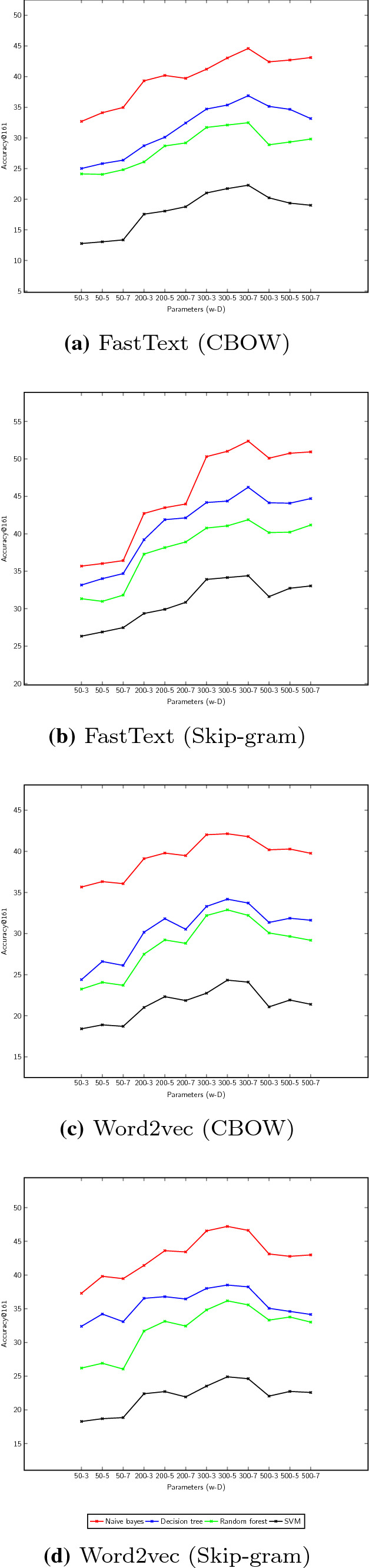
Evaluation of the impact of window size and dimensionality on FastText and Word2vec variants when applied on Covid-large

Experimental settings

Hyper-parameters.

In Table 1, we describe the parameter settings that we use to build the three-word embedding models. We also detail used parameters to build the Bi-LSTM in Table 2.

Table 1.

Word embedding parameters

Parameter	Word2vec	FastText	Char2vec
Vector dimension	50,200,300,500	50,200,300,500	50,200,300,500
Learning rate	0.025	0.025	0.025
Window size	3, 5, 7	3, 5, 7	3 ,5, 7
Minimum count of words	5	5	5
Epoch	5	5	5
Negative sample	5	5	5
Number of threads	12	12	12
Length of n-grams	–	3	–
LSTM dimension	–	–	256
Number of buckets	–	2.000.000	–

Table 2.

Bi-LSTM network parameters

Parameter	Value
Vector dimension	100
Bi-LSTM layers	2
Bi-LSTM hidden units	2*200
Learning rate	0.2
Dropout	20%
Dropword	0%
Optimizer	Stochastic gradient descent
Initialization of LSTMs	Random uniform [−1; 1]
Training epochs	100.000 iterations
Training batch	Size 100

Data

To the best of our knowledge, this is the first work that approaches the geolocation problem on a set of geotagged tweets that reports on Covid-19. In order to study English variations, we collect shared tweets from the UK and the USA via the twitter4j-stream API over the last two weeks of March 2021. We make the resulting corpus available to the research community through the following link4. Only English tweets that are tagged with longitude/latitude coordinates and with mentioned users’ location are retained and merged into a single corpus. Each tweet must contain at least one of our predefined list of keywords (covid; covid-19; corona; coronavirus; quarantine; Wuhan; epidemic; pandemic; mask; distancing; respiratory; isolation; infection; sars; asymptomatic; vaccination; UK; variant). Similarly to (Eisenstein et al., 2010), a gold location is assigned for a set of tweets published by the same user. We exclude users who follow more than 1000 other users and have more than 1000 followers such as celebrities whose may have a large social graph connectivity. In addition, we keep only users with a minimum of four shared tweets. Our collection process ends up with Covid-large, a corpus that contains 5.126.078 geotagged tweets sent by 393.257 unique users from the UK and the USA. In order to properly evaluate DeepGeoloc performance on smaller corpora, we refer to Covid-medium and Covid-small that are derived corpora from Covid-large. Covid-medium contains 2.414.236 geotagged tweets that are randomly selected and shared by 141.812 unique users. As for Covid-small, it is composed of 1.122.089 geotagged tweets sent by 94.622 unique users.

For these two corpora, we adopt the same re-partition of data. For more details, randomly chosen 80% of twitterers are used for the training and the remaining 20% for the evaluation. Note that our framework is the first to resolve both tweet and twitterer geolocation problems. This is realized by associating an index to each tweet in addition to its corresponding twitterer identifier.

Evaluation metrics

We use the accuracy metric to measure the geolocation performance of our sub-models:

Accuracy = (true positive + true negative)/number of performed tests

where:

• True positive: The model correctly predicts the region of the tweet in question;

• True negative: The model correctly predicts the region to which the tweet does not belong.

We also use a second measure that is denoted by Accuracy @161 (Cheng et al. (2010)). This latter is proposed to improve the results of geolocation by increasing the possible predictions within a radius of 161km.

Experimental results and analysis

Evaluation of the word embedding models

Similarly to (Lai et al. 2016), we suppose that a good word embedding can be generated by allocating attention to three components: the model, the training parameters and the corpus. We study the impact of these latter in the next parts.

Impact of models

As described in (Bojanowski et al. 2017), we train FastText with a size of n-grams equal to 3. Through Fig. 3a and b, we notice that this model achieves the best geolocation results when its generated vector representations are used as inputs to train the naive Bayes classifier. Less effective results are observed with random forest and decision tree. As for SVM, training this classifier on FastText, Word2vec or Char2vec vectors does not guarantee good results. This may be due to its linear nature which makes it less suitable when multiple classes (states) are defined.

From Fig. 3b and d, we find that with all classifiers, the Skip-gram variants perform better than CBOW. This observation can be explained by the ability of the Skip-gram model to support rare or infrequent words. Due to the absence of writing rules in Twitter, we consider that misspelled words constitute an important portion of infrequent words. The performance of Skip-gram is further improved when it is adopted by FastText which in turn supports misspelled words and OOVs. As results, linguistic features can be better captured even from short and noisy texts like tweets and may serve to resolve the Coronavirus tracking task. This assumption needs to be validated through the application of another model that is devoid of the treatment of such words which is the case of Word2vec. For the Word2vec model, evaluating its performance by training the nonlinear classifier naive Bayes produces the best results similarly to FastText. While the latter achieves a maximum accuracy rate equal to 52.38%, the former achieves 47.21% when the Skip-gram variant is applied. The difference between these results can be explained by the fact that Word2vec treats words as non-decomposable units. In other terms, it assigns different vector representations to misspelled and correct variants of the same word. A deeper interpretation of our results demonstrates that these representations are distant enough that they make the contribution of misspelled words in the geolocation task less important. Compared to Word2vec, a 2.54 % increase in terms of geolocation accuracy is observed when applying the Char2vec model and training naive Bayes with its vectors. Since Char2Vec uses Word2vec as a lookup table, it should generate better results as it supports the Skip-gram variant. However, the results obtained remain lower than those of FastText which can be explained by two facts: (i) the adoption of Word2vec limits the performance of Char2vec given the problems identified above (ii) the Char2vec strategy, which is based on the fragmentation of words, is less efficient when applied on misspelled words.

In conclusion, we think that treating words as bags of n-grams and applying the Skip-gram variant enables better encoding of linguistic features from tweets. Among these features, we need to perform other experiments to determine which combination has higher spatial indications to track Coronavirus efficiently.

Impact of the training parameters on word embedding models

We consider that the window size w and the dimension D are the most determinant parameters to adjust the quality of word embeddings. Through Fig. 3, we demonstrate the impact of potential values of w and D in the geolocation task.

Impact of the window size For FastText, the more w increases, the better the geolocation results of tweets are. This shows that semantic features that are encoded by this model are more effective for our activity than syntactic ones. As described in Sect. 4.1.1, supporting subword information such as characters is not allowed by Word2vec. Consequently, the contribution of misspelled words in the geolocation of Coronavirus related tweets is less important. Similar to FastText, alterations of w have certain effects on Word2vec. The most optimal value of this parameter is equal to 5. This means that Word2vec cannot capture sufficient semantic aspects with a smaller window. This finding is consistent with the limits outlined above. Otherwise, a limited context is not sufficient to capture the semantic features in a tweet, especially when it contains OOVs or misspelled words.

For char2vec, the single parameter to evaluate is w. From Fig. 4, we see that a contextual window of a size equal to 5 allows having the best geolocation results. The little increase of accuracy rates compared to those of Word2vec demonstrates that morphological features are effective for the geolocation task. However, this efficiency is still limited when inaccurate morphological segmentation is carried out due to the presence of misspelled words.

Fig. 4.

Evaluation of the impact of window size on Char2vec

Impact of the dimensionality The determination of optimal vector sizes depends on the task to be performed (Melamud et al. 2016). So, we have to investigate the impact of this parameter when carrying out the geolocation task on Coronavirus data. In the case of FastText, vectors of size 300 provide the best results for tweet geolocation. Beyond this value, the performance of this model decreases. We can consider that w=300 is the marginal size for the geolocation task. Such value is big enough to encode semantic information. For word2vec, we observe a fall in the results beyond the same value. Therefore, this model cannot keep its performance for larger dimensions. For more details, larger vectors are not able to capture semantic aspects as the distance between every two words becomes wider. This limit is further accentuated by considering the nature of tweets.

Based on all of these experiments, we find that the FastText model is the most suitable word embedding model for processing already geolocated tweets. In particular, it provides the best geolocation results for these short texts.

Impact of the corpus

Like models and training parameters, the corpus may impact the quality of word embeddings. We pursue our experiments by application of the Skip-gram variant of FastText with w=7 and D= 300, respectively, on Covid-large, Covid-medium and Covid small.

Impact of tweet concatenation By studying (Eisenstein et al. 2010; Roller et al. 2012; Wing and Baldridge 2014), we find that they proceed all to the concatenation of tweets of a given user into a single document before applying their geolocation methods. Evaluating the impact of this operation turns out to be interesting, in particular that our geolocation strategy is initially designed for the geolocation of individual tweets. Two scenarios arise at this level:

• FastText performs better on concatenated tweets. For each twitterer, all tweets are treated as a single vector representation. A single location is estimated as that of the class containing more similar tweets.

• FastText performs better on individual tweets. The location of each tweet is estimated separately. The argmax function is finally applied to determine the location with the higher probability.

Obtained results from the evaluation of these scenarios are described in Table 3. Even with the diversity of tweets’ contents that describe the wide impact of Coronavirus on personal assessment, individual and collective lives, our geolocation strategy works better on concatenated tweets than on individual ones similarly to the other three reference works. Therefore, the FastText model remains able to support the multiplicity of topical relationships for the Coronavirus case. But, this ability has to be tested on a larger number of concatenated tweets per user which corresponds to one of our future perspectives.

Table 3.

Impact of the concatenation of tweets in Covid-large on the performance of FastText

Model	Acc.	Acc.@161
FastText (with concatenation)	39.28	50.49
FastText (without concatenation)	37.41	48.05

As shown in Fig. 3b, FastText achieves 52.38% accuracy@161 by processing a single tweet. This rate is expected to increase when geolocating a given user after proceeding to the concatenation of his tweets. Surprisingly, it decrements in our case and attends 50.49% only. We think that these results can be explained by wrong predictions due to similar writing styles in nearby regions. In addition, manual evaluation of a subset of tweets allowed us to note the presence of a considerable number of “retweets.” The decrease in the accuracy rate of our results shows that the majority of retweets are shared by users close to those who originally wrote them. This brings us back to the idea that the spread of topics on social networks can limit the performance of purely statistical geolocation methods.

Impact of corpus’ particularities From Table 4, we notice a large difference between the obtained results by application of FastText, respectively, on Covid large, Covid-medium and COVID-small. For the latter, we find that the performance of FastText is the smallest, which implies that captured semantic features having spatial indications are less effective.

Table 4.

Impact of corpus’ particularities on the performance of FastText

Corpora
Model	Covid-large		Covid-medium		Covid-small
	Acc.	Acc.@161	Acc.	Acc.@161	Acc.	Acc.@161
FastText	39.28	50.49	36.79	43.06	27.21	35.19

The evaluation of FastText on Covid-medium shows more competitive results. Our accuracy rates reach their maximum when dealing with contained tweets in Covid-large. Therefore, we find that the volume of the corpus has more impact than the multiple topical relationships themselves. This finding demonstrates the ability of FastText as a model created by Facebook to support the multiplicity of such relations on social networks. For the Coronavirus tracking task, this model better learns to differentiate between writing styles by capturing more semantic information from bigger amounts of training data. This ability is still conditioned as explained above, by the amount of data contained in a single entry. Compared to (Eisenstein et al. 2010; Roller et al. 2012; Wing and Baldridge 2014; Rahimi et al. 2017), our geolocation results are modest. This motivates us to investigate the limits of FastText and to make additional improvements to our geolocation strategy. Note that in the rest of our experiments, we tried to reproduce the proposed methods in the reference works in order to test them on our Coronavirus corpora and then to properly evaluate the performance of our model.

Contribution of the Mimick model in the geolocation task

We try to improve our geolocation strategy by feeding FastText’s embeddings in the Mimick model. When applying FastText, the recognition of misspelled words and OOVs is conditioned by the similarity of their n-grams with those of words in the training corpus. Being a character-based embedding model, Mimick can improve the performance of FastText by incorporating more orthographic features.

The results of combining the representations of these two models for the geolocation of tweets and users are described in Table 5 and Table 6, respectively. We find that accuracy rates of user geolocation in Table 6 increase compared to those in Table 4. We can interpret this improvement by the contribution of misspelled words and OOVs that are recognized by Mimick. The difference between the accuracy rates in Table 5 and Table 6 shows that the number of retweets and of shared tweets from nearby regions remains significant. We can also explain this by the ability of FastText + Mimick to keep in some measure, its sensitivity to the spatial distribution of similar linguistic features.

Table 5.

Detailed results of our sub-models for the tweet geolocation task

Corpora
Model	Covid-large		Covid-medium		Covid-small
	Acc.	Acc.@161	Acc.	Acc.@161	Acc.	Acc.@161
FastText+Mimick	45.38	57.11	39.25	48.41	30.21	41.07
FastText+Mimick+Des.Model	48.18	58.63	43.50	53.39	38.12	46.29
FastText+ TF-IDF	41.12	48.51	32.43	44.08	29.47	39.77
FastText+Mimick+Att. Model	53.89	64.16	45.87	54.11	35.69	45.58
DeepGeoloc	58.31	66.09	47.61	56.72	41.06	48.35

Table 6.

Results of our model and baselines for the user geolocation task

Corpora
Model	Covid-large		Covid-medium		Covid-small
	Acc.	Acc.@161	Acc.	Acc.@161	Acc.	Acc.@161
Eisenstein et al. (2010)	39.82	51.34	34.19	46.61	27.18	38.75
Wing and Baldridge (2011) (Uniform)	37.66	47.59	30.46	38.70	23.33	31.49
Wing and Baldridge (2011) (K-d tree)	36.14	46.12	28.40	37.93	23.96	29.40
Roller et al. (2012)	30.68	43.22	27.75	37.11	18.47	28.16
Rahimi et al. (2017) (MLP+ K-d tree)	48.90	57.19	41.39	48.03	31.71	39.21
Rahimi et al. (2017) (MLP+ K-means)	49.28	59.81	42.25	49.82	31.88	40.35
FastText+Mimick	43.14	54.93	35.60	45.89	24.37	36.21
FastText+Mimick+Des.model	46.20	56.61	38.25	47.19	30.64	39.84
FastText+ TF-IDF	37.39	45.04	29.72	40.35	22.47	34.69
FastText+Mimick+Att. model	51.13	62.89	41.97	48.62	29.08	37.17
DeepGeoloc	56.20	64.59	42.94	51.23	32.76	42.09

Evaluation of the WSD model

By applying the WSD model, we note a considerable increase in the accuracy rates of our framework, in particular for single tweets in the Covid-small and the Covid-medium corpora (Table 5). A smaller increase is observed for Covid-large as well. We think that the volume of training data is advantageous for: (i) learning more semantic relationships and (ii) differentiating the various usages of words according to their contexts. In our case, we estimate that the WSD model can be more effective on large corpora that contain other topics’ descriptions in addition to those related to Covid-19. Otherwise, the WSD may reach a state of stagnation at a certain level given the similarity of contained contextual information in our corpora. We also notice that our model becomes more sensitive to words that have less significant spatial indications. Diversely, we show that our geolocation accuracy can be enhanced by considering even nonlocal words and delimiting their geosemantic distribution.

Evaluation of the attention model

Determining the most important words in a tweet by learning long-term dependencies is the subject of a final improvement in our geolocation strategy. To be comparable with prior works that apply TF-IDF for identifying local words, we evaluate the contribution of this method on our geolocation results. For more details, we start by applying TF-IDF on the whole corpus similarly to (Lee et al. 2014). After training FastText, the vector representation of each word will be redefined by multiplying it by the calculated weight. Note that we omit the evaluation of TF-IDF when the Mimick model is applied. In fact, the former assigns null values to non-observed words in the training data. Consequently, the combination of Mimick and TF-IDF will not be effective for the geolocation of new tweets that contain OOVs. Taking into account the differences in corpora sizes, described results in Table 5 show that weighting of the words using TF-IDF performs slightly better on Covid-small than on Covid-medium and Covid-large. For these two latter, this low contribution can be explained as follows: The TF-IDF model determines the importance of a word according to its frequency in a given document. Then, its performance decreases as it is not able to establish a correspondence between a local word and its misspelled variants. This decrease is more marked when dealing with a larger corpus and where the word frequency might become wider. Trained on the vector representations that are produced by FastText and Mimick, our attention model achieves better results for the two geolocation tasks. In this regard, we think that the implication of words’ orders in addition to their occurrences makes the redefinition of their importance in a given tweet more accurate. In convergence with our work, sensitivity towards local words decreases when linguistic features encoded by their contexts refer to other locations. Thus, we better distinguish the various uses of local words from bigger corpora notably after a WSD process as illustrated in Table 5 and Table 6. We also find from these tables that differences in the final results between the two geolocation activities decrease proportionally to the sizes of corpora. This can be interpreted by the role of sequential modeling for a better capturing of linguistic features on the one hand and differentiating spatial indications of words from their surrounding contexts on the other hand.

Our results are competitive compared to Roller et al. (2012) and Wing and Baldridge (2011) and close to those of Eisenstein et al. (2010) for the Covid-small corpus. In fact, Eisentein’s work is basically conceived to identify topics and their regional variations. It performs better on this corpus which reflects its performance to determine regional variations of topics. However, this work loses its effectiveness gradually when applied on bigger Corpora like Covid-medium and Covid-large. A reciprocal impact of the corpora size on the geolocation approach is observed with the work of (Rahimi et al. 2017) which realises close results to ours when trained on Covid-small. For more details, the geolocation accuracy increases when applied on larger corpora. We explain this by the contribution of the corpus size to capture deeper relationships between words. Compared to (Rahimi et al. 2017), our neural networks-based approach keeps its efficiency which reminds us of the role of extracted linguistic features specially when adopting a sequential treatment of texts to geolocate tweets. At last, we think that we have to evaluate the applicability of these works on new datasets to justify our empirical choices and to finally decide which geolocation methods are more effective.

Evaluation of DeepGeoloc’s scalability

As indicated in Table 4, our geolocation strategy performs better proportionally to the corpus size. In this context, the distributed architecture of DeepGeoloc can be advantageous to handle large volume of data and implicitly to enhance our geolocation results by treating more linguistic features during the training phase. Thus, evaluating its scalability seems to be interesting in order to validate our technical choices. To do this, we perform some experiments in a cluster of machines that operate with Linux Ubuntu 18.04. Each single machine is equipped with 500 of local storage, 8GB of main memory and 4 CPU. We also use Apache Spark version 2.4.7, Apache kafka version 2.7.0 and Apache Hadoop version 2.9.2 for our experimental architecture. Being an in-memory processing-based framework, input-output concerns are not considered when using Spark and consequently no latency problem is posed. This enables us to conduct our experiments more accurately regarding the impact of the data volume on the processing time. Note that we perform our experiments on subsets of contained tweets in Covid-large with varied sizes by keeping the same data re-partition as described in Sect. 6.2. From Fig. 5, we obviously notice that the average processing time increases proportionally with the volume of data. For more details, we find that Spark becomes slower when we use larger data.

Fig. 5.

Impact of the machines number and data size on the average processing time

In addition to the data volume, we rate the horizontal scalability of DeepGeoloc’s distributed architecture based on the number of machines. Otherwise, we try to measure the impact of machines number on the average processing time. To do this, we create a Spark cluster and vary the number of machines from 3 to 8. Performed on Covid-large, the results presented in Fig. 5 show that the processing time depends on the cluster’s size: when the number of participating machine increases, data processing becomes faster. In our case, 8 machines allow better processing of our data in a shorter time. Using 7 machines, similar results are achieved so that we can limit our experimental architecture to this cluster size for a lower usage of computational resources. Finally, our experiments demonstrate that the distributed architecture of DeepGeoloc is scalable enough to process huge amounts of data in acceptable deadlines. In fact, taking into account the training parameters (D=300 and w=7) of our embeddings for the Coronavirus tracking and given that no Spark crashes occur during the experiments, we think that the average processing time could be acceptable especially when there is no need to reconstruct our models to handle new data as demonstrated later.

Evaluation of DeepGeoloc’s applicability on new data

We aim to evaluate DeepGeoloc’s applicability when processing new datasets. Our assessment is based on four main factors: (i) applicability of the model on new topics, (ii) applicability of the model on new tweets shared by different users from those in the training data, (iii) applicability of the model on new tweets from different periods of time and (iv) applicability of the model on the same English variant which makes the differentiation of regional variations more defiant. To conduct this assessment, we are collecting two corpora containing 527.542 and 988.135 geotagged tweets, respectively. As depicted in Fig. 6, gathered tweets in the first corpus are divided equally over 4 weeks time (week 1, week 2, week 3 and week 4). Those contained in the second one are more recent and spread equally over the last week of March and the first week of April 2021 (week 5 and week 6). For both corpora, tweets are shared from five American states: Texas, New York, California, Florida and Kansas. We choose non-neighboring states as our goal is to measure the applicability of the model on new datasets rather than its performance against similar linguistic features. In regard to covered ahead topics, the first corpus describes the 2020 presidential elections in the USA where selected keywords to collect tweets are the following: Trump, Biden, elections, Democrate, Republican, policy, campaign and vote. The second corpus deals with the impact of Coronavirus on the political orientation and decisions in those states where associated keywords are: Biden, senate, fund, legislative, Democrate, Republican and policy. Note that each tweet must contain at least: (i) one of our preselected keywords which are related to Coronavirus and (ii) one word that describes the current policy-related topics. Note also that the reason behind choosing such topics is to demonstrate the impact of political polarization on shared tweets about Coronavirus across the USA as discussed in Jiang et al. (2020). In order to investigate this impact, we find that filtering tweets by checking the presence of at least one word describing these topics in addition to Coronavirus keywords is feasible.

Fig. 6.

Applicability of DeepGeoloc and baselines on new tweets

We point out that we filter contained tweets in Covid-large and we keep only those shared from the USA as training sets. Applied on the two new corpora, the higher accuracy@161 rate (38.63%) is reached by DeepGeoloc. This result validates our choices of the word embedding models and Bi-LSTMs for an applicable geolocation strategy on new datasets. Technically, we demonstrate the ability of FastText and Mimick to construct vectors for new words from n-gram vectors and characters that constitute those words. Then, we believe that a sequential extraction of linguistic features using such neural networks can reduce possible failures of the geolocation models when processing new data even written in a single English variant. Less competitive results are generated when applying Rahimi et al. (2017) models. Taking into consideration the sizes of the new American datasets, the results obtained by applying the approach of Eisenstein et al. (2010) are unexpectedly insufficient. Hence, similarly to the rest of the works, these results prove that a statistical approach is less adequate to handle the diversity of writing styles despite the limited number of treated topics. Finally, no significant impacts are observed for all works regarding the temporal aspect. This finding is validated at a month scale and may be different for longer data collection periods (years) which necessitates to be verified in our future works.

Conclusion and future work

In this paper, we approach the geolocation of both tweets and twitterers from a new perspective. We evaluate our model on a noticeable topic which is the propagation of the Coronavirus. For this aim, we deal with linguistic features in two variants of English language instead of relying on purely statistical methods to estimate the geographic distribution of words. We demonstrate that contextual information is effective to support misspelled variants and OOVs which prove in turn to have spatial indications. By testing a set of word embedding models, we find that semantic features are the most prominent information for the Coronavirus tracking task in addition to orthographic ones. We demonstrate also that sequential treatment of words by adopting a Bidirectional long short-term memory (Bi-LSTM) architecture increases the geolocation accuracy. On the whole, our neural network-based approach shows that it is scalable enough to handle huge amounts of data using some Apache frameworks. It also demonstrates its applicability on new and noisy textual components describing new topics attached to the Coronavirus even at a state level. In the future, we plan to evaluate the performance of DeepGeoloc when applied to differentiate variants of the same language at a more granular geographic scale. From a technical perspective, we plan to study the impact of additional parameters like the data collection time, the length of character n-grams and the number of tweets per user. We also think that it will be interesting to evaluate generated results in near-real time. This is particularly interesting where the processing time is crucial to plan emergency interventions and to delimit infected geographic areas by Coronavirus. To do this, we think that boosting the DeepGeoloc’s distributed architecture with quasi-recurrent neural networks may be an effective solution to geolocate tweets in shorter time. Finally, we seek to evaluate extended versions of RNNs that support spatial and temporal contexts to keep tracking of new actualities and personal assessments declared in tweets in relation to the Coronavirus pandemic.

Declarations

Conflict of interest

The authors declare that the research was conducted in the absence of any commercial or financial relationships that could be construed as a potential conflict of interest.

References

- Ahmouda A, Hochmair HH, Cvetojevic S. Analyzing the effect of earthquakes on openstreetmap contribution patterns and tweeting activities. Geo-spatial Inf Sci. 2018;21(3):195–212. doi: 10.1080/10095020.2018.1498666. [DOI] [Google Scholar]
- Ao J, Zhang P, Cao Y (2014) Estimating the locations of emergency events from twitter streams. In: 2nd International Conference on Information Technology and Quantitative Management (ITQM), pp 731–739
- Arora M, Kansal V. Character level embedding with deep convolutional neural network for text normalization of unstructured data for twitter sentiment analysis. Soc Netw Anal Min. 2019;9(1):12. doi: 10.1007/s13278-019-0557-y. [DOI] [Google Scholar]
- Backstrom L, Kleinberg J, Kumar R, Novak J (2008) Spatial variation in search engine queries. In: Proceedings of the 17th international conference on World Wide Web (WWW), pp 357–366
- Ballatore A, Wilson DC, Bertolotto M. Computing the semantic similarity of geographic terms using volunteered lexical definitions. Int J Geogr Inf Sci. 2013;27(10):2099–2118. doi: 10.1080/13658816.2013.790548. [DOI] [Google Scholar]
- Beldad A, Kusumadewi MC. Here’s my location, for your information: the impact of trust, benefits, and social influence on location sharing application use among indonesian university students. Comput Hum Behav. 2015;49:102–110. doi: 10.1016/j.chb.2015.02.047. [DOI] [Google Scholar]
- Bhoi A, Pujari SP, Balabantaray RC. A deep learning-based social media text analysis framework for disaster resource management. Soc Netw Anal Min. 2020;10(1):1–14. doi: 10.1007/s13278-020-00692-1. [DOI] [Google Scholar]
- Bojanowski P, Grave E, Joulin A, Mikolov T. Enriching word vectors with subword information. Transac Assoc Comput Linguistics. 2017;5:135–146. doi: 10.1162/tacl_a_00051. [DOI] [Google Scholar]
- Cao K, Rei M (2016) A joint model for word embedding and word morphology. In: Proceedings of the 1st Workshop on Representation Learning for NLP (RepL4NLP), ACL, pp 18–26
- Chang Hw, Lee D, Eltaher M, Lee J (2012) @ phillies tweeting from philly? predicting twitter user locations with spatial word usage. In: 2012 IEEE/ACM International Conference on Advances in Social Networks Analysis and Mining (ASONAM), IEEE, pp 111–118
- Cheng Z, Caverlee J, Lee K (2010) You are where you tweet: a content-based approach to geo-locating twitter users. In: Proceedings of the 19th ACM International Conference on Information and knowledge management (CIKM), pp 759–768
- Cui R, Agrawal G, Ramnath R. Tweets can tell: activity recognition using hybrid gated recurrent neural networks. Soc Netw Anal Min. 2020;10(1):1–15. doi: 10.1007/s13278-020-0628-0. [DOI] [Google Scholar]
- De Albuquerque JP, Herfort B, Brenning A, Zipf A. A geographic approach for combining social media and authoritative data towards identifying useful information for disaster management. Int J Geogr Inf Sci. 2015;29(4):667–689. doi: 10.1080/13658816.2014.996567. [DOI] [Google Scholar]
- Do TH, Nguyen DM, Tsiligianni E, Cornelis B, Deligiannis N (2018) Twitter user geolocation using deep multiview learning. 2018 IEEE International Conference on Acoustics. Speech and Signal Processing (ICASSP), IEEE, pp 6304–6308
- Ebrahimi M, ShafieiBavani E, Wong R, Chen F (2018) A unified neural network model for geolocating twitter users. In: Proceedings of the 22nd Conference on Computational Natural Language Learning (CONLL), pp 42–53
- Eisenstein J, O’Connor B, Smith NA, Xing EP (2010) A latent variable model for geographic lexical variation. In: Proceedings of the 2010 Conference on Empirical Methods in Natural Language Processing (EMNLP), ACL, pp 1277–1287
- Elaraby M, Abdul-Mageed M (2018) Deep models for arabic dialect identification on benchmarked data. In: Proceedings of the Fifth Workshop on NLP for Similar Languages, Varieties and Dialects (VarDial 2018), pp 263–274
- Guellil I, Azouaou F, Chiclana F. Arautosenti: automatic annotation and new tendencies for sentiment classification of arabic messages. Soc Netw Anal Min. 2020;10(1):1–20. doi: 10.1007/s13278-020-00688-x. [DOI] [Google Scholar]
- Han B, Cook P, Baldwin T (2012) Geolocation prediction in social media data by finding location indicative words. In: Proceedings of the International Conference on Computational Linguistics (COLING), pp 1045–1062
- Hawelka B, Sitko I, Beinat E, Sobolevsky S, Kazakopoulos P, Ratti C. Geo-located twitter as proxy for global mobility patterns. Cartogr Geogr Inf Sci. 2014;41(3):260–271. doi: 10.1080/15230406.2014.890072. [DOI] [PMC free article] [PubMed] [Google Scholar]
- Hecht B, Hong L, Suh B, Chi EH (2011) Tweets from justin bieber’s heart: the dynamics of the location field in user profiles. In: Proceedings of the SIGCHI Conference on Human Factors in Computing Systems, pp 237–246
- Hochreiter S. The vanishing gradient problem during learning recurrent neural nets and problem solutions. Internat J Uncertain Fuzziness Knowledge-Based Syst. 1998;6(02):107–116. doi: 10.1142/S0218488598000094. [DOI] [Google Scholar]
- Hochreiter S, Schmidhuber J (1997) Lstm can solve hard long time lag problems. In: Advances in Neural Information Processing Systems, pp 473–479
- Hu Y, Ye X, Shaw SL. Extracting and analyzing semantic relatedness between cities using news articles. Int J Geogr Inf Sci. 2017;31(12):2427–2451. doi: 10.1080/13658816.2017.1367797. [DOI] [Google Scholar]
- Jiang B, Ren Z. Geographic space as a living structure for predicting human activities using big data. Int J Geogr Inf Sci. 2019;33(4):764–779. doi: 10.1080/13658816.2018.1427754. [DOI] [Google Scholar]
- Jiang J, Chen E, Yan S, Lerman K, Ferrara E. Political polarization drives online conversations about covid-19 in the united states. Human Behav Emerging Technol. 2020;2(3):200–211. doi: 10.1002/hbe2.202. [DOI] [PMC free article] [PubMed] [Google Scholar]
- Kejriwal M, Zhou P. On detecting urgency in short crisis messages using minimal supervision and transfer learning. Soc Netw Anal Min. 2020;10(1):1–12. doi: 10.1007/s13278-020-00670-7. [DOI] [PMC free article] [PubMed] [Google Scholar]
- Lai S, Liu K, He S, Zhao J. How to generate a good word embedding. IEEE Intell Syst. 2016;31(6):5–14. doi: 10.1109/MIS.2016.45. [DOI] [Google Scholar]
- Larson JM, Nagler J, Ronen J, Tucker JA. Social networks and protest participation: Evidence from 130 million twitter users. Am J Political Sci. 2019;63(3):690–705. doi: 10.1111/ajps.12436. [DOI] [Google Scholar]
- Lau JH, Chi L, Tran KN, Cohn T (2017) End-to-end network for twitter geolocation prediction and hashing. In: Proceedings of the 8th International Joint Conference on Natural Language Processing (ICNLP) (Volume 1: Long Papers), Asian Federation of Natural Language Processing, pp 744–753
- Lee K, Ganti RK, Srivatsa M, Liu L (2014) When twitter meets foursquare: tweet location prediction using foursquare. In: Proceedings of the 11th international conference on mobile and ubiquitous systems: Computing, networking and services, ICST, pp 198–207
- Levy O, Goldberg Y (2014) Dependency-based word embeddings. In: Proceedings of the 52nd Annual Meeting of the Association for Computational Linguistics (Volume 2: Short Papers), pp 302–308
- Lingad J, Karimi S, Yin J (2013) Location extraction from disaster-related microblogs. In: Proceedings of the 22nd international conference on WWW, pp 1017–1020
- Ma D, Osaragi T, Oki T, Jiang B. Exploring the heterogeneity of human urban movements using geo-tagged tweets. Int J Geograph Inf Sci. 2020;1:1–22. [Google Scholar]
- Martinez LS, Hughes S, Walsh-Buhi ER, Tsou MH. okay, we get it you vape: an analysis of geocoded content, context, and sentiment regarding e-cigarettes on twitter. J Health Commun. 2018;23(6):550–562. doi: 10.1080/10810730.2018.1493057. [DOI] [PubMed] [Google Scholar]
- Melamud O, McClosky D, Patwardhan S, Bansal M (2016) The role of context types and dimensionality in learning word embeddings. In: 2016 Annual Conference of the North American Chapter of the Association for Computational Linguistics: Human Language Technologies (NAACL-HLT), pp 1030–1040
- Melo F, Martins B (2015) Geocoding textual documents through the usage of hierarchical classifiers. In: Proceedings of the 9th Workshop on Geographic Information Retrieval, pp 1–9
- Mikolov T, Chen K, Corrado G, Dean J (2013a) Efficient estimation of word representations in vector space. In: Proccedings of the 1st International Conference on Learning Representations
- Mikolov T, Sutskever I, Chen K, Corrado GS, Dean J (2013b) Distributed representations of words and phrases and their compositionality. In: Advances in Neural Information Processing Systems, pp 3111–3119
- Miura Y, Taniguchi M, Taniguchi T, Ohkuma T (2016) A simple scalable neural networks based model forgeolocation prediction in twitter. In: Proceedings of the 2nd Workshop on Noisy User-generated Text (WNUT), pp 235–239
- Mohammed A, Kora R. Deep learning approaches for arabic sentiment analysis. Soc Netw Anal Min. 2019;9(1):52. doi: 10.1007/s13278-019-0596-4. [DOI] [Google Scholar]
- Ombabi AH, Ouarda W, Alimi AM. Deep learning cnn-lstm framework for arabic sentiment analysis using textual information shared in social networks. Soc Netw Anal Min. 2020;10(1):1–13. doi: 10.1007/s13278-020-00668-1. [DOI] [Google Scholar]
- Paraskevopoulos P, Palpanas T (2015) Fine-grained geolocalisation of non-geotagged tweets. In: Proceedings of the 2015 IEEE/ACM International Conference on ASONAM, IEEE, pp 105–112
- Pinter Y, Guthrie R, Eisenstein J (2017) Mimicking word embeddings using subword rnns. In: 2017 Conference on EMNLP, pp 102–112
- Priedhorsky R, Culotta A, Del Valle SY (2014) Inferring the origin locations of tweets with quantitative confidence. In: Proceedings of the 17th ACM Conference on Computer Supported Cooperative Work & Social Computing, pp 1523–1536 [DOI] [PMC free article] [PubMed]
- Rahimi A, Cohn T, Baldwin T (2017) A neural model for user geolocation and lexical dialectology. In: Proceedings of the 55th Annual Meeting of the ACL (Volume 2: Short Papers), ACL, pp 209–216
- Roller S, Speriosu M, Rallapalli S, Wing B, Baldridge J (2012) Supervised text-based geolocation using language models on an adaptive grid. In: Proceedings of the 2012 Conference on CoNLL, ACL, pp 1500–1510
- Singh P, Sawhney RS, Kahlon KS. Sentiment analysis of demonetization of 500 & 1000 rupee banknotes by indian government. ICT Express. 2018;4(3):124–129. doi: 10.1016/j.icte.2017.03.001. [DOI] [Google Scholar]
- Sizov S (2010) Geofolk: latent spatial semantics in web 2.0 social media. In: Proceedings of the third ACM International Conference on Web Search and Data Mining (WSDM), pp 281–290
- Tran T, Lee K (2016) Understanding citizen reactions and ebola-related information propagation on social media. In: 2016 IEEE/ACM International Conference on ASONAM, IEEE, pp 106–111
- Tshimula JM, Chikhaoui B, Wang S. A new approach for affinity relationship discovery in online forums. Social Netw Analys Mining. 2020;10(1):40. doi: 10.1007/s13278-020-00644-9. [DOI] [Google Scholar]
- Wang C, Wang J, Xie X, Ma WY (2007) Mining geographic knowledge using location aware topic model. In: Proceedings of the 4th ACM Workshop on Geographical Information Retrieval, pp 65–70
- Wing B, Baldridge J (2014) Hierarchical discriminative classification for text-based geolocation. In: Proceedings of the 2014 Conference on EMNLP, pp 336–348
- Wing BP, Baldridge J (2011) Simple supervised document geolocation with geodesic grids. In: Proceedings of the 49th Annual Meeting of the ACL: Human language technologies (Volume 1), ACL, pp 955–964
- Xu P, Dredze M, Broniatowski DA. The twitter social mobility index: Measuring social distancing practices with geolocated tweets. J Med Internet Res. 2020;22(12):e21499. doi: 10.2196/21499. [DOI] [PMC free article] [PubMed] [Google Scholar]
- Yuan D, Richardson J, Doherty R, Evans C, Altendorf E (2016) Semi-supervised word sense disambiguation with neural models. In: Proceedings of the 26th International Conference on Computational Linguistics: Technical Papers, p 1374-1385
- Yuan S, Wu X, Xiang Y. Incorporating pre-training in long short-term memory networks for tweet classification. Soc Netw Anal Min. 2018;8(1):52. doi: 10.1007/s13278-018-0530-1. [DOI] [Google Scholar]
- Zhang X, Zhang L. Topics extraction in incremental short texts based on lstm. Soc Netw Anal Min. 2020;10(1):1–9. doi: 10.1007/s13278-020-00699-8. [DOI] [Google Scholar]
- Zhao B, Sui DZ. True lies in geospatial big data: detecting location spoofing in social media. Ann GIS. 2017;23(1):1–14. doi: 10.1080/19475683.2017.1280536. [DOI] [Google Scholar]
- Zola P, Cortez P, Carpita M. Twitter user geolocation using web country noun searches. Decis Support Syst. 2019;120:50–59. doi: 10.1016/j.dss.2019.03.006. [DOI] [Google Scholar]