The Importance of Making Assumptions in Bias Analysis

Abstract

Quantitative bias analyses allow researchers to adjust for uncontrolled confounding, given specification of certain bias parameters. When researchers are concerned about unknown confounders, plausible values for these bias parameters will be difficult to specify. Ding and VanderWeele developed bounding factor and E-value approaches that require the user to specify only some of the bias parameters. We describe the mathematical meaning of bounding factors and E-values and the plausibility of these methods in an applied context. We encourage researchers to pay particular attention to the assumption made, when using E-values, that the prevalence of the uncontrolled confounder among the exposed is 100% (or, equivalently, the prevalence of the exposure among those without the confounder is 0%). We contrast methods that attempt to bound biases or effects and alternative approaches such as quantitative bias analysis. We provide an example where failure to make this distinction led to erroneous statements. If the primary concern in an analysis is with known but unmeasured potential confounders, then E-values are not needed and may be misleading. In cases where the concern is with unknown confounders, the E-value assumption of an extreme possible prevalence of the confounder limits its practical utility.

Although epidemiologic data may be affected by many types of bias, uncontrolled confounding is almost always a central concern in observational studies.¹ Methods for quantitative bias analysis have been available since at least the 1950s and allow researchers to adjust effect-measure estimates for uncontrolled confounding.^2–12 Such methods typically require the researcher to specify three parameters: the strength of the association between an uncontrolled confounder and the disease conditional on exposure, the strength of the association between the confounder and the exposure, and the distribution of the confounder given exposure. A researcher interested in adjusting for uncontrolled confounding needs to specify values for each of these three parameters and substitute them into the requisite formula.^13,14 When a researcher can name a potential confounder that was left uncontrolled by the conventional analysis, it may be feasible to provide plausible estimates or prior probability distributions for these bias parameters based on background literature. However, when there is concern about yet unknown or unsuspected confounders, plausible values for these parameters may be difficult to specify based on credible contextual information.

Ding and VanderWeele¹⁵ proposed an approach that attempts to fill this gap.¹⁶ They developed a bounding factor that requires the user to specify only the strength of the confounder–exposure and confounder–disease associations. They show how, given these associations, one can calculate bounds on what the exposure-effect estimate would be. These bounds are attained when the confounder prevalence among the exposed (or equivalently the exposure prevalence among those without the confounder) is at the value that generates maximum bias.

The E-value inverts this approach by asking: If the confounder–exposure and confounder–disease associations are equal, what is the smallest size this association must have for control of the confounder to “explain away” the observed exposure–disease association, given the confounder prevalence among the exposed is at the value that generates maximum bias? That is, the E-value is the smallest confounder association with exposure, and confounder association with disease given exposure, needed for confounding to create the observed exposure–disease association entirely, when no exposure effect truly exists, under an extreme-case scenario in which all exposed people have the confounder.

As with all methods, the proposed bounding factors and E-values are only as valid as their assumptions.^17–20 It is thus crucial that their underlying assumptions are understood correctly, both in their mathematical meaning and their plausibility in an applied context, and that is our focus here. We also delineate the critical distinction between methods (such as the E-value) that attempt to place bounds on possible biases or effects, and alternative approaches (such as quantitative bias analysis) that attempt to directly account for uncontrolled biases via adjustments to point and interval estimates. For further debate on the problems of E-values, see the recent exchange in the International Journal of Epidemiology.^19,21–24

METHODS

Bias and Bounding Factors

Ding and VanderWeele¹⁵ introduce their bounding factor and derive the E-value under a general specification, which does not require an assumption that the confounder is binary. To simplify the exposition, we will derive the necessary results using the approach of Schlesselman⁵, which Ding and VanderWeele¹⁵ also show in their Appendix. We assume the estimation target is the risk ratio for the effect of a binary exposure, E, on a binary outcome, D, and we have observed an unadjusted estimate of this ratio (). We imagine that there is a binary covariate, U, that may confound this estimate, and that multiplies outcome risk by RR_UD, regardless of exposure (that is, there is no multiplicative interaction between U and E). We denote the prevalence of U among the unexposed by p₀, the prevalence of U among the exposed by p₁, and the ratio relating E to U by RR_EU = p₁/p₀.

For simplification, we will ignore random error and assume that RR_EU and RR_UD are both greater than 1 (as Ding and VanderWeele¹⁵ assumed), so the uncontrolled confounding by U is upward. Our assumption that the ratio effect of U, RR_UD, is constant across exposure levels implies that the risk ratio relating exposure to disease is constant across levels of U, which we call the adjusted association, . Under these assumptions, the bias factor ,

(1)

can be written^5,15

(2)

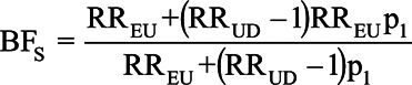
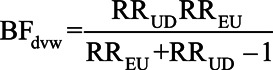
Citing concerns over subjectivity in specifying values to assign to the bias parameters, Ding and VanderWeele¹⁵ noted that the bias factor, BF_s, is monotonically increasing over the range of p₁, so to derive an upper bound on how extreme the bias could be, they assumed the prevalence of the confounder among the exposed is 100% (p₁ = 1). This assumption is equivalent to assuming that the prevalence of the exposure among those without the confounder is 0%. Replacing p₁ with 1 in BF_s produces the bias bounding factor

(3)

When p₁ = 1, RR_EU is well-defined, but there is no one who is exposed and without the confounder; thus, RR_UD would suffer from a positivity violation in the exposed stratum and thus is numerically undefined (in the sense of dividing by zero). Nonetheless, this imposes no constraint on RR_UD in the exposed stratum, and as p₁ approaches 1, RR_UD in the exposed stratum remains constant at the value seen in the unexposed stratum (which remains defined when p₁ = 1). The relations we describe hold mathematically as p₁ approaches 1, and make sense conceptually insofar as the limit shows the effect U had on D among the exposed, which is real even if all the exposed had U (p₁ = 1) and thus all experienced this U effect. Nonetheless, a major point of E-value critiques, including ours, is that this limit can be far from what would be seen as plausible in light of background and data information.

Consider a hypothetical situation in which the RR_UD = RR_EU = 2. As shown in Figure 1, BF_s is less than or equal to BF_dvw at every possible confounder prevalence, which is why Ding and VanderWeele¹⁵ refer to BF_dvw as a sharp bounding factor. The two bias formulas give the same answer only when the prevalence of the confounder in the exposed is 1. The two formulas are maximally different when the prevalence of the confounder among the exposed is 0, since in this case, there can be no upward confounding by U. In this situation, BF_s = 1, while BF_dvw still indicates that the bias is less than or equal to 1.33. These two statements are compatible; however, BF_dvw could mislead if its status as an upper bound is not kept in mind.

FIGURE 1.

Bias factors for the extent of confounding when RR_EU = RR_UD = 2 and RR_obs > 1 over the range of possible values of the prevalence of the confounder in the exposed. Solid line is the Schlesselman bias factor, BF_s, and dashed line is the bounding factor of Ding and VanderWeele,¹⁵ BF_dvw.

The Schlesselman bias factor can be used to adjust an observed RR for uncontrolled confounding; values for RR_UD, RR_EU, and p₁ are first used in equation (2) to estimate BF_s, which is then used in equation (1) to adjust the observed RR

Ding and VanderWeele¹⁵ propose to use BF_dvw in the same way: After specifying values for RR_UD and RR_EU, BF_dvw is calculated from equation (3) and then substituted into equation (1). However, because the Ding and VanderWeele¹⁵ approach assumes a value of p₁ that maximizes the bias factor, the bias-adjusted estimate produced by their approach is only a lower bound on the adjusted estimate and may be substantially lower than the bias-adjusted estimate obtained by the Schlesselman approach.

Example 1

VanderWeele and Ding¹⁶ illustrate their bounding factor in a case–control study examining the association between formula feeding (relative to breastfeeding) and respiratory infections among infants. Victora et al²⁵ found a substantial association (RR = 3.9) between formula use (breastfeeding was the reference category) and respiratory infections; however, they did not ascertain whether women smoked, so were unable to control for this potential confounder. VanderWeele and Ding¹⁶ assumed the association between smoking and respiratory disease was RR_UD = 4 and the association between formula use (vs. breastfeeding) and smoking was RR_EU = 2. Using these values in equation (3), they found BF_dvw = 1.6; that is, the most that smoking could bias the observed effect would be by a factor of 1.6, if specified associations were correct. This result is only an upper bound on the actual bias, however, and equals that bias only if the prevalence of smoking among women in the formula group is 100%—an exceedingly unlikely scenario. If the prevalence among the exposed is under 100%, BF_dvw = 1.60 simply implies that the actual bias due to this uncontrolled confounder is less than 1.60.

We illustrate the difference between BF_dvw and BF_s, which incorporates information on the prevalence of the confounder. To estimate p₁, the prevalence of smoking among Brazilian women who used exclusively formula during this time period, required three sources of information. First, we estimated the overall prevalence of smoking, p_c, from a study by Barros et al³⁰ (their Table 2), which reported p_c = 35.6%. Second, we estimated the prevalence of formula feeding, p_e, as 119/(119 + 281) = 29.8% using data from the control series in Victora et al²⁵ (their Table 1). Third, we assumed RR_EU = 2.0, as in VanderWeele and Ding.¹⁶ From these three assumptions, we calculated p₁ as 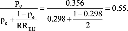Schlesselman’s bias factor under this prevalence is BF_s = 1.45; that is, failure to adjust for smoking would be expected to bias the observed estimate of association by a factor of 1.45.

Both BF_dvw and BF_s can be used in equation (1) to generate a confounding-adjusted effect estimate, yielding values of RR = 2.4 and RR = 2.7, respectively. The value RR = 2.4 obtained by using BF_dvw is a bound on the bias-adjusted RR: it is the smallest possible confounding-adjusted RR that could be obtained using RR_EU = 2 and RR_UD = 4. The value RR = 2.7 is the bias-adjusted RR that would be obtained had we been able to adjust for smoking using the same values for RR_EU and RR_UD along with p₁ = 55% and is, indeed, greater than the Ding and VanderWeele¹⁵ bound of 2.4.

Bounding Factors Versus Probabilistic Bias Analysis

In settings for which there is context-specific concern about a specified but unmeasured potential confounder (as in the example), bounding methods can provide misleading impressions of the magnitude of bias since they are calculated under the most extreme prevalence. Nonetheless, the available contextual information is usually uncertain. Rather than assuming the prevalence p₁ is a specific value, we can produce estimates of bias factors and bias-adjusted effects using probabilistic bias analysis.^{13,14,26–28} Indeed, incorporating parameter uncertainty in the final estimate of effect is a crucial component of probabilistic bias analysis. VanderWeele and colleagues²⁰ have argued that researchers may sometimes want to move past bounds (such as E-values) to probabilistic bias analyses;²⁹ however, it is unclear how often that has happened.²¹

To illustrate, Barros et al³⁰ provide estimates of maternal smoking among pregnant women, overall and by family income, in Brazil, 1982–1984. To specify a prior distribution for p₁, we took p₁ = 0.55 computed above as the mode. We then applied the formula for p₁ in the previous section to data in Barros et al³⁰ Table 2 to specify a possible range for the smoking prevalence among women who formula fed: 31% and 67%. To implement a probabilistic bias analysis, we specified that the prevalence of smoking among women whose infants use formula follows a triangular distribution with a minimum of 0.255, a maximum of 0.717, and a mode of 0.55. These parameters imply that our best guess at the prevalence is 55%, and we have 95% certainty that p₁ is between 31% and 67% and that we are 100% certain it is not less than 25.5% or greater than 71.7%. The mode is the overall smoking prevalence as computed above. The lower 95% limit matches the estimated prevalence of smoking among women who breastfeed in the family income stratum with the lowest overall prevalence of smoking in Barros et al.³⁰ The upper 95% limit is the estimated prevalence in the family income stratum with the highest prevalence of smoking in Barros et al.³⁰

We note that the mode of this distribution is closer to the upper limit than to the upper limit, reflecting the skew of the smoking data in Barros et al,³⁰ where strata with low prevalences of smoking contained fewer women. We drew 10⁶ samples from this distribution and repeatedly inserted the sampled values into equation (2), along with RR_UD = 4 and RR_EU = 2, to produce 10⁶ bias factors. In turn, we used these bias factors to compute 10⁶ confounding-adjusted RRs using equation (1). Accounting for the possible uncertainty in the prevalence of maternal smoking, we estimated a median bias factor of 1.44 (95% simulation limits: 1.32, 1.50).

Figure 2 shows the distribution of the resulting Schlesselman bias factors in relation to the bounding factor BF_dvw from Ding and VanderWeele.¹⁵ The entire distribution of BF_s is substantially lower than BF_dvw, implying that even if we assume substantial uncertainty in prevalence, BF_dvw is a poor estimate of the extent of plausible bias, given the other bias modeling assumptions. Using the sampled values of BF_s in equation (1) to compute a confounding-adjusted RR produced a median RR = 2.72 and 95% simulation limits of 2.60, 2.96. To more directly compare with the result provided by BF_s, we have not included random error in these limits, only uncertainty in the prevalence. Thus, even accounting for our relatively large uncertainty around the actual prevalence of maternal smoking, the lower 95% simulation limit is still substantially larger than the Ding and VanderWeele¹⁵ bound of RR = 2.4. Only if our uncertainty in the prevalence of the confounder placed substantial probability near a prevalence of 100% would the Ding and VanderWeele¹⁵ bound provide a bound compatible with the lower limit from our probabilistic bias analysis.

FIGURE 2.

Distribution of the Schlesselman bias factor BF_s if prevalence is assumed to follow a triangular distribution with minimum = 0.255, maximum = 0.717, and mode = 0.55. Dark vertical line is the limit from the bounding factor, BF_DVW.

Additionally, we incorporated random error into our estimate by randomly resampling from a normal distribution with mean equal to the log of the adjusted RR and variance equal to the variance estimate for the observed (unadjusted) RR. This procedure was repeated for each of the 10⁶ confounding-adjusted RRs and resulted in 95% simulation limits of 1.24, 6.02.

The E-Value

In some settings, researchers might be hesitant to specify values for RR_UD and RR_EU, and here VanderWeele and Ding¹⁶ proposed the E-value, which inverts the bounding factor in (3). First, one assumes that RR_UD = RR_EU and substitutes this quantity into equation (3). Next, if one wants to determine the smallest common value of RR_UD = RR_EU > 1 that could possibly produce enough bias to completely reduce RR_obs to the null, we set BF_dvw = RR_obs. Making these substitutions to equation (3) and solving for E-value gives:

(4)

The E-value is the minimum value for RR_UD = RR_EU > 1 that would make the bounding factor BF_dvw = RR_obs and thus make the lower bound on the adjusted association equal to 1. It is important to note that the E-value function takes RR_obs as an input; unfortunately, using confidence limits in such a bounding function does not produce valid confidence limits for the target risk ratio .³¹ Because the E-value is derived from the bounding factor, BF_dvw, it also assumes the most bias-inducing scenario, that p₁ = 100%. Because confounding is determined by RR_UD and RR_EU in addition to p₁, if we assume p₁ is as deleterious as possible, then to explain away an effect, the shared value of RR_UD and RR_EU does not need to be as large as it would if p₁ were less extreme. Said another way, if the prevalence among the exposed is not 100%, a substantially larger shared value of RR_UD and RR_EU would be required to reduce an observed effect to the null.

The E-value assumes RR_UD and RR_EU are equal, which is another implausible assumption with substantial implications. To see this, note that one of RR_UD and RR_EU could be arbitrarily large and yet U would produce little confounding if the other was nearly 1. For example, using RR_EU = 1.01 and RR_UD = 1,000 in the original Ding and VanderWeele¹⁵ bound, we get BF_dvw = 1.01, or only 1% maximum bias from a variable U that has a stronger effect on disease than anything we see in epidemiology. Using instead RR_EU = 1.10 and RR_UD = 10 we get BF_dvw = 1.09, or only 9% maximum bias (given RR_obs > 1 and assuming RR_adj = 1) from a variable U with an effect comparable to that of smoking on lung cancer. Thus, the E-value can be unlimited in how misleading it becomes, for it assumes an extreme-case scenario: confounder prevalence (p₁) of 100%, and equality of the associations of U with D and E on the risk-ratio scale. Neither assumption has any basis in real examples we are familiar with, and this has led to rejection of the E-value by several authors.^17,18

To see the impact on the E-value of its assumption about p₁, we compute a bias factor using Schlesselman’s formula in (2) assuming that RR_UD = RR_EU and that the observed RR is completely explained away by U, RR_obs = BF_s, but we leave p₁ unspecified. Substituting parameters and solving for the strength of the confounder effects leads to an alternative formula, which we call the generalized E-value and denote by G-value(p₁), which is given by:

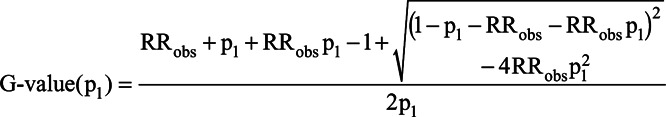Like the E-value, the G-value(p₁) is defined for RR_obs > 1. Reverse coding can be used to accommodate observed effects less than 1. Because we specify a value for p₁, G-value(p₁) is not a bound on the magnitude of the confounder associations; it is the exact size that RR_UD = RR_EU > 1 would need to have to reduce RR_obs to the null, for a given p₁. We note that it is possible to derive a G-value formula under the more general conditions (such as a nonbinary confounder) used in Ding and VanderWeele.¹⁵

Figure 3 shows the relationship between prevalence and G-value(p₁) across a range of prevalences. When p₁ = 100%, the E-value and G-value(p₁) are identical. However, for all other prevalences, the E-value is less than G-value(p₁), illustrating that the E-value has underestimated the required size of the confounder relations needed to nullify the conventional result when p₁ is more realistically specified. As the prevalence diminishes, the discrepancy increases dramatically, with G-value(p₁) increasing over the E-value by orders of magnitude. As seen with BF_dvw, a lower prevalence of the confounder among the exposed implies less confounding, so that to reduce a given value or RR_obs to the null, the magnitude of RR_UD and RR_EU must increase as p₁ decreases. The G-value(p₁) also gives an alternative way of conceiving of the E-value: by setting p₁ = 100%, we minimize the value of RR_EU = RR_UD > 1 that yields a confounding bias equal to RR_obs.

FIGURE 3.

G-value(p₁) for the strength required for equal confounder-exposure and confounder-disease associations RR_EU = RR_UD to reduce an observed RR = 2 to the null. The E-value of Ding and VanderWeele¹⁵ is obtained at G-value(1) = 3.41.

Example 2

Trinquart et al used E-values to estimate the robustness of effects that were published in the nutritional epidemiology and air pollution epidemiology literature.^32–34 The authors abstracted estimates from 100 air pollution studies and 100 nutrition studies that found statistically significant estimates. The focus on statistically significant estimates by Trinquart et al³³ was because “P values drive the nature of published estimates in [these] literature[s].” We note that focusing only on statistically significance is a source of publication bias that results in overestimation when RR > 1 (and underestimation when RR < 1) and that aggregating heterogenous studies that have different health outcomes makes it difficult to draw conclusions.³⁵

Hamra³² raised further criticisms of Trinquart et al.³³ Our focus here is solely on the latter authors’ use of E-values. In the nutritional epidemiology literature, they estimate a median effect estimate across studies of RR = 1.33 and in the air pollution literature, they found a median effect estimate of RR = 1.16, with E-values of 2.00 and 1.59, respectively. The authors state, with regard to the result for the nutrition literature, that it would take “…a relative effect of 2.00 […] to turn the estimate into a null estimate.” This assertion will only be true if the prevalence of the uncontrolled confounder among the exposed is 100% and the prevalence of the exposure is zero in the reference level of the confounder; if the prevalence of the uncontrolled confounder is less, RR_UD = RR_EU = 2.0 will reduce the observed effect, but not all the way to the null.

Trinquart et al³³ never identify any uncontrolled confounder likely to be operating across these literatures. If the concern in these literatures is with confounders that have a prevalence far lower than 100%, as we suspect it is, their inference could change dramatically. For example, if the shared confounder in the nutrition literature had a prevalence among the exposed of p₁ = 10%, RR_UD = RR_EU = 5.4 would be required to reduce the observed association RR_obs = 1.33 to the null (Table). These results would make the existing literature appear more robust to uncontrolled confounding than Trinquart et al³³ implied based on E-values.

TABLE.

The Magnitude of RR_EU = RR_UD Required to Reduce the Observed Air Pollution and Nutritional Associations to the Null, G-Value(p₁), by Prevalence of the Uncontrolled Confounder Among the Exposed

True Prevalence Among the Exposed	Air Pollution Epidemiology (Observed association = 1.16)		Nutritional Epidemiology (Observed Association = 1.33)
	G-Value(p1)	Implied Prevalence Among the Unexposed [p1/G-Value(p1)]	G-Value(p1)	Implied Prevalence Among the Unexposed [p1/G-Value(p1)]
0.1	3.4	0.03	5.4	0.02
0.2	2.5	0.08	3.6	0.06
0.3	2.2	0.14	3.0	0.10
0.4	2.0	0.20	2.7	0.15
0.5	1.9	0.27	2.4	020
0.6	1.8	0.34	2.3	0.26
0.7	1.7	0.41	2.2	0.32
0.8	1.7	0.48	2.1	0.38
0.9	1.6	0.55	2.0	0.44
1.0	1.6	0.63	2.0	0.50

DISCUSSION

Evaluating the potential direction and magnitude of uncontrolled confounding requires careful consideration of the nature of the uncontrolled confounders. Whenever possible, those confounders should be explicitly named so that reasonable values for bias parameters can be specified. Understanding the content area well enough to specify a name for the uncontrolled confounder and to assign values to the parameters of the bias model is an essential part of the inferential process. Unfortunately, this process has been short-circuited by the explosion in popularity of E-values in the medical literature and their documented misinterpretations as bias factors instead of as extreme bounds.

We thus worry that the calculation of E-values for unknown and unsuspected confounders is an exercise in unwarranted paranoia, given the lack of history of plausible associations in epidemiology being completely refuted by the belated discovery of previously unsuspected confounders. The calculation of E-values for known but unmeasured confounders is irresponsible, as it makes no use of the information on those covariates that make them plausible to view as confounders. A desire for sensitivity analyses without assumptions is a desire to do inference in basic ignorance of background context.

We have focused on an aspect of bounding factors and E-values that has gotten little attention: that they are derived by making the prevalence of the confounder in the exposed 100% (or, equivalently, by making the prevalence of the exposure among those without the confounder 0%); the E-value goes further by setting the confounder relations to the exposure and disease equal.¹⁹ In practical terms, these assumptions mean E-values are extreme bounds on confounding, likely far removed from the reality of their applications. While these methods produce correct sharp bounds under their assumptions, we have stressed two substantial issues with these bounds in practice. First, the bound may be far from any bias factor to which a researcher should give any credibility. We suspect that in most settings, researchers would find it implausible that everyone exposed has the confounder or that no one without the confounder is exposed. In those settings, adjustments using the bound will be misleading, as they will be far from any plausible estimate of a bias-adjusted RR.

Incorporating contextual information into a formal quantitative bias analysis can provide more scientifically meaningful results. VanderWeele et al²⁰ state that when the prevalence of the uncontrolled confounder is low, the E-value “is perhaps of less use, and is perhaps to be avoided.” This suggestion may not go far enough because the E-value can still produce very misleading bounds in settings where the prevalence is not low, as in the Trinquart et al³³ example; there, a confounder prevalence of 30% could still lead to a different conclusion than drawn from the E-value.

The second issue in using the Ding and VanderWeele¹⁵ bounding factors and E-values is the propensity of researchers to misuse methods to suit their needs. E-values were presented as bounds, but there is evidence that many researchers will forget that limitation (as in Trinquart et al³³) and discuss the E-value as if it were a plausible strength for a confounder to explain away a result. This means that it is a mistake to claim that a small estimated effect “could easily be pure confounding” simply because of a small E-value. More generally, it is a mistake to claim that a confounder could explain away a relatively small observed effect without accounting for the adjustments that were done. Unless the confounder prevalence among the exposed is 100% at all levels of the adjustment variables, it would need to have a much larger effect to explain away an observed result than indicated by the E-value, and that effect would have to remain undiminished after adjustments for measured confounders.¹⁷

A quantitative bias analysis can provide information of greater scientific interest and public health importance than E-values. Concern regarding uncontrolled confounding will often focus on a specific set of uncontrolled confounders. It is useful to explicitly name these uncontrolled confounders (such as maternal smoking in the formula-feeding and infant mortality example) because doing so will allow for specification of values for bias parameters based on the existing literature. Sensitivity analyses that do not name potential uncontrolled confounders (such as Trinquart et al³³) are inherently less informative and potentially quite misleading: Again, the E-value unrealistically assumes that p₁ = 100% and RR_EU = RR_UD, a situation unlikely to occur in practice. As shown above, if these assumptions fail (as we expect them to), the E-value can be far from the actual bias.

If researchers are unable to provide plausible values for some subset of bias parameters, there are various alternative solutions. A quantitative bias analysis could be conducted at a set of values for the unknown parameter. Alternatively, the methods of Flanders and Khoury⁴ can bound the bias due to confounding based on whichever parameters can be well informed. These bounds do not have to assume that the confounder prevalence is extreme or the effect of the confounder is the same on the exposure and outcome, and thus can provide more realistic bias assessments than can the E-value. For example, a researcher can generate a bound on the bias for a given prevalence of the confounder and the exposure-confounder association without knowing anything about the confounder–disease association. A discussion of the relation of BF_dvw and E-values to the Flanders and Khoury⁴ approach can be found in eAppendix 4 of Ding and VanderWeele.¹⁵

We have focused on two practical limitations of E-values but note there are many more criticisms.^{17–19,32,36} For instance, the form of the E-value that has entered practice refers to confounding that biases away from the null, focusing attention on false-positive associations. Confounding toward the null is equally important to consider. Additionally, E-values focus on an extreme scenario: one in which an uncontrolled confounder completely explains away an observed association that is considered to be potentially causal, a scenario that is often claimed but has rarely if ever been confirmed empirically.^17,19

Nonetheless, the E-value does have a valid and useful, although somewhat limited, interpretation. It stems from the fact that, if RR_EU and RR_UD are not exactly equal to each other, then one or the other of them must exceed the E-value for the entire exposure–outcome association to be attributable to the uncontrolled confounding. That is, if RR_EU and RR_UD both exceed unity, one or the other of them must equal or exceed the E-value to obtain = 1. This leads to an alternative interpretation that, if RR_EU ≥ E-value and RR_UD ≥ E-value are both implausible, it must be implausible that = 1.

Finally, there is some debate over whether one should conduct sensitivity analysis using parameterizations (such as prevalences with risk ratios, as in E-values) that will be constrained by the observed data. One argument for such parameterizations is that they are more easily interpreted by researchers and thus will be more easily informed by typical background information; this argument applies however only to full sensitivity methods, not to E-values. Arguing against such parameterizations is that the mathematics is far more tractable when one shifts to unconstrained parameterizations, and those parameterizations make clear where the data can and cannot help in judging effects.^36–39 The two views might be reconciled in a Bayesian analysis that integrates prior distributions for unconstrained parameters with a likelihood function from an constrained parameterization, but we have not as yet seen such an approach.

CONCLUSIONS

Evaluation of the potential magnitude of uncontrolled confounding requires careful consideration of unmeasured potential confounders. Known potential confounders are a first priority as they lend themselves to sensitivity analyses that employ available information about them, rendering E-values irrelevant. Second priority should go to unknown and unsuspected confounders, for the very reason that they are unknown. These are the only potential confounders for which E-values might have relevance. Even then, the built-in assumption of an extreme possible prevalence of a risk-increasing confounder among the exposed severely limits the E-value’s practical utility, yet it invites misinterpretation of E-values as plausible values rather than extreme values. Finally, it should be emphasized that the E-value refers to the strength of the residual associations of the confounder with the exposure and the disease (those that remain after adjustments for what was measured); those associations may be quite diminished if the unmeasured confounder is strongly associated with variables used for matching and adjustment.

REFERENCES

- 1.Hernán MA, Robins JM. Causal Inference: What If. Chapman & Hall/CRC. 2020. [Google Scholar]
- 2.Bross ID. Pertinency of an extraneous variable. J Chronic Dis. 1967;20:487–495. [DOI] [PubMed] [Google Scholar]
- 3.Cornfield J, Haenszel W, Hammond EC, Lilienfeld AM, Shimkin MB, Wynder EL. Smoking and lung cancer: recent evidence and a discussion of some questions. J Natl Cancer Inst. 1959;22:173–203. [PubMed] [Google Scholar]
- 4.Flanders WD, Khoury MJ. Indirect assessment of confounding: graphic description and limits on effect of adjusting for covariates. Epidemiology. 1990;1:239–246. [DOI] [PubMed] [Google Scholar]
- 5.Schlesselman JJ. Assessing effects of confounding variables. Am J Epidemiol. 1978;108:3–8. [PubMed] [Google Scholar]
- 6.Rosenbaum P, Rubin D. Assessing sensitivity to an unobserved binary covariate in an observational study with binary outcome. J R Stat Soc Ser B (Methodol). 1983;45:212–218. [Google Scholar]
- 7.Yanagawa T. Case–control studies: assessing the effect of a confouding factor. Biometrika. 1984;71:191–194. [Google Scholar]
- 8.Arah OA, Chiba Y, Greenland S. Bias formulas for external adjustment and sensitivity analysis of unmeasured confounders. Ann Epidemiol. 2008;18:637–646. [DOI] [PubMed] [Google Scholar]
- 9.Vanderweele TJ, Arah OA. Bias formulas for sensitivity analysis of unmeasured confounding for general outcomes, treatments, and confounders. Epidemiology. 2011;22:42–52. [DOI] [PMC free article] [PubMed] [Google Scholar]
- 10.Gail MH, Wacholder S, Lubin JH. Indirect corrections for confounding under multiplicative and additive risk models. Am J Ind Med. 1988;13:119–130. [DOI] [PubMed] [Google Scholar]
- 11.Axelson O, Steenland K. Indirect methods of assessing the effects of tobacco use in occupational studies. Am J Ind Med. 1988;13:105–118. [DOI] [PubMed] [Google Scholar]
- 12.Robins J, Rotnitzkey A, Scharfstein D. Sensitivity analysis for selection bias and unmeasured confounding in missing data and causal inference models. Halloran E, Berry D, eds. In: Statistical Models in Epidemiology. Springer; 1999:1–92. [Google Scholar]
- 13.Lash TL. Bias analysis. Lash TL, VanderWeele TJ, Haneuse S, Rothman KJ., eds. In: Modern Epidemiology 4th ed. Lippincott Williams & Wilkins; 2021:711–754. [Google Scholar]
- 14.Lash TL, Fox MP, Fink AK. Applying Quantitative Bias Analysis to Epidemiologic Data. Springer; 2009. [Google Scholar]
- 15.Ding P, VanderWeele TJ. Sensitivity analysis without assumptions. Epidemiology. 2016;27:368–377. [DOI] [PMC free article] [PubMed] [Google Scholar]
- 16.VanderWeele TJ, Ding P. Sensitivity analysis in observational research: introducing the E-value. Ann Intern Med. 2017;167:268–274. [DOI] [PubMed] [Google Scholar]
- 17.Greenland S. Commentary: an argument against E-values for assessing the plausibility that an association could be explained away by residual confounding. Int J Epidemiol. 2020;49:1501–1503. [DOI] [PubMed] [Google Scholar]
- 18.Ioannidis JP, Tan YJ, Blum MR. Limitations and misinterpretations of E-values for sensitivity analyses of observational studies. Ann Intern Med. 2019;170:108–111. [DOI] [PubMed] [Google Scholar]
- 19.Poole C. Commentary: continuing the E-value’s post-publication peer review. Int J Epidemiol. 2020;49:1497–1500. [DOI] [PMC free article] [PubMed] [Google Scholar]
- 20.VanderWeele TJ, Ding P, Mathur M. Technical considerations in the use of the E-value. J Causal Inference. 2019;7. [Google Scholar]
- 21.Blum MR, Tan YJ, Ioannidis JPA. Use of E-values for addressing confounding in observational studies—an empirical assessment of the literature. Int J Epidemiol. 2020;49:1482–1494. [DOI] [PubMed] [Google Scholar]
- 22.Fox MP, Arah OA, Stuart EA. Commentary: the value of E-values and why they are not enough. Int J Epidemiol. 2020;49:1505–1506. [DOI] [PubMed] [Google Scholar]
- 23.Kaufman JS. Commentary: cynical epidemiology. Int J Epidemiol. 2020;49:1507–1508. [DOI] [PubMed] [Google Scholar]
- 24.VanderWeele TJ, Mathur MB. Commentary: developing best-practice guidelines for the reporting of E-values. Int J Epidemiol. 2020;49:1495–1497. [DOI] [PMC free article] [PubMed] [Google Scholar]
- 25.Victora CG, Smith PG, Vaughan JP, et al. Evidence for protection by breast-feeding against infant deaths from infectious diseases in Brazil. Lancet. 1987;2:319–322. [DOI] [PubMed] [Google Scholar]
- 26.Greenland S. Sensitivity analysis, Monte Carlo risk analysis, and Bayesian uncertainty assessment. Risk Anal. 2001;21:579–583. [DOI] [PubMed] [Google Scholar]
- 27.Lash TL, Fox MP, MacLehose RF, Maldonado G, McCandless LC, Greenland S. Good practices for quantitative bias analysis. Int J Epidemiol. 2014;43:1969–1985. [DOI] [PubMed] [Google Scholar]
- 28.Steenland K, Greenland S. Monte Carlo sensitivity analysis and Bayesian analysis of smoking as an unmeasured confounder in a study of silica and lung cancer. Am J Epidemiol. 2004;160:384–392. [DOI] [PubMed] [Google Scholar]
- 29.VanderWeele TJ, Mathur MB, Ding P. Correcting misinterpretations of the E-value. Ann Intern Med. 2019;170:131–132. [DOI] [PubMed] [Google Scholar]
- 30.Barros FC, Victora CG, Vaughan JP. The Pelotas (Brazil) Birth Cohort Study 1982–1987: strategies for following up 6000 children in a developing country. Paediatr Perinat Epidemiol. 1990;4:205–220. [DOI] [PubMed] [Google Scholar]
- 31.Greenland S. Bounding analysis as an inadequately specified methodology. Risk Anal. 2004;24:1085–1092. [DOI] [PubMed] [Google Scholar]
- 32.Hamra GB. Re: “Applying the E value to assess the robustness of epidemiologic fields of inquiry to unmeasured confounding”. Am J Epidemiol. 2019;188:1578–1580. [DOI] [PubMed] [Google Scholar]
- 33.Trinquart L, Erlinger AL, Petersen JM, Fox M, Galea S. Applying the E value to assess the robustness of epidemiologic fields of inquiry to unmeasured confounding. Am J Epidemiol. 2019;188:1174–1180. [DOI] [PubMed] [Google Scholar]
- 34.Trinquart L, Galea S. Two authors reply. Am J Epidemiol. 2019;188:1–2. [DOI] [PubMed] [Google Scholar]
- 35.Lash TL. The harm done to reproducibility by the culture of null hypothesis significance testing. Am J Epidemiol. 2017;186:627–635. [DOI] [PubMed] [Google Scholar]
- 36.Zhang B, Tchetgen EJT. A semiparametric approach to model-based sensitivity analysis in observational studies. arXiv preprint arXiv:1910.14130. Preprint posted online 30 October 2019.
- 37.Gustafson P. On model expansion, model contraction, identifiability and prior information: two illustrative scenarios involving mismeasured variables. Stat Sci. 2005;20:111–140. [Google Scholar]
- 38.Greenland S. Relaxation penalties and priors for plausible modeling of nonidentified bias sources. Stat Sci. 2009;24:195–210. [Google Scholar]
- 39.Franks A, D’Amour A, Feller A. Flexible sensitivity analysis for observational studies without observable implications. J Am Stat Assoc. 2020;115:1730–1746. [Google Scholar]