Ultrasound-based sensors to monitor physiological motion

Abstract

Purpose:

Medical procedures can be difficult to perform on anatomy that is constantly moving. Respiration displaces internal organs by up to several centimeters with respect to the surface of the body, and patients often have limited ability to hold their breath. Strategies to compensate for motion during diagnostic and therapeutic procedures require reliable information to be available. However, current devices often monitor respiration indirectly, through changes on the outline of the body, and they may be fixed to floors or ceilings, and thus unable to follow a given patient through different locations. Here we show that small ultrasound-based sensors referred to as ‘organ configuration motion’ (OCM) sensors can be fixed to the abdomen and/or chest and provide information-rich, breathing related signals.

Methods:

By design, the proposed sensors are relatively inexpensive. Breathing waveforms were obtained from tissues at varying depths and/or using different sensor placements. Validation was performed against breathing waveforms derived from MRI and optical tracking signals, in five and eight volunteers, respectively.

Results:

Breathing waveforms from different modalities were scaled so they could be directly compared. Differences between waveforms were expressed in the form of a percentage, as compared to the amplitude of a typical breath. Expressed in this manner, for shallow tissues, OCM-derived waveforms on average differed from MRI and optical tracking results by 13.1% and 15.5%, respectively.

Conclusion:

The present results suggest that the proposed sensors provide measurements that properly characterize breathing states. While OCM-based waveforms from shallow tissues proved similar in terms of information content to those derived from MRI or optical tracking, OCM further captured depth-dependent and position-dependent (i.e., chest and abdomen) information. In time, the richer information content of OCM-based waveforms may enable better respiratory gating to be performed, to allow diagnostic and therapeutic equipment to perform at their best.

Introduction

Physiological motion such as respiration, heartbeats and peristalsis can readily degrade medical images and/or jeopardize the outcome of therapeutic interventions^1–6. While the motion itself can sometimes be of considerable diagnostic interest, for example when looking for akinetic segments in the myocardium, motion is more typically thought of as an issue to mitigate and compensate for. Respiratory motion is particularly problematic as it can displace internal organs by up to several centimeters with respect to the body surface, primarily in the superior/inferior (SI) direction and to a lesser extent in the anterior/posterior (A/P) and right/left (R/L) directions^7,8. While respiration can be suspended for a time, the ability of patients to hold their breath can be very limited^9–11.

A variety of strategies and devices have been developed to collect information about respiration. For example, medical imaging scanners such as magnetic resonance imaging (MRI) and positron emission tomography (PET) can gather imaging data and breathing-related information more or less at the same time^12–15. Also, spirometers¹⁶ and belts that wrap around the torso, often called respiratory bellows¹⁷, can be used to monitor breathing. Furthermore, camera systems can optically track the motion of reflectors placed on the surface of the body^18–20, or the surface of the body itself²¹. While successful in given situations, these strategies have serious limitations: for example, detecting motion using scanners like MRI or PET places constraints on the image acquisition process, and can be done only while a patient happens to lie within these scanners. Respiratory bellows and optical tracking can only detect external changes in body outline and the link between external and internal motion can be complex^22–24. Furthermore, respiratory bellows involve fabric/Velcro that can get displaced and/or interfere with instruments during procedures. Optical tracking requires an open line of sight between cameras mounted on walls or ceiling and the reflectors placed on the patient’s skin, which can be difficult to maintain when the patient is in a closed bore and/or surrounded by equipment and personnel.

The present work introduces a small ultrasound (US) sensor, referred to as an ‘organ configuration motion’ (OCM) sensor, that attaches to the skin and monitors internal motion. Ultrasound signals have been shown to complement other forms of imaging^25–27, and the present ultrasound-based OCM sensors create signals that are dimensionally rich, with high temporal resolution, and multiple sensors can be placed at different locations if needed. Because they are fixed to the skin rather than to floors or walls, the sensors can accompany a given patient from one imaging and/or therapeutic procedure to the next, acting as a bridge between them. The devices can potentially be installed/re-installed at given locations on the skin on different days, to link procedures performed at different times and places. They are relatively inexpensive to build and unlike cameras they do not require an open line of sight. An earlier version of these sensors was employed to boost temporal resolution in MRI and to allow MRI-like images to be generated even after a patient is taken out of the scanner, based on sensor signals and learned correlations alone^28–30. Early work has been done on testing these sensors to monitor cardiac motion³¹ and to track the location and orientation of US imaging probes from clinical US scanners in a manner reminiscent of passive sonar³². We believe the primary application of these sensors might be the monitoring of breathing motion³³, and the goal of the present work was to validate the respiration information these sensors provide against well-established methods such as MRI and optical tracking.

Materials and Methods

A. Subject recruitment and data acquisition

Thirteen healthy volunteers provided informed consent to participate in the present study, using an IRB-approved protocol. Simultaneous OCM and MRI data were acquired on the first five of them, referred to as Subjects A1 through A5 (30±10 yo, females/males 3/2), while simultaneous OCM and optical tracking data were obtained on the next eight, Subjects B1 through B8 (37±13 yo, females/males 3/5). For all subjects the sensors involved a 1-MHz MR-compatible transducer (Imasonics, Voray-sur-l’Ognon, France) enclosed in a custom 3D-printed capsule that allowed easy attachment to the skin, regulation of pressure through a screwable lid, and retention of water-based US gel for acoustic coupling (see Fig. 1a). An Olympus 5072PR pulser receiver (Olympus Scientific Solutions Americas Inc, Waltham, MA) generated voltage pulses to fire the sensors and a PCI digitizer card NI 5122 (National Instruments Corporation, Austin, TX) sampled the returning signals. OCM data were acquired at a rate of 100 mega samples/s during a series of separate readout windows, each one lasting 200 μs. These data were then cropped to 130 μs, which corresponds to 20 cm of travel (i.e., 10 cm of depth) at 1540 m/s and 10 dB of attenuation at a typical rate of 0.5 dB/cm/MHz. A 10 MHz low-pass filter was applied, i.e., a cutoff 10 times the natural frequency of the 1 MHz transducers employed here. The filtering further removed all negative frequencies at no loss in information, an operation related to the Hilbert transform and aimed at transforming the received signals from a real to a complex quantity.

Figure 1:

OCM sensors and the signals they generate. a) OCM sensors consist of an unfocused, MRI-compatible ultrasound transducer enclosed in a 3D-printed capsule. A membrane on the lower side of the capsule holds ultrasound gel in place while letting ultrasound waves through. b) The sensors adhere to the skin. They are placed on the chest and/or abdomen, to monitor physiological motion. c,d) After a sensor is fired, meaningful echoes can be sampled for about 100 to 200 μs (t axis). Firings can be repeated as often and for as long as needed (T axis). Magnitude and phase-related OCM signals are shown here as an example (Subject B1).

An OCM sensor was attached to the abdomen of Subjects A1–A5 just below the ribs, about 5 cm to the right of the midline. The sensor accompanied subjects inside the bore of an MRI system (Verio 3T, Siemens Healthineers, Erlangen, Germany). Synchronization of the OCM and MRI streams of data was achieved in the following way: the scanner was programmed to generate optical synchronization pulses at the beginning of each repetition time (TR) interval, these optical pulses were converted into TTL voltage pulses that triggered the pulser-receiver, which in turn generated voltage pulses to fire the sensors (200 V, ~0.5 μs). An axial and a sagittal slice were repeatedly acquired by MRI; the sagittal slice was placed over the right hemi-diaphragm and the sharp transition in signal between the (dark) right lung and the (bright) liver tissues allowed the breathing-related motion of the liver in the superior-inferior direction to be captured. Details of the MRI acquisition include: T1-weighted spoiled gradient echo sequence, repetition time (TR) and echo time (TE) TR/TE = 10/4.8 ms (for Subjects A2–A5) and 20/10 ms (for Subject A1), flip angle = 30°, slice thickness = 5 mm, two-fold parallel imaging acceleration, 5/8 partial-Fourier acceleration, matrix size = 192×192 pixels, field-of-view = 38×38 cm, spatial resolution = 2.0×2.0 mm, 2 slices, temporal resolution per slice = 1.2 s (Subjects A2–A5) or 2.4 s (Subject A1).

OCM sensors were attached to both the abdomen and chest of Subjects B1–B8. Subjects were lying on the couch of a CT scanner in a simulation room of the Radiation Oncology department at our institution (for optical tracking purposes, no CT imaging was performed). The location of the sensor on the abdomen was similar to that used for Subjects A1–A5, and the sensor on the chest was placed over the left pectoral muscle and the heart, see Fig. 1b. A custom Arduino-based ‘switch box’ allowed the two sensors to be connected to the same pulser-receiver, but electronics in the switch box limited voltage pulses to 100 V (instead of 200 V). Sensor data were acquired at a rate of 100 Hz, i.e., the sensors were fired every 10 ms and thus allowed motion to be monitored up to 100 times per second. A ceiling-mounted optical tracking system, in clinical use for radiotherapy treatment planning, monitored the breathing motion at a rate of 25 measurements per second (RGSC, Varian Medical Systems, Palo Alto, CA). The plastic object being tracked was placed over the solar plexus, and it contained embedded reflectors that were readily visible to the camera system. Simultaneous OCM and optical-tracking measurements were obtained in three separate 5-min acquisitions per subject: in the first interval the subjects breathed normally, in the second they were requested to emphasize abdominal breathing, and in the third to emphasize chest breathing.

B. Processing of OCM sensor data into breathing waveforms

OCM signals can be thought of as two-dimensional, with two different time axes: an axis t that captures the evolution of returning signals after the firing of a sensor, and an axis T that captures changes in the anatomy from one sensor firing to the next (Fig. 1c,d). In the present work, the time increment Δt was 10⁻² s while the time increment ΔT was 10⁻² s. With the speed of sound in biological tissues, c, roughly equal to 1540 m/s, the t axis could be thought of as a depth axis, through d = (c × t)/2. However, because the US field was unfocused and because we embraced the possibility of multiple reflections, thinking of t as a linear depth may not always be appropriate. The earliest t points correspond to reflections in the hardware itself and as such should, in principle, remain constant for all firings along the T axis. Changes observed in these early t points were interpreted as imperfections in the triggering of the pulser receiver versus that of the digitizer card, and were used to generate t shifts that compensated for these imperfections. Reflections and ringing within the hardware extended beyond these early points and into regions of the t axis where relevant biological variations would be expected; these confounding baseline signals were identified with increasing precision as T grew and subtracted from the received OCM signals.

All processing was causal in the sense that when treating the time point T = T₀, the algorithm only used past and present time points T ≤ T₀ but not future time points T > T₀. As such, the proposed algorithm is compatible with real-time processing and display. In a manner very similar to Doppler ultrasound imaging³⁴, the OCM signals were converted into velocity measurements:

$$V=(\lambda /2\pi )\times (\Delta \theta /\Delta T),$$ (1)

where θ(t, T) is the phase of the OCM signal. Aliasing would occur for absolute velocities above λ/(2 × ΔT), equal to 7.7 cm/s here, which should prove more than sufficient to capture breathing motion. While V is two-dimensional, a one-dimensional trace was created by applying a median operator along t. The effect of the median operator is two-fold: it tends to select velocity values associated with tissues located near the center of the depth interval, and maybe more importantly, it is effective at dismissing outlier values:

$$v_r(T)=\mathit{\text{median}}\left(V\left(t_r,T\right)\right),$$ (2)

where t_r represents a selection of t values. In the present work, t_r sometimes covered the whole range of t values (i.e., all 10 cm of depth) and sometimes covered only a third of that range (i.e., depths of 0 to 3.3 cm, 3.3 to 6.7 cm, or 6.7 to 10 cm). One quarter of all t locations in the considered range were removed based on higher noise values in Δθ(t, T), and the median operator in equation (2) was then applied to the remaining three quarters of t locations in that range. A breathing waveform could then be obtained through a time integral:

$$z(T)={\int }_0^{T}v\left(T^{\prime }\right)d{T}^{\prime }.$$ (3)

The integral in equation (3) was prone to errors and drifts, because it integrates noise and errors so that any problem at a given time T₀ would propagate to all T > T₀. While the processing in equations (1–3) involved the phase of the OCM signals, θ(t, T), the de-trending of z(T) as described below involved their magnitude, S(t, T). More specifically, S(t, T) is the envelope-detected US signal, e.g., see Fig. 1c, where t is the US readout time axis which ranges from 0 to 130 μs, while T is the repeat or ‘firings’ time axis which ranges from 0 up to several minutes.

For each time point T_i,1, up to three past points T_i,j < T_i,1 (where j > 1) were identified that minimized the function f below:

$$f={\sum }_t\left|S\left(t,T_{i,1}\right)-S\left(t,T_{i,j}\right)\right|,$$ (4)

where the index i counts through sampled T points, and j counts through points associated with R1.4 similar signals. In other words, for each time point T_i,1, similar time points were identified based on their corresponding envelope signals. It is assumed here that time points associated with similar envelope signals should also in principle be associated with similar displacement values, z. As such, differences in z value between these points is likely artifactual, and due to a drift in z. Large numbers of such pairings, and thus large numbers of estimates for the drift, are generated in this fashion. Because the algorithm is causal, one is primarily interested in the current value for the drift, at time point T₀ (i.e., ‘now’). Only recent pairings are taken into account in this evaluation, such that (T₀ − T_i,1) < 5 s and (T₀ − T_i,j) < 8 s. For such qualifying pairs a slope was calculated:

$$m_i=\left(z\left(T_{i,1}\right)-z\left(T_{i,j}\right)\right)/\left(T_{i,1}-T_{i,j}\right).$$ (5)

Assuming that time points with similar S(t, T) should correspond to similar z(T) values, then a non-zero slope in equation (5) is assumed to be caused by an undesired drift in z(T); because m_i includes many different estimates for such slope, a single value is obtained by applying a median operator over all possibilities listed in m_i:

$$m_0=\text{median}\left(m_i\right).$$ (6)

Using the slope value from Eq. 6 an estimate of the trend-related correction, C_lin(T), was iteratively built:

$$C_{lin}(T)=C_{lin}(T-\Delta T)+m_0\times \Delta T,$$ (7)

where the trend was initialized at zero, i.e., C_lin(0) = 0. A near-DC correction, C_DC(T), was further introduced by identifying past minima in the breathing waveform associated with expirations and equating them (on average) with a zero displacement. As a result, a corrected, de-trended breathing waveform was obtained:

$$z_c(T)=z(T)-C_{\text{lin}}(T)-C_{DC}(T).$$ (8)

The main take-home message from Eqs. 1–8 is that breathing waveforms were generated from the phase information of OCM signals (Eq. 1–3), while their magnitude (envelope-detected) information was used for de-trending (Eq. 4–8).

When measuring the amplitude of a given waveform, z_c(T), the difference between the 90^th percentile and the 10^th percentile of all values (i.e., all T points) was computed. The amplitude of OCM-derived waveforms was measured, and values for shallow tissues were averaged over all datasets from all volunteers. The resulting value, B_ocm, represents the amplitude in mm of a typical breath as captured by OCM signals, and was used to normalize results so they could be presented in the form of a percentage.

C. Validation against MRI and optical tracking

For all subjects imaged with MRI (Subjects A1 through A5), breathing traces were obtained by placing a region-of-interest (ROI) over the right hemi-diaphragm in the sagittal plane. The superior-inferior position of the sharp signal transition between diaphragm/liver and lung tissues could readily be measured, leading to a time-resolved breathing trace that was compared to OCM-derived results.

Unlike MRI, there were no electronic triggering or synchronization performed between OCM and optical tracking acquisitions. Instead, the two acquisitions were manually started by two different people in two adjacent rooms, in response to a same auditory cue. Consequently, a sub-second offset in the timing of OCM and optical tracking streams was expected, and temporal alignment was performed as part of the data processing.

OCM-derived waveforms from shallow abdominal tissues proved most similar to MRI and optical tracking waveforms, and for this reason they were employed in the present validation study, which is primarily aimed at testing equivalence. OCM-derived waveforms from deeper tissues and other locations (e.g., chest) built a rich picture of the diversified and personal ways in which people breathe, and in future work they may allow enhanced breathing waveforms to be generate that may better enable diagnostic and therapeutic equipment, which would establish superiority. While the potential of these additional waveforms is presented in the present work in anecdotal fashion, equivalence was tested based on the simple, reliable waveforms obtained from shallow tissues. Because sensors attached to the skin mostly move along with these shallow tissues, measured relative displacement values tended to be quite small, of the order of a mm or less.

Although they all captured aspects of the same overall breathing motion, MRI, optical tracking and OCM signals measured different physical representations of it. While MRI traces reflected the superior-inferior displacements of the right hemi-diaphragm, optical tracking detected the motion of the surface of the torso as seen from ceiling-mounted cameras, and OCM detected the relative motion of internal tissues with respect to skin locations where sensors were attached. As such, there are limits to how closely one might expect these measurements to agree even though they captured aspects of the same underlying breathing motion. A most obvious difference between waveforms from different modalities was that they tended to be on different scales, as inspiration and expiration could create displacements by as much as several cm or as little as a fraction of a mm, depending on what exactly was measured. To enable comparisons, a linear fit, with one DC term and one linear stretch, was performed to adjust the scale of breathing waveforms obtained by MRI or optical tracking to that obtained by OCM. Such a fit was performed for each one of the 37 separate 5-min or 10-min dataset acquired here (13 MRI+OCM datasets in 5 subjects, and 24 optical tracking+OCM datasets in 8 subjects). For this reason, all breathing waveforms displayed here appear on the narrow scale typical of OCM waveforms derived from shallow tissues, which typically vary over a mm or so through the breathing cycle. When comparing waveforms, errors between OCM-based and linearly-scaled MRI-based results, (z_c − z_mri′), were measured for data from subjects A1 through A5, while errors between OCM and linearly scaled optical tracking results, (z_c − z_opt′), were measured for data from subjects B1 through B8. Instead of errors in mm, which would inevitably carry the arbitrariness of the linear scaling described above, errors were normalized by the typical breath size, B_ocm, and expressed as a percentage. The normalized error, e.g., (z_c − z_mri′)/B_ocm was plotted against the normalized mean value, (z_c + z_mri′)/(2 × B_ocm). Values above 100% or below 0% can be thought of as unusually deep inspirations or expirations, respectively. While similar to Bland-Altman plots, the Bland-Altman method requires independent measurements while repeated measurements (at different times T) were available here instead. Even so, the analysis of error size vs. mean value, in a manner analogous to the Bland-Altman method, remains a meaningful way of comparing methods.

Results

A. OCM sensors and their signals

Sensors such as shown in Fig. 1a were fixed to the abdomen and/or torso of the volunteers, see Fig. 1b. The transmitted US field was deliberately unfocused so that signals would be obtained from a variety of tissues in the thoracic or abdominal cavity. We embraced the possibility there might be multiple reflections, and the goal was for returning signals to act as unique signatures of motion states at any given moment. Every time a sensor was fired, useful signals were received for about 130 μs (see t axis in Fig. 1c,d). Firings were repeated at 100 Hz, over several minutes (see T axis in Fig. 1c,d). The alternation of bright and dark lines along the T axis in Fig. 1d represents the alternation of velocities that are positive (breathing in) and negative (breathing out).

OCM-derived waveforms capture the relative motion between internal tissues and the sensor itself, which is attached to the skin. Distinct abdominal OCM waveforms were generated for three separate tissue depths, and a single waveform was generated for chest motion. Validation against MRI and optical tracking (section B and C below) involved the shallowest depth for abdominal signals, while data from other depths and from chest signals are presented in section D. The amplitude of OCM-derived waveform, as measured for shallow tissues and averaged over all datasets from all subjects, was equal to B_ocm = 0.84 mm. This value was used to normalize comparison results, below.

B. Validation of OCM waveforms against MRI

Simultaneous MRI and OCM monitoring were performed inside the bore of an MRI system with one sensor on the abdomen, on five volunteers referred to as Subjects A1 through A5. A total of thirteen ten-minute acquisitions were performed and treated using the causal algorithm from Eqs. 1–8 to generate breathing waveforms. These waveforms were compared to MRI-derived reference results. A linear scaling, with one DC term and one term for linear stretching, was applied to each 10-min MRI-derived waveform to fit the scale of the corresponding OCM-derived results. A typical dataset, i.e., the one with median error, is shown in Fig. 2a (Subject A5, 4^th dataset out of 6). The MRI-derived information was obtained by tracking the superior-inferior displacements of the right hemi-diaphragm in the MRI time series of images, see Fig. 2b. The comparison between OCM-based result, z_c, and corresponding MRI-based results, z_mri, is shown in Fig. 2c for all data from subjects A1 through A5. Results were normalized by B_ocm = 0.84 mm (above) and presented here as a percentage value. Dashed lines show the 95% limits of agreement, which were 70.2% apart, and the mean absolute error was 13.1%.

Figure 2:

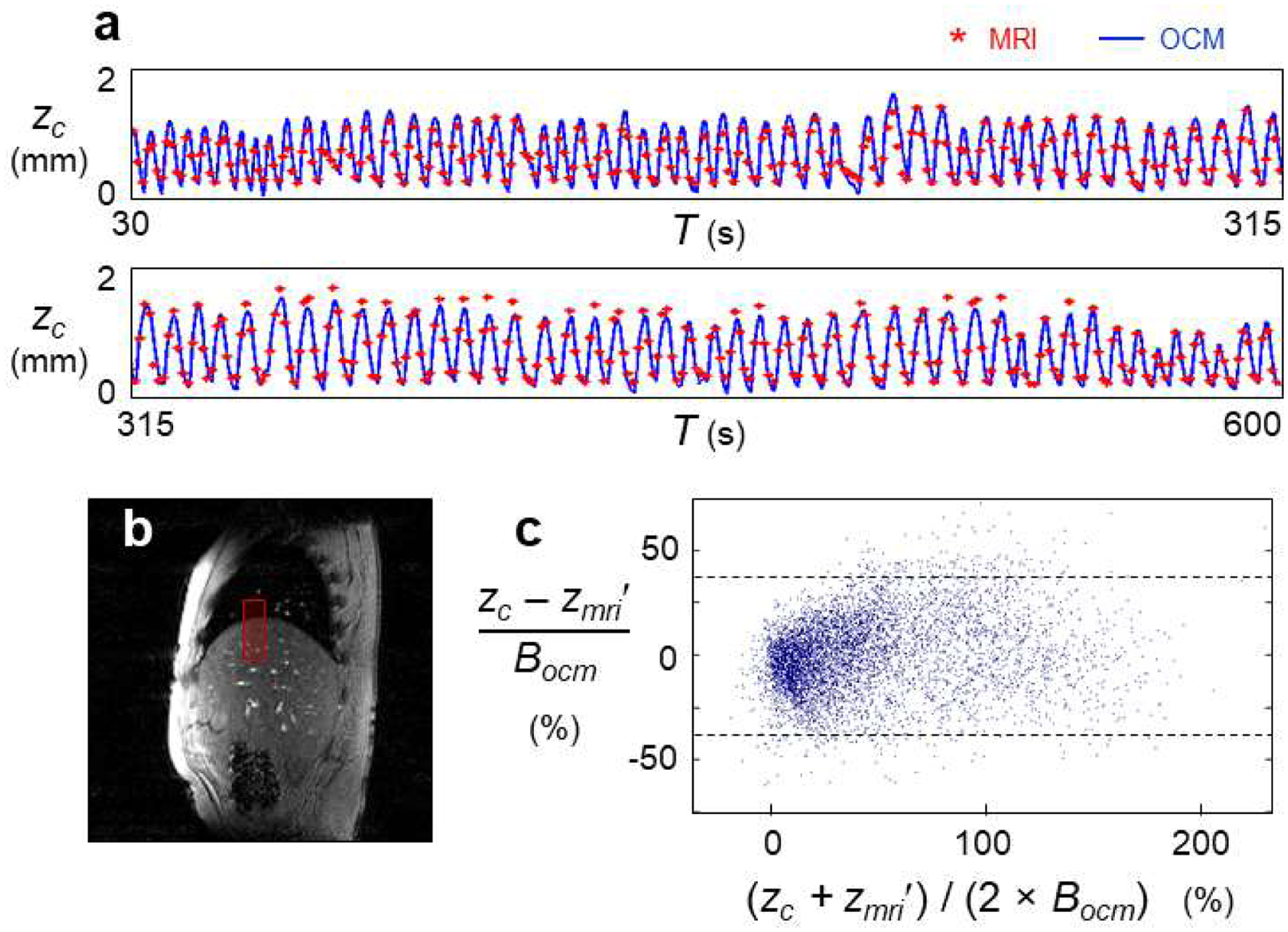
Validation of OCM breathing waveforms against MRI-based measurements. a) Simultaneous OCM and MRI acquisitions were performed in five subjects, leading to 13 separate datasets and 130 min of monitoring. Results are shown in (a) for a typical datasets, i.e., for the dataset with median error. The 570 s display was broken into two rows, for better visibility. b) MRI-based measurements were obtained by placing an ROI over the right hemi-diaphragm, and displacements in the superior-inferior direction were linearly scaled to fit the OCM-derived waveform (first MRI frame for Subject A2 shown here). c) OCM-based and MRI-based results were compared, for all data from all subjects (i.e., Subjects A1 through A5). z_mri′ is the version of z_mri that was brought to the same scale as z_c, and comparison results in (c) were normalized by a ‘typical breath’ B_ocm = 0.84 mm, see text for details. Dashed lines show the 95% limits of agreement, which were 70.2% apart. The mean absolute error was 13.1%.

C. Validation of OCM waveforms against optical tracking

Simultaneous optical tracking and OCM monitoring were performed with a ceiling-mounted tracking system used clinically for radiotherapy treatment planning, along with OCM sensors fixed to both abdomen and chest (see Fig. 1b), on eight volunteers referred to as Subjects B1 through B8. Three 5-min acquisitions per subject were processed using the exact same causal algorithm and settings as for the MRI validation above. Linear scaling was applied to each 5-min optical tracking waveform to fit the scale of the corresponding OCM-derived result. In some cases, such as Fig. 3a (Subject B5, 3^rd dataset out of 3), the OCM-derived and optical tracking waveforms were nearly identical. A typical case, i.e., the case with median error, is shown in Fig. 3b (Subject B1, 2^nd out of 3). The comparison between OCM-based waveforms, z_c, and corresponding optical tracking results, z_opt, is shown in Fig. 3c for all data from subjects B1 through B8. Results were normalized by B_ocm and presented here as a percentage value. Dashed lines show the 95% limits of agreement, which were 101% apart, and the mean absolute error was 15.5%.

Figure 3:

Validation of OCM breathing waveforms against optical tracking measurements. a,b) Simultaneous OCM and optical tracking acquisitions were performed in eight subjects, leading to 24 separate datasets of 5 min each. In some datasets (e.g., (a)) the two waveforms were nearly identical. The dataset with median error is shown in (b). c) OCM-based and optical tracking result were compared for all data from all subjects (i.e., Subjects B1 through B8). The display shows the density of points rather than individual points because of the large number of points involved. z_opt′ is the version of z_opt that was brought to the same scale as z_c, and comparison results in (c) were normalized by a ‘typical breath’ B_ocm = 0.84 mm, see text for details. Dashed lines show the 95% limits of agreement, which were 101% apart. The mean absolute error was 15.5%.

D. Available by OCM but not otherwise: depth and chest motion

Abdominal motion at three separate depths is plotted in Fig. 4a and 4b for Subject A5 (4^th dataset out of 6) and Subject B4 (1^st out of 3), respectively. The amplitude of abdominal motion detected at all three depths is shown in Fig. 4c, whenever available, for all 37 datasets from all 13 subjects that were recruited here.

Figure 4:

Breathing waveforms as a function of tissue depth. a,b) For several subjects, such as Subject A5 shown in (a), waveforms at different depths differed mostly in terms of motion amplitude, with larger motion detected at deeper locations. In contrast, for Subject B4 shown in (b), deeper tissues moved in the opposite direction relative to shallower subcutaneous tissues. c) Motion amplitude is shown for all 37 datasets obtained in 13 volunteers, and useful depth information was obtained in all subjects but A3, B5 and B8.

While Subjects A1–A5 had only a single OCM sensor on the abdomen, subjects B1–B8 had a second OCM sensor attached to their chest. This chest sensor was placed over the heart, which is protected by the ribs and surrounded by the lungs. Because US waves are strongly reflected by both bones and air, reflections were expected and embraced; as such, any attempt to think of the t axis as ‘depth’ might be misguided in this case. For this reason, and unlike abdominal signals (Fig. 4), the chest signals were processed into a single waveform based on the entire t axis. Chest motion is shown in Fig. 5a for Subject B2 (3^rd dataset out of 3) and in 5b for Subject B8 (2^nd out of 3). All available chest-related information is summarized in Fig. 5c, which shows the motion amplitude for all datasets from Subjects B1–B8 whenever possible. While Fig. 5a and 5b compare data from abdominal and chest sensors, data in Fig. 5c comes from chest sensors only.

Figure 5:

Characterizing the breathing-related chest motion. a,b) Datasets were obtained from Subjects B1 through B8 while breathing naturally, while emphasizing abdominal breathing, and while emphasizing chest breathing. For most volunteers, such as Subject B2 in (a), chest and abdominal motion were mostly in sync while emphasizing chest breathing. In contrast, phase offsets were often present when subjects were asked to emphasize abdominal breathing, with Subject B8 in (b) an extreme example as chest and abdominal motion were almost entirely out of phase. c) For all subjects for whom reliable chest motion estimates were available for both abdominally- and chest-emphasized acquisitions (B2 through B6), chest motion had greater amplitude on the latter, as could be expected.

Discussion

There are three main points being made through the present work: OCM signals include the information readily obtained by optical tracking and/or MRI monitoring of breathing motion (Figs. 2 and 3), OCM signals capture further information (Figs. 4 and 5), and OCM sensors can follow a given patient through diagnostic and therapeutic procedures that are separated in time and space. The processing strategy presented here involved using the phase of OCM signals to measure displacements waveforms (Eqs. 1–3), and the magnitude, envelope-detected signals to detrend these waveforms (Eqs. 4–8). The processing was fully automated, in the sense that it did not require any human selection/input. While diagnostic scanners and/or optical trackers mounted to floors or ceilings can be employed only when a patient shares their space, OCM R2.1 sensors are attached to the skin and can accompany a patient, potentially acting as a bridge through multiple procedures. For procedures on separate days, sensors would have to be detached/re-attached to the same spot(s) on the skin.

For all 13 subject (A1–A5 and B1–B8), useful breathing waveforms were obtained from the shallowest depth range (< 3.3 cm) from a sensor placed on the abdomen, and these waveforms were used for validation against MRI and optical tracking (Figs 2 and 3). These shallow signals came from subcutaneous tissues and were due to the slight compression/expansion of these tissues with breathing, as they moved with respect to the skin surface and the OCM sensor attached to it. Quality signals from greater depths and from the chest sensor were available in most volunteers but not all: 10 out of 13 had useful depth information (all but Subjects A3, B5 and B8, see Fig. 4c), and 5 out of 8 had useful chest motion information (all but Subjects B1, B7 and B8, see Fig. 5c). As could be expected, abdominal motion tended to be greatest when subjects were instructed to emphasize abdominal breathing (Fig. 4c, middle grouping for Subjects B1 through B4, B6 and B7), and chest motion tended to be greatest when subjects were instructed to emphasize chest breathing (Fig. 5c, subjects B2–B6).

While motion at different depths and locations often appeared as larger/smaller versions of each other, at times they included features that stood out as reminders of how personal and varied breathing patterns can be, such as the reverse direction of deeper abdominal motion observed in Subject B4 (Fig. 4b) or the out-of-phase nature of chest motion in Subject B8 (Fig. 5b). The fact that Subject B4 was a strong chest breather (see Fig. 5c) may help explain the unusual abdominal motion observed in Fig. 4b. Breathing motion varied from very slow (Fig. 5b) to very rapid (Fig. 5a), and even stopped at times for no apparent reason (Fig. 3a). More generally, while breathing waveforms of a nature similar to those from MRI and optical tracking could be obtained in all volunteers (Fig. 2 and 3), much richer multi-parametric information could be obtained in most but not all volunteers (Fig. 4 and 5). Improved algorithms and/or experience with sensor placement will likely help increase the proportion of people for which richer information can be obtained. The use of machine learning methods to extract information from OCM signals (as explored in our prior work²⁹) remains promising, although such information may prove less intuitive and harder to work into existing motion mitigation and compensation algorithms than the quantitative waveforms generated here.

Limitations of the present study include the relatively small number of volunteers. While all algorithms were causal and as such compatible with real-time processing and display, the actual processing was done offline from OCM, MRI and optical tracking data stored in computer files. The computing of 2-sensor, 3-depth OCM datasets acquired over a period τ took about a processing time of 1.9×τ to complete using non-optimized code running on an off-the-shelf desktop computer (Intel i7-4820K, 3.7 GHz, 64 GB of memory), suggesting that a latency of one time point or less should be quite achievable, as required for real-time display. In applications where real-time processing and display would not be necessary, relaxing the requirement for causality by allowing the algorithm to look at future as well as past time points would in all likelihood improve performance, i.e., it would reduce errors in breathing waveforms obtained from OCM sensors.

A most direct application of the proposed technology would be to provide breathing waveforms to medical and/or therapeutic equipment that perform respiratory gating. The present validation study suggests that, at a minimum, OCM waveforms derived from shallow abdominal tissues could replace waveforms derived from more traditional means, in largely equivalent fashion. However, we hope that superiority, and not only equivalence, might be achieved in future work. Because OCM-derived waveforms provide depth-dependent and position-dependent information, new synthetic waveforms that best blend all this information might be generated, to allow diagnostic and/or therapeutic equipment to hopefully reach their best possible performance in terms of respiratory gating.

Conclusions

The small ultrasound-based sensors presented here can be attached to the skin and provide rich breathing-related information. This information could be used to help prevent image degradation during medical imaging, and/or to create bridges between diagnostic and therapeutic sessions that occur in different places and times.

References

- 1.Wood ML, Henkelman RM. MR image artifacts from periodic motion. Med Phys. 1985;12(2):143–151. [DOI] [PubMed] [Google Scholar]
- 2.Keall PJ, Mageras GS, Balter JM, et al. The management of respiratory motion in radiation oncology report of AAPM Task Group 76. Med Phys. 2006;33(10):3874–3900. [DOI] [PubMed] [Google Scholar]
- 3.Nehmeh SA, Erdi YE. Respiratory motion in positron emission tomography/computed tomography: a review. Seminars in nuclear medicine. 2008;38(3):167–176. [DOI] [PubMed] [Google Scholar]
- 4.Ling CC, Yorke E, Amols H, et al. High-tech will improve radiotherapy of NSCLC: a hypothesis waiting to be validated. International journal of radiation oncology, biology, physics. 2004;60(1):3–7. [DOI] [PubMed] [Google Scholar]
- 5.de Oliveira PL, de Senneville BD, Dragonu I, Moonen CT. Rapid motion correction in MR-guided high-intensity focused ultrasound heating using real-time ultrasound echo information. NMR Biomed. 2010;23(9):1103–1108. [DOI] [PubMed] [Google Scholar]
- 6.Peters NH, Bartels LW, Sprinkhuizen SM, Vincken KL, Bakker CJ. Do respiration and cardiac motion induce magnetic field fluctuations in the breast and are there implications for MR thermometry? J Magn Reson Imaging. 2009;29(3):731–735. [DOI] [PubMed] [Google Scholar]
- 7.Wade OL. Movements of the thoracic cage and diaphragm in respiration. J Physiol. 1953;124:193–212. [DOI] [PMC free article] [PubMed] [Google Scholar]
- 8.Suramo I, Paivansalo M, Myllyla V. Cranio-caudal movements of the liver, pancreas and kidneys in respiration. Acta Radiol Diagn (Stockh). 1984;25(2):129–131. [DOI] [PubMed] [Google Scholar]
- 9.Gay SB, Sistrom CL, Holder CA, Suratt PM. Breath-holding capability of adults. Implications for spiral computed tomography, fast-acquisition magnetic resonance imaging, and angiography. Investigative radiology. 1994;29(9):848–851. [PubMed] [Google Scholar]
- 10.Holland AE, Goldfarb JW, Edelman RR. Diaphragmatic and cardiac motion during suspended breathing: preliminary experience and implications for breath-hold MR imaging. Radiology. 1998;209(2):483–489. [DOI] [PubMed] [Google Scholar]
- 11.Liu YL, Riederer SJ, Rossman PJ, Grimm RC, Debbins JP, Ehman RL. A monitoring, feedback, and triggering system for reproducible breath-hold MR imaging. Magn Reson Med. 1993;30(4):507–511. [DOI] [PubMed] [Google Scholar]
- 12.Ehman RL, Felmlee JP. Adaptive technique for high-definition MR imaging of moving structures. Radiology. 1989;173(1):255–263. [DOI] [PubMed] [Google Scholar]
- 13.Pipe JG. Motion correction with PROPELLER MRI: application to head motion and free-breathing cardiac imaging. Magn Reson Med. 1999;42:963–969. [DOI] [PubMed] [Google Scholar]
- 14.Hess M, Buther F, Schafers KP. Data-Driven Methods for the Determination of Anterior-Posterior Motion in PET. IEEE Trans Med Imaging. 2017;36(2):422–432. [DOI] [PubMed] [Google Scholar]
- 15.Liu C, Alessio AM, Kinahan PE. Respiratory motion correction for quantitative PET/CT using all detected events with internal-external motion correlation. Med Phys. 2011;38(5):2715–2723. [DOI] [PMC free article] [PubMed] [Google Scholar]
- 16.Zhang T, Keller H, O’Brien MJ, Mackie TR, Paliwal B. Application of the spirometer in respiratory gated radiotherapy. Med Phys. 2003;30(12):3165–3171. [DOI] [PubMed] [Google Scholar]
- 17.Santelli C, Nezafat R, Goddu B, et al. Respiratory bellows revisited for motion compensation: preliminary experience for cardiovascular MR. Magn Reson Med. 2011;65(4):1097–1102. [DOI] [PMC free article] [PubMed] [Google Scholar]
- 18.Wagman R, Yorke E, Ford E, et al. Respiratory gating for liver tumors: use in dose escalation. International journal of radiation oncology, biology, physics. 2003;55(3):659–668. [DOI] [PubMed] [Google Scholar]
- 19.Spangler-Bickell MG, Khalighi MM, Hoo C, et al. Rigid Motion Correction for Brain PET/MR Imaging using Optical Tracking. IEEE transactions on radiation and plasma medical sciences. 2019;3(4):498–503. [DOI] [PMC free article] [PubMed] [Google Scholar]
- 20.Zaitsev M, Dold C, Sakas G, Hennig J, Speck O. Magnetic resonance imaging of freely moving objects: prospective real-time motion correction using an external optical motion tracking system. Neuroimage. 2006;31(3):1038–1050. [DOI] [PubMed] [Google Scholar]
- 21.Hughes S, McClelland J, Tarte S, et al. Assessment of two novel ventilatory surrogates for use in the delivery of gated/tracked radiotherapy for non-small cell lung cancer. Radiotherapy and oncology : journal of the European Society for Therapeutic Radiology and Oncology. 2009;91(3):336–341. [DOI] [PubMed] [Google Scholar]
- 22.Chi PC, Balter P, Luo D, Mohan R, Pan T. Relation of external surface to internal tumor motion studied with cine CT. Med Phys. 2006;33(9):3116–3123. [DOI] [PubMed] [Google Scholar]
- 23.Fayad H, Pan T, Pradier O, Visvikis D. Patient specific respiratory motion modeling using a 3D patient’s external surface. Med Phys. 2012;39(6):3386–3395. [DOI] [PMC free article] [PubMed] [Google Scholar]
- 24.Dasari P, Johnson K, Dey J, et al. MRI Investigation of the Linkage Between Respiratory Motion of the Heart and Markers on Patient’s Abdomen and Chest: Implications for Respiratory Amplitude Binning List-Mode PET and SPECT Studies. IEEE Trans Nucl Sci. 2014;61(1):192–201. [DOI] [PMC free article] [PubMed] [Google Scholar]
- 25.Günther M, Feinberg DA. Ultrasound-guided MRI: preliminary results using a motion phantom. Magn Reson Med. 2004;52(1):27–32. [DOI] [PubMed] [Google Scholar]
- 26.Rubin JM, Fowlkes JB, Prince MR, Rhee RT, Chenevert TL. Doppler US gating of cardiac MR imaging. Acad Radiol. 2000;7(12):1116–1122. [DOI] [PubMed] [Google Scholar]
- 27.Schwartz BM, McDannold NJ. Ultrasound echoes as biometric navigators. Magn Reson Med. 2013;69(4):1023–1033. [DOI] [PMC free article] [PubMed] [Google Scholar]
- 28.Preiswerk F, Toews M, Hoge WS, et al. Hybrid Utrasound and MRI Acquisitions for High-Speed Imaging of Respiratory Organ Motion. In: Navab N, Hornegger J, Wells W, Frangi A, eds. Medical Image Computing and Computer-Assisted Intervention – MICCAI 2015. Vol 9349. Springer International Publishing; 2015:315–322. [DOI] [PMC free article] [PubMed] [Google Scholar]
- 29.Preiswerk F, Toews M, Cheng CC, et al. Hybrid MRI-Ultrasound acquisitions, and scannerless real-time imaging. Magn Reson Med. 2017;78(3):897–908. [DOI] [PMC free article] [PubMed] [Google Scholar]
- 30.Preiswerk F, Cheng CC, Luo J, Madore B. Synthesizing dynamic MRI using long-term recurrent convolutional networks. 9th International Conference on Machine Learning in Medical Imaging. 2018. [Google Scholar]
- 31.Preiswerk F, Cheng C-C, Wu P-H, Panych LP, Madore B. Ultrasound-based cardiac gating for MRI. Paper presented at: International Society of Magnetic Resonance in Medicine 2017; Honolulu, USA, p. 4443. [Google Scholar]
- 32.Madore B, Cheng C-C, Preiswerk F. Combining MR and ultrasound imaging, through sensor-based probe tracking. Paper presented at: International Society of Magnetic Resonance in Medicine 2019; Montréal, Québec, Canada, p. 0968. [Google Scholar]
- 33.Madore B, Preiswerk F, Bredfledt J, Zong S, Cheng C-C. Motion monitoring using MR-compatible ultrasound-based sensors. Paper presented at: International Society of Magnetic Resonance in Medicine 2020; p. 0461. [Google Scholar]
- 34.Bushberg JT, Seibert JA, Leidholdt EM, Boone JM. Doppler ultrasound. In: Bushberg JAS Jerrold T., Leidholdt Edwin M. and Boone John M., ed. The essential physics of medical imaging. Philadelphia, PA, USA: Lippincott Williams & Wilkins, a Wolters Kluwer business; 2012:542–554. [Google Scholar]