Soft-tissue spectral subtraction improves transcutaneous Raman estimates of murine bone strength in vivo

Abstract

Transcutaneous determination of a bone’s Raman spectrum is challenging because the type I collagen in the overlying soft tissue is spectroscopically identical to that in bone. In a previous transcutaneous study of murine tibiae, we developed a library-based model called SOLD to unmix spatially-offset Raman measurements into three spectra: a bone estimate, a soft tissue estimate, and a residual. Here, we demonstrate the value of combining the bone estimate and the residual to produce a “top layer subtracted” (tls) spectrum. We report superior prediction of two standard bone metrics (volumetric bone mineralization density and maximum torque) using partial least squares regression models based upon tls spectra rather than SOLD bone estimates, implying that the spectral residuals contain useful information. Simulations reinforce experimental in vivo findings. This chemometric approach, which we denote as SOLD/TLS, could have broad applicability in situations where comprehensive spectral libraries are difficult to acquire.

Graphical Abstract

[We adapt a library-based model called SOLD to unmix spatially-offset Raman measurements of murine tibiae in vivo to produce a "top layer subtracted" (tls) spectrum. Superior prediction of volumetric bone mineralization density and maximum torque using partial least squares regression on tls spectra rather than the SOLD spectra is reported. Simulations indicate this chemometric approach could have broad applicability when comprehensive spectral libraries are difficult to acquire.]

1 ∣. INTRODUCTION

By 2025, osteoporosis will cause more than 3 million bone fractures per year^[1]. A key to preventing these fractures is accurately diagnosing osteoporosis in an early stage. Bone properties such as areal bone mineral density (aBMD) or volumetric bone mineralization density (vBMD) measured by dual-energy X-ray absorptiometry (DXA) and X-ray computed tomography (CT) respectively can be used to estimate bone fragility and the risk of fracture. However, DXA has been shown to be less sensitive for diagnosing low bone quality in osteoporotic and obese subjects^[2]. Alternatively, vBMD is a more accurate predictor for low bone quality^[3], but the accuracy of CT is dependent on the amount of radiation used. Large and repeated doses of radiation have been shown to have a negative effect on subjects^[4,5]. Magnetic resonance imaging can measure bone mineral density by imaging the whole musculoskeletal system^[6]. However, it is not widely used clinically due to the high cost. A recently developed technique, reference point indentation (RPI), can assess bone toughness in a minimally invasive manner^[7] and yet its theoretical potential to be applied in vivo is still to be determined^[8]. Ex vivo whole-bone mechanical tests, such as torsion testing and three-point bending, apply loads to create fractures and assess the bone strength^[9] which are not viable as clinical diagnostics.

On the other hand, bone quality is related to the chemical composition^[10]. Raman spectroscopy is a non-invasive tool that can assess the bone’s chemical structure. It has been used to measure the mineral and organic matrix components of bones and further assess phosphate mineralization and bone health ex vivo^[11-13]. In addition, by using spatially offset Raman spectroscopy (SORS), transcutaneous measurements can be obtained with increased specificity to bone in vivo^[14-19]. Our group has shown that transcutaneous Raman signals from SORS are significantly correlated to aBMD, vBMD, and bone strength measured by torsion testing defined as maximum torque (MT), using partial least squares regression (PLSR)^[20].

Although SORS increases specificity to deeper regions of a sample, the spectra still contain signal from the upper region. In the case of transcutaneous measurements of bone, both the soft tissue and the bone contain a prominent contribution from type I collagen. Estimating the target component’s intrinsic Raman spectrum in the presence of such a contaminant is a challenge to which several multivariate techniques have been applied, including band-target entropy minimization (BTEM)^[21-23], multivariate curve resolution^[24], and parallel factor analysis (PARAFAC)^[25]. In particular to bone, these three methods were applied to SORS data and their performance showed the capability of reconstructing phosphate-to -carbonate and mineral-to-matrix ratios^[16].

Our group recently developed a method called simultaneous overconstrained library-based decomposition (SOLD) to convert transcutaneous measurements into basis spectra of bone and soft tissue for the measured region^[26]. Using this method, spectra of mouse tibiae estimated from intact-limb measurements were significantly correlated with the corresponding spectra of the same bones measured ex vivo. In that study, SOLD produced its estimates using two experimentally-obtained spectral libraries, one of bone specimens and one of soft tissue specimens. Spectral fits to transcutaneous spectra exhibited insignificant residuals other than shot noise.

Here, we generalize to cases where the bone library fails to span the full range of bones that are encountered transcutaneously, and is thus unable to fit all spectral features. Using simulated and experimental datasets, we demonstrate that the new method is more robust than SOLD both in preserving spectral peak ratios and in correlating to chemical and mechanical reference measurements.

2 ∣. METHODS

2.1 ∣. Theory

2.1.1 ∣. SOLD

The SOLD algorithm^[26] assumes that each specimen contains two “pure” materials (the target and the contaminant) with different Raman spectral lineshapes (basis spectra). Throughout the optically explored volume, the materials’ lineshapes are invariant, but the relative concentration of the two materials is spatially heterogeneous. For narrative purposes we will refer to two separate homogeneous layers (contaminant on top, target below), but the method works for other types of heterogeneity. We denote the target’s normalized basis spectrum as b_b (subscript meaning “bottom”), and the contaminant’s equivalent as b_t (“top”). We emphasize that different specimens will in general have different b_b and b_t spectra. SOLD’s goal is to produce estimated basis spectra ${\widehat{\mathbf{b}}}_{\mathrm{b}}$ and ${\widehat{\mathbf{b}}}_{\mathrm{t}}$ for each specimen that are as close as possible to the true b_b and b_t.

Multiple epi-detected measurements are obtained with different source-detector offsets, as shown in Figure 1. The banana shapes, conceptually representing the most-explored region for each source-detector pair, emphasize that the relative sampling of the target and contaminant regions changes with separation. SOLD assumes that the total Raman spectrum for each separation is a weighted sum of b_b and b_t, with different offset measurements having different relative weights. To analyze a two-material sample, at least two different source-detector separations are needed.

FIGURE 1.

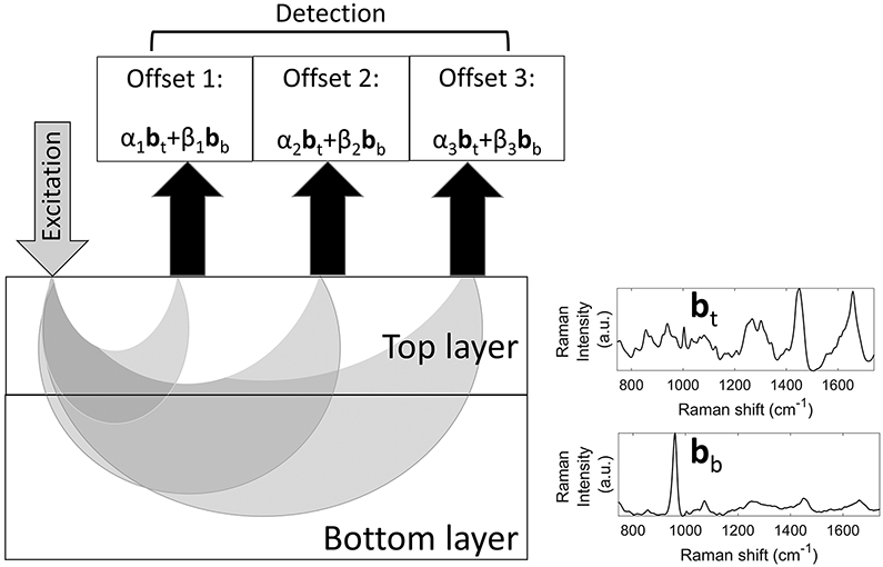
Geometry of spatially-offset Raman spectroscopy measurements (aspect ratio not rendered to scale). Each detected signal is a weighted sum of the top (contaminant) and bottom (target) layers’ basis spectra (b_t and b_b, respectively), with the weight coefficients α and β varying differently with source-detector separation.

SOLD builds the estimates ${\widehat{\mathbf{b}}}_{\mathrm{b}}$ and ${\widehat{\mathbf{b}}}_{\mathrm{t}}$ using two previously-acquired spectral libraries, one of targets and one of contaminants. Each transcutaneous spectrum t can then be modeled as

$${\mathbf{t}}_i={\alpha }_i{\widehat{\mathbf{b}}}_{\mathrm{t}}+{\beta }_i{\widehat{\mathbf{b}}}_{\mathrm{b}}+{\mathbf{e}}_i,$$ (1)

where i is the index for different offsets, α and β are weight coefficients, and e_i is the spectral residual of the fit. SOLD requires at least as many offsets as the number of pure materials. The iterative fitting process imposes a physical constraint on the use of the libraries: the weight coefficients for building ${\widehat{\mathbf{b}}}_{\mathrm{b}}$ and ${\widehat{\mathbf{b}}}_{\mathrm{t}}$ must all be nonnegative.

2.1.2 ∣. SOLD/TLS

As previously noted, the two spectral libraries in the initial test of SOLD were able to model the SORS data to within the shot noise. Such performance cannot always be ensured, for numerous reasons. For example, access to suitable specimens in the library-building phase may be limited; novel sample types may be encountered after library-building is completed; or calibration transfer between spectrographs may introduce biases.

If libraries cannot model the data to within the shot noise, then spectral features from the samples will appear in the spectral residuals e_i of Equation 1. In this scenario, it is unclear what spectrum is most valuable to regress against bone reference values. Should one still use the SOLD estimate ${\widehat{\mathbf{b}}}_{\mathrm{b}}$? Or should one include the features in the residual as well, on the premise that bone information might be added? The answer will vary depending upon the main cause of the modeling imperfection. In the particular application to bone analysis, if the bone library were lacking in scope, the bone estimate from SOLD would be imperfect, and at least some of the sample’s true bone spectrum would likely wind up in the residual, e.

Adding the bottom-layer estimate and the residual spectrum is equivalent to subtracting the top-layer estimate from the original SORS spectrum. We therefore name this quantity the SOLD/TLS spectrum, or tls (“top layer subtracted”) for short, and define it mathematically as

$$\mathbf{tls}\equiv {\mathbf{t}}_{\mathbf{max}}-{\alpha }_{\mathbf{max}}{\widehat{\mathbf{b}}}_{\mathrm{t}}={\beta }_{\mathbf{max}}{\widehat{\mathbf{b}}}_{\mathrm{b}}+\mathbf{e},$$ (2)

where t_max is the SORS measurement with the largest source-detector offset. This measurement is chosen because it has largest specificity to the bottom (target) layer.

We emphasize that the SOLD/TLS approach still uses the bone library but no longer assumes that it produces a faithful estimate of the true b_b. Instead, it only assumes that the estimate of the contaminant’s spectral contribution is reasonably accurate, enough to provide an advantage by subtracting it. The remaining signal is a combination of ${\widehat{\mathbf{b}}}_{\mathrm{b}}$ – guided only by the information in the target library – and any distinctive properties of the sample itself, guided by the experimental measurement.

2.2 ∣. Experimental Data and Analysis

The experimental data presented here were acquired in a previous study^[20]. Briefly, C57BL/6J and B6(Cg)-Tyrc-2J/J mice between the ages of 4 and 23 weeks, 40 mice in total were anaesthetized for in vivo Raman measurements. 150 mW of 830 nm laser light was focused to a spot of 230 μm in diameter on skin overlying the medial midshaft of the right tibia for 300 s. The overlying soft tissue was 1 mm thick on average. Raman scattering was gathered from three annular regions centered upon the excitation spot location, with mean diameters (i.e. source-detector separations) increasing from 0.2 to 0.5 mm. After the in vivo Raman measurements were performed, the mice were sacrificed and the right tibiae were excised and harvested for ex vivo μCT, DXA, and torsion testing. Details for the spectral pre-processing protocol have also been discussed previously^[20]. Briefly, spectral pre-processing included cosmic ray removal, detector readout and dark current subtraction, and image aberration correction. For the updated analysis presented here, spectra from seven mice were removed due to an unexplained and strong fluorescence feature in the 1480-1630 cm⁻¹ range. For the remaining 33 samples, the broad spectral background was suppressed using a fifth-order polynomial linear least-squares fit. Unlike in our previous analysis, the spectral baseline was not flattened by a continuous wavelet transform; this resulted in some negative pixel values but minimized alterations to the Raman spectral bands. All fluorescence-corrected spectra $I_{\tilde{v}}$ were normalized to set the mean absolute deviation (MAD) to unity, i.e.

$$\frac{1}{n}\sum _{i=1}^n\mid S_i-\overline{S}\mid =1.$$ (3)

Separately, Raman spectra were acquired to develop spectral libraries for the SOLD/TLS process, to be described below. 108 ex vivo murine bones, both tibiae and femurs from various genotypes at various ages, were scanned to develop the bone library. Measurements were performed along the medial side of the mid-diaphysis spaced 1 mm apart and averaged. 165 soft tissue samples (including many examples of leg muscle, cartilage, skin, and fat) were acquired ex vivo to develop the soft tissue library.

2.2.1 ∣. Bone property predictions

PLSR^[27] was used to predict bone properties from the transcutaneous Raman spectra (as well as from the simulations described in the next section). There were three bone properties measured by reference methods (aBMD, vBMD, and MT) and four matrices of 33 Raman spectra produced (transcutaneous offset 3, SOLD bone estimates, SOLD/TLS spectra, and for completeness the SOLD soft tissue estimates). Each spectral matrix was regressed against each bone property separately, for a total of twelve leave-one-out cross-validations. In each cross-validation step, the PLSR model rank was set objectively, using the F-statistic to choose the lowest rank without under-calibrating (as described in^[27]) and in all cases going no higher than 1/3 the total sample size to avoid overfitting^[28].

2.3 ∣. Simulations

To enable comparison of SOLD/TLS to standard SOLD under controlled conditions, simulated b_b and b_t spectra were conjured from the spectral libraries. Two sets of six randomly-selected spectra from the bone and soft tissue libraries were randomly weighted to create 33 different [b_b, b_t] pairs, matching the number of samples in the experiment. These basis spectra enabled simulation of SORS data from 33 samples, as will be described further below. Multiple spectral datasets were simulated by repeating the entire process. The remaining 102 bone spectra and 159 soft-tissue spectra in each iteration served as independent libraries to fit the simulated SORS data.

The differences between SOLD and SOLD/TLS spectra produced from these simulated datasets were quantified in two ways. To measure purely spectroscopic effects, the ratio of two spectral peaks were calculated. To measure the effect upon chemometric predictions, a simulated chemical constituent of bone (henceforth “chemical X”) was added to bones and its concentration was predicted using PLSR. These two studies are described below.

2.3.1 ∣. Spectral fidelity test

We chose to investigate the preservation of phosphate mineral (924-986 cm⁻¹) to amide I matrix (1596-1730 cm⁻¹) ratio (MTMR), a common ex vivo metric related to the relative degree of bone mineralization. As noted earlier, the intrinsic MTMR of the bone is heavily altered in a transcutaneous measurement by the collagen in the overlying soft tissue.

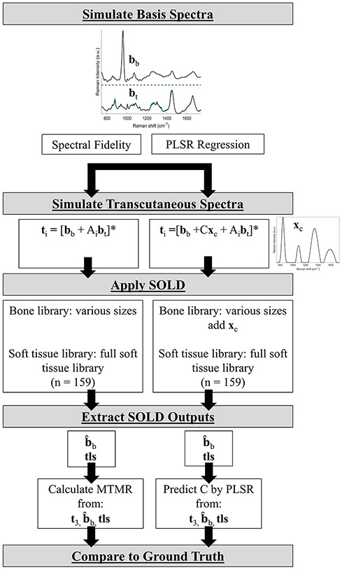
To perform this study, 33 pairs of basis spectra [b_b, b_t] for bottom and top layers were simulated as described above. As illustrated in the lefthand flowchart of Figure 2, SORS data were then simulated for source-detector offsets i = 1, 2, 3 by adding different multiples A_i of b_t to one unit of b_b and then normalizing each sum by its MAD. The simulated transcutaneous (t₃) datasets were designed to have the same mean and standard deviation as the experimental one, corresponding to a “A” range of 0.5-2.5.

FIGURE 2.

Simulation flow chart showing how transcutaneous spectra and SOLD libraries were determined.

*: indicates normalization to MAD.

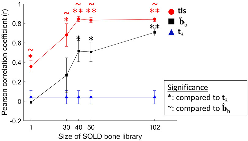
The bone library’s size was systematically decreased to explore its effect upon the estimate of MTMR using SOLD and SOLD/TLS. Starting from the maximum of all 102 available bones, the library was replaced by random selections of 50, 40, 30, and 1 spectra. The soft tissue library, by constrast, was held constant at the full 159 spectra. For each of these simulation runs the MTMR was calculated four ways, using the simulated bone basis spectrum b_b (the true value), the transcutaneous spectrum t₃, the SOLD estimate ${\widehat{\mathbf{b}}}_{\mathrm{b}}$ and the SOLD/TLS estimate tls. The simulation was run 10 times for each SOLD bone library size.

2.3.2 ∣. PLSR regression test

In our experimental work, the spectral variation between different bone spectra is a small fraction of the total signal strength, yet valuable correlations with vBMD and MT have been obtained^[20]. To replicate this in simulation, we imagined a target species, “chemical X”, whose fictional spectrum x_c, shown in Figure 2 , was added at low relative amplitudes C to the bone basis spectrum b_b as SORS data were simulated. This process is depicted in the righthand flowchart of Figure 2. SORS spectra were again normalized to their MAD. C values were set at a low level such that the normalization was minimally influenced by chemical X’s presence. Bone spectra in the SOLD fitting library similarly were given small random amounts of chemical X. SOLD was then conducted, and the concentrations were predicted three times, using PLSR against datasets of t₃, ${\widehat{\mathbf{b}}}_{\mathrm{b}}$ and tls.

We investigated the two limits of the bone library size: the full size of N = 102, and the extreme of a single-bone library. In the latter case, the SOLD bone estimate would be identical for all samples and would therefore have zero predictive power.

Additionally, we simulated an increase in the variability and maximum amplitude of the soft tissue contribution to SORS spectra. This was explored because such amplitudes would occur if the upper layer were thicker, for example for many transcutaneous access points on humans.

2.4 ∣. Statistical Analysis

2.4.1 ∣. Simulation

To measure the ability to preserve Raman peak ratios, the Pearson correlation coefficient r was calculated to compare the MTMR calculated from t₃, ${\widehat{\mathbf{b}}}_{\mathrm{b}}$ or tls to the MTMR from b_b. The Fisher Z-Transform^[29] was used to make the correlation coefficients normally distributed and then the Tukey-Kramer honestly significant difference (HSD) multiple comparison test was used to determine significant differences in Fisher Z values^[29]. Calculations were performed using JMP (Version 15, SAS Institute, Cary, North Carolina).

To compare the accuracy of linear regression against a reference measurement, the root mean squared error of cross validation (RMSECV) and the correlation coefficient were calculated. The raw RMSECVwas divided by the standard deviation of the reference values themselves to give a normalized RMSECV, which we define here as

$$\mathit{v}=\frac{\mathit{RMSECV}}{\frac{\sqrt{{\sum }_{n=1}^N(\overline{y}-y_i{)}^2}}{N}}.$$ (4)

A ν value of 1 conveys that the predictions give essentially no advantage over guessing the mean for all samples. Again, the Tukey-Kramer HSD multiple comparsion test was used to determine significant differences in the ν values.

2.4.2 ∣. Experiment

To check whether experimental bone properties vBMD and MT were predicted better using tls instead of t₃ spectra, we used a bootstrapping approach to offset the small number of samples. 22 of the 33 samples were selected at random and analyzed via cross-validation in the same manner as the full dataset; this random-sampling process was repeated a total of seven times. Significance in the difference in RMSECV values resulting from tls and t₃ spectral input was calculated using a Wilcoxon rank sum test.

3 ∣. RESULTS

3.1 ∣. SOLD/TLS spectra

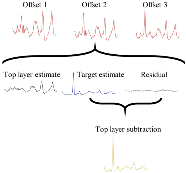
Figure 3 depicts a representative SOLD/TLS spectrum calculation from the transcutaneous, in vivo measurements on mice. First, the SOLD algorithm operated upon a matrix of three SORS spectra from a mouse leg to derive ${\widehat{\mathbf{b}}}_{\mathrm{b}}$ and ${\widehat{\mathbf{b}}}_{\mathrm{t}}$ from spectral libraries of each tissue type. The figure depicts how the largest-offset spectrum, t₃, was decomposed into a weighted sum of ${\widehat{\mathbf{b}}}_{\mathrm{b}}$ and ${\widehat{\mathbf{b}}}_{\mathrm{t}}$, along with a residual. The sum of the bone estimate and the residual then produced the spectrum tls, as given by Equation 2.

FIGURE 3.

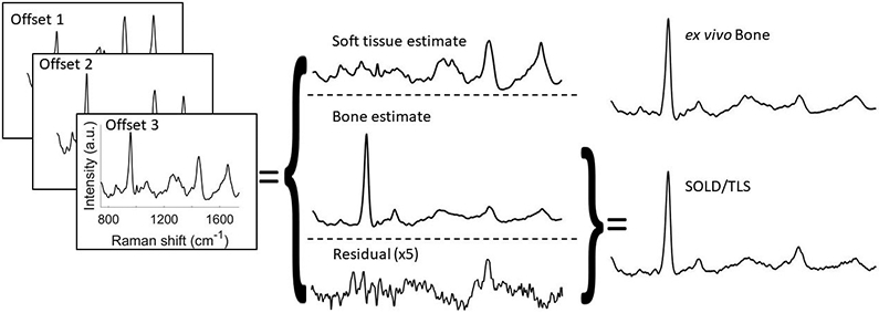
Depiction of SOLD/TLS implementation. Three measured SORS spectra are fed into SOLD, which computes estimated basis spectra ${\widehat{\mathbf{b}}}_{\mathrm{b}}$ and ${\widehat{\mathbf{b}}}_{\mathrm{t}}$. SORS spectrum t₃ is decomposed into contributions from these two basis spectra and a residual, e. Spectrum tls is obtained by subtracting from t₃ the estimated soft tissue contribution. When the residual has structure above the shot-noise limit, tls retains this structure, but ${\widehat{\mathbf{b}}}_{\mathrm{b}}$ does not.

The tls spectrum contains major peaks from minerals such as phosphate (960 cm⁻¹) and carbonate (1070 cm⁻¹), and from organic matrix vibrations, notably amide III (1250 cm⁻¹), CH₂ (1450 cm⁻¹), and amide I (1665 cm⁻¹). The tls spectrum resembles the independently-measured exposed bone spectrum shown above it, while the transcutaneous t₃ is distorted by the higher organic contribution from the overlying soft tissue.

3.2 ∣. Simulation

3.2.1 ∣. Spectral fidelity test

Figure 4 shows the Pearson correlation coefficients between the estimated MTMR (calculated from t₃, ${\widehat{\mathbf{b}}}_{\mathrm{b}}$ or tls) and the true MTMR (calculated from the bone basis spectrum b_b) as the size of the bone library was varied. When the full library (N = 102) was used, both SOLD and SOLD/TLS far outperformed the t₃ results (p < .0001), and SOLD/TLS significantly outperformed SOLD (p < 0.05). As the bone library size was reduced, however, the standard SOLD advantage over t₃ decreased, losing significance for N = 30 and lower. The SOLD/TLS approach, however, retained its advantage over both methods all the way down to N = 1, i.e. a bone library consisting of a single spectrum.

FIGURE 4.

Comparison of how accurately various estimation methods predicted mineral-to-matrix ratio (MTMR) in multiple sets of 33 simulated samples each. Pearson correlation coefficients are plotted for the t₃, SOLD, and SOLD/TLS approaches, with the latter two’s increasing along with the bone library size. Error bars represent standard error of the mean.

*(p<0.05),**(p<.0001): indicates significance compared to t₃ determined by Tukey-Kramer HSD multiple comparisons performed on Fisher z-transformation values

~ (p<0.05): indicates significance compared to ${\widehat{\mathbf{b}}}_{\mathrm{b}}$ determined by Tukey-Kramer HSD multiple comparisons performed on Fisher z-transformation values

3.2.2 ∣. PLSR regression test

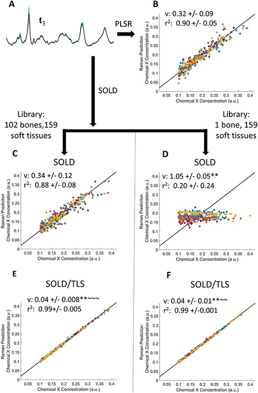
Figures 5 and 6 show the PLSR estimates of chemical X’s concentration using matrices of t₃, ${\widehat{\mathbf{b}}}_{\mathrm{b}}$, or tls spectra and two extreme limits for the bone library’s size: either the full library (N = 102) or a single bone spectrum. In Figure 5 , the spectra were given soft-tissue amplitudes and variation comparable to the levels seen in our experimental data on mouse legs. As Figure 5 A shows, the 33 simulated t₃ spectra all overlap closely, with the most visible variation seen at the phosphate peak. The t₃ PLSR predictions (Figure 5 B), which involved no library, produced a ν of 0.32, i.e. 3X better than guessing the mean of the training concentrations. Using the full library, the SOLD approach produced no better result (Figure 5 C); using the N = 1 library, the SOLD results were useless as expected, essentially guessing the average (Figure 5 D). The SOLD/TLS performance was dramatically better than either other method. Using just the N = 1 library approach, SOLD/TLS produced a ν of 0.04 (Figure 5 F), statistically outperforming both t₃ and full-library SOLD (p < .0001). In this simulation, in fact, SOLD/TLS did not even gain any greater advantage when using the full library (Figure 5 E).

FIGURE 5.

PLSR prediction of simulated trace chemical X concentration, using spectra with soft tissue amplitudes that mimic experimental data. (A) Mean (black line) and standard deviation (blue region) of 33 simulated t₃ spectra. (B–F) PLSR predictions of chemical X concentration using either t₃ spectra (B), ${\widehat{\mathbf{b}}}_{\mathrm{b}}$ spectra (C,D), or tls spectra (E,F). Panels C and E compare results using the full bone library; panels D and F, a library of N = 1. ν and r² are reported as mean +/− standard deviation.

*(p<0.05),**(p<.0001): indicates significance compared to t₃ determined by Tukey-Kramer HSD multiple comparisons

~ (p<0.05), ~ ~ (p<.0001): indicates significance compared to ${\widehat{\mathbf{b}}}_{\mathrm{b}}$ determined by Tukey-Kramer HSD multiple comparisons

FIGURE 6.

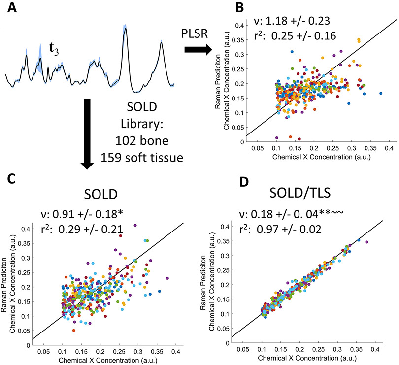
PLSR prediction of simulated trace chemical X concentration using a higher level of soft tissue amplitude variation. (A): Representative set of 33 spectra, showing a less pronounced phosphate peak due to the larger relative amount of soft tissue. (B–D) PLSR predictions using (B) t₃, (C) ${\widehat{\mathbf{b}}}_{\mathrm{b}}$, and (D) tls spectra. ν and r² are represented as mean +/− standard deviation.

*(p<0.05),**(p<.0001): indicates significance compared to t₃ determined by Tukey-Kramer HSD multiple comparisons

~ (p<0.05),~ ~ (p<.0001): indicates significance compared to ${\widehat{\mathbf{b}}}_{\mathrm{b}}$ determined by Tukey-Kramer HSD multiple comparisons

Figure 6 shows the analogous predictions of chemical X when the soft-tissue contribution is varied over a greater range; as noted in section 2.2, the largest amplitude was 8X greater than ever observed in our experimental mouse data. The spectral contribution from phosphate is now much smaller relative to the collagen-related peaks (Figure 6 A, compared to Figure 5 A). Under these more challenging conditions, the predictions using t₃ and full-library SOLD both produced correlation coefficients close to zero (Figure 6 B and C). In contrast, the full-library TLS approach yielded r² = 0.97 (Figure 6 D).

3.3 ∣. Experimental results: bone property predictions

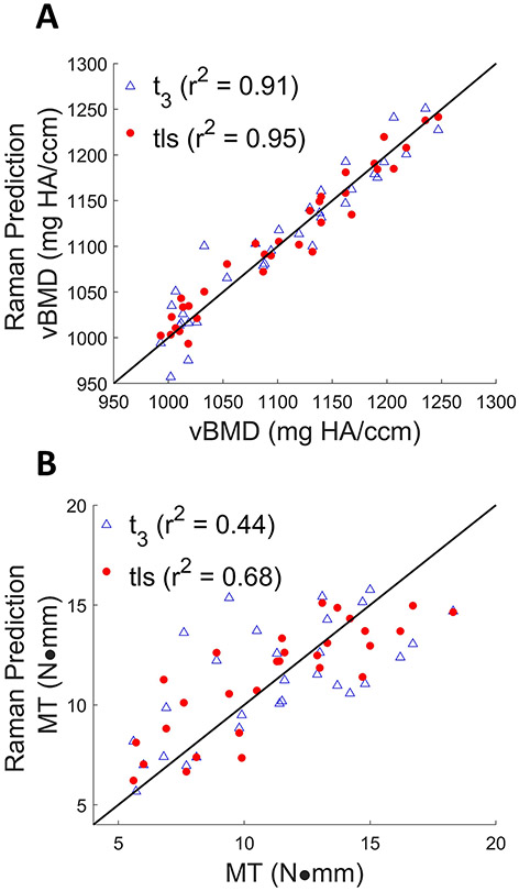
The scatter plots in Figure 7 compare the predictions of vBMD and MT derived from PLSR against either t₃ or tls spectra of 33 mice obtained in vivo. The SOLD/TLS approach produced a lower RMSECV in both cases than t₃ (vBMD errors: 17 vs. 23 mg HA/ccm; MT: 2.0 vs. 2.6 N-mm). The Wilcoxon rank sum test showed that the reductions in RMSECV for both vBMD and MT were significant t₃ (p < 0.05). PLSR predictions of vBMD and MT using either ${\widehat{\mathbf{b}}}_{\mathrm{b}}$ or ${\widehat{\mathbf{b}}}_{\mathrm{t}}$ produced regressions that were inferior to either of the above cases, producing RMSECV values of 39.8 and 65.9 mg HA/ccm for vBMD, and 2.88 and 3.09 for MT, respectively.

FIGURE 7.

Cross-validation results of vBMD (A) measured by μCT using t₃ (marked in blue triangles) (RMSECV = 23.4 mg HA/ccm, r² = 0.91), and tls spectra (marked in red circles) (RMSECV = 17.0 mg HA/ccm, r² = 0.95). Cross validation results of MT (B) measured by torsion testing using t₃(RMSECV = 2.64 N·mm, r² = 0.44), tls spectra (RMSECV = 1.97 N·mm, r² = 0.68). The line of perfect prediction is provided as a guide to the eye; it is not a fit.

For aBMD, the t₃ and tls models yielded the same RMSECV of 0.006 g/cm² and similar r² values of 0.66 and 0.67 respectively (plots not shown). These inferior correlations relative to vBMD (r² of 0.91 and 0.96) will be addressed in the Discussion section.

4 ∣. DISCUSSION

SOLD/TLS combines SOLD’s library-based estimates of the target and interferent materials’ spectral contributions with a sample-specific correction stemming from spectral features that the libraries are unable to model. Subsequent regression models can benefit both from the reduction of superfluous background signal and from the retention of sample-specific information.

In the bone-sensing application used as a test case here, the estimated basis spectra ${\widehat{\mathbf{b}}}_{\mathrm{b}}$ and ${\widehat{\mathbf{b}}}_{\mathrm{t}}$ were modeled empirically using more than 100 bone measurements and 150 soft tissue measurements. As noted previously, a nonnegative weight coefficient constraint was applied to prevent unphysical fits. Despite having more than 100 spectra in each library, we found that many of our transcutaneous spectra could not be modeled to within the shot noise. One possible source of error could be spectral calibration drift between the library-gathering and transcutaneous measurement session. Although the methods used were standard and rigorously applied, calibration transfer in Raman-based regression is a known challenge^[30]. There could also be more fundamental issues pertaining to the samples themselves. The library might not be comprehensive enough to model a particular new bone or soft tissue specimen. In addition, real sample volumes can of course include more than two heterogeneously distributed materials, making it impossible to model three SORS spectra using only two basis spectra, as SOLD assumes. , the intrinsic spectra of Raman scattering and fluorescence are altered by wavelength-dependent absorption variation in the tissue through which they propagate. For the range of wavelengths of interest here, a 5 mm pathlength would impart a variation of less than 10 percent, varying slowly over the width of any individual Raman band. This effect can be mitigated with additional measurements, ^[31,32] but was not corrected here and was not considered in the simulations. All of the above are reasons to anticipate nontrivial spectral residuals when using SOLD.

In our experimental study, we found that the SOLD/TLS method produced the best predictions of two bone properties, volumetric bone mineral density (vBMD) and maximum torque (MT). A priori there was no guarantee that adding the SOLD residual to ${\widehat{\mathbf{b}}}_{\mathrm{b}}$ would improve the predictions. Certainly in general a model’s residual does not have to contain useful information about the reference properties of interest. Had incompleteness in the soft tissue library been the main shortcoming, the SOLD/TLS approach would likely not have improved the bone property predictions. In this particular case, however, the residual did improve the regressions significantly, suggesting that the bone library was limited in its ability to fit some of the transcutaneous bones’ Raman spectra.

The simulation results reinforce this finding that SOLD/TLS provides an advantage when the target library is limited. When the number of samples in the target spectral library was systematically reduced, SOLD/TLS produced higher-fidelity estimates of the target component’s spectrum and more accurate predictions of a trace chemical’s concentration, relative to the t₃ and SOLD approaches.

The conceptual advantage of SOLD/TLS over SOLD becomes clearest in the examples where the target library contained a single spectrum. In this extreme, there was no variation in the calculation of ${\widehat{\mathbf{b}}}_{\mathrm{b}}$ between samples and thus no predictive power for a multivariate regression based upon ${\widehat{\mathbf{b}}}_{\mathrm{b}}$ alone (c.f. Figures 4 and 5 D). Since the unmodeled sample-specific variations wound up in the spectral residual e (c.f. Equation 1), the SOLD/TLS spectra (which incorporate e) were able to produce useful predictions.

In the N = 1 limit, it is not immediately obvious why SOLD/TLS spectra would produce better bone predictions than the transcutaneous spectra t₃, which contain the same sample-specific spectral information. The answer is that the N = 1 libraries, while useless for bone spectrum estimation, did support effective SOLD modeling of the interferent’s spectral contribution. Simply removing the bulk of the soft-tissue signal improved the subsequent predictions, as evidenced in Figures 4 and 5 F. One interpretation is that the soft tissue’s type I collagen contribution confounds the regression process and should thus be subtracted as accurately as possible in postprocessing. As noted in the Introduction, the presence of type I collagen in both soft tissue and bone is known to be a major challenge in transcutaneous Raman-based analysis of bone.

In the regressions performed in this study, all spectra submitted to PLSR were first normalized by their MAD, a measure of the total signal strength. Absolute signal strength from the target material was therefore not retained. This choice was inspired by the particular application to transcutaneous in vivo bone spectroscopy, in which the thickness and optical properties of the overlying soft tissue (varying from sample to sample) significantly perturb the amplitude of the Raman signal detected from bone. Such normalization to total signal strength is relevant to the PLSR reported here. As noted above, variations in bone spectral lineshapes between samples are typically a small percentage of the total bone signal. Because chemical X’s simulated spectral contributions were made similarly small, their variations barely perturbed the MAD normalization. The relationship between X’s concentration and spectral amplitude was therefore nearly linear, with PLSR to predict X’s concentration correspondingly robust. We conjecture that this simulation mimics the experimental conditions under which vBMD is predicted from normalized Raman spectra, although we do not yet have a chemical interpretation of the small-percent variations that correlate with vBMD. We note, however, that were the spectral contributions of chemical X larger, they would more greatly influence the normalization, perturb the linear relationship with concentration, and presumably degrade the predictions. This might be the case in other situations in which SOLD/TLS might be used, and should be taken into consideration.

In addition to demonstrating the general use of SOLD/TLS, this work provides insights about the particular predictions of bone mineral density and maximum torque via Raman spectroscopy. vBMD is derived by analyzing voxels in 3D X-ray images of bone, while aBMD is a 2D measurement that integrates along a line of sight^[33]. The Raman spectroscopy in this study interrogated a fixed volume, and the maximum source-detector separation was only 0.5 mm, less than the typical thickness of the soft tissue layer above the bone. As such, it is likely that the Raman measurement of the bone was at most weakly sensitive to the total tibial thickness, and more closely proportional to the volumetric density. This is borne out in the PLSR predictions, in which higher correlations were found for vBMD than aBMD. Fortunately, vBMD has also been mentioned as a better predictor for bone strength than aBMD^[34].

The MT predictions in this study had lower correlation coefficients than vBMD. vBMD, like Raman spectroscopy, is a direct measurement of the abundance of a chemical within a region. MT, on the other hand, is a mechanical measurement whose relationship to chemical composition is not obviously linear, and which depends upon independent structural properties (e.g. bone cross-sectional area and cortical thickness) that Raman spectroscopy does not probe. As such, a linear regression to predict MT from Raman spectra may well not be the optimal model. In addition, MT measurements are more prone to inconsistencies in setup and handling, leading to greater uncertainty in the reference values. For all of these reasons, the performance of vBMD better exemplifies the key advantages of SOLD/TLS. Nevertheless, improvements were seen for MT as well.

5 ∣. CONCLUSION

We have introduced and tested a new spectral unmixing method based upon SOLD to process in vivo transcutaneous measurements obtained using SORS. By retaining spectral features that are not modeled by SOLD’s fitting library, the SOLD/TLS approach has an advantage when the library fails to model the targeted component’s spectrum completely. In direct comparisons, SOLD/TLS preserved spectral features more faithfully and produced better regressions against reference properties than when unprocessed SORS spectra or traditionally-processed SOLD spectra were used. The experimental application to bone analysis raises the potential of monitoring bone changes in vivo and aiding in the detection of osteoporosis. The SOLD/TLS unmixing approach generalizes to any situation where the SOLD assumptions apply, namely any spatially heterogeneous mixture of N materials in which spatially-offset measurements capture M ≥ N linearly independent superpositions of the materials’ spectral lineshapes.

References

- [1].Burge R, Dawson-Hughes B, Solomon DH, Wong JB, King A, Tosteson A, Journal of Bone and Mineral Research 2007, 22 (3), 465–475. [DOI] [PubMed] [Google Scholar]
- [2].Laskey MA, Nutrition 1996, 12 (1), 45–51. [DOI] [PubMed] [Google Scholar]
- [3].Jergas M, Breitenseher M, Glüer CC, Yu W, Harry K, Genant HK, Journal of Bone and Mineral Research 1995, 10 (7), 1101–1110. [DOI] [PubMed] [Google Scholar]
- [4].Klinck RJ, Campbell GM, Boyd SK, Medical Engineering & Physics 2008, 30 (7), 888–895. [DOI] [PubMed] [Google Scholar]
- [5].Markbreiter LA, Pelker RR, Friedlaender GE, Peschel R, Panjabi MM, Journal of Orthopaedic Research 1989, 7 (2), 178–183. [DOI] [PubMed] [Google Scholar]
- [6].Hong J, Hipp J, Mulkern RV, Jaramillo D, Snyder B, Calcified Tissue International 2000, 66, 74–8. [DOI] [PubMed] [Google Scholar]
- [7].Gallant MA, Brown DM, Organ JM, Allen MR, Burr DB, Bone 2013, 53 (1), 301–305. [DOI] [PMC free article] [PubMed] [Google Scholar]
- [8].Allen MR, McNerny EMB, Organ JM, Wallace JM, Journal of Bone and Mineral Research 2015, 30 (9), 1539–1550. [DOI] [PMC free article] [PubMed] [Google Scholar]
- [9].Silva MJ, Brodt MD, Wopenka B, Thomopoulos S, Williams DD, Wassen MHM, Ko M, Kusano N, Bank R, Journal of Bone and Mineral Research 2006, 21, 78–88. [DOI] [PubMed] [Google Scholar]
- [10].Donnelly E, Clinical Orthopaedics and Related Research 2011, 469 (8), 2128–2138. [DOI] [PMC free article] [PubMed] [Google Scholar]
- [11].Maher JR, Takahata M, Berger AJ, Awad HA, Journal of Biomedical Optics 2011, 16, 16: 087012. [DOI] [PMC free article] [PubMed] [Google Scholar]
- [12].Morris MD, Mandair GS, Clinical Orthopaedics and Related Research 2010, 469, 2160–9. [DOI] [PMC free article] [PubMed] [Google Scholar]
- [13].Makowski AJ, Granke M, Ayala OD, Uppuganti S, Mahadevan-Jansen A, Nyman JS, Appl. Spectrosc 2017, 71 (10), 2385–2394. [DOI] [PMC free article] [PubMed] [Google Scholar]
- [14].Buckley K, Kerns JG, Gikas PD, Birch H, Vinton J, Keen R, Parker AW, Matousek P, Goodship AE, IBMS BoneKEy 2014, 11, 1–3. [Google Scholar]
- [15].Buckley K, Kerns JG, Vinton J, Gikas PD, Smith C, Parker AW, Matousek P, Goodship AE, Journal of Raman Spectroscopy 2015, 46 (7), 610–618. [DOI] [PMC free article] [PubMed] [Google Scholar]
- [16].Buckley K, Kerns JG, Parker AW, Goodship. AE, Matousek P, Journal of Raman Spectroscopy 2014, 45 (2), 188–192. [DOI] [PMC free article] [PubMed] [Google Scholar]
- [17].Esmonde-White FWL, Morris MD, in Photonic Therapeutics and Diagnostics IX, International Society for Optics and Photonics, SPIE, 2013, pp. 810–816. [Google Scholar]
- [18].Dooley M, Prasopthum A, Liao Z, Sinjab F, McLaren J, Rose FRAJ, Yang J, Notingher I, Biomed. Opt. Express 2019, 10 (4), 1678–1690. [DOI] [PMC free article] [PubMed] [Google Scholar]
- [19].Cui H, Glidle A, Cooper JM, IEEE Access 2020, 8, 62905–62911. [Google Scholar]
- [20].Shu C, Chen K, Lynch M, Maher JR, Awad HA, Berger AJ, Biomed. Opt. Express 2018, 9 (10), 4781–4791. [DOI] [PMC free article] [PubMed] [Google Scholar]
- [21].Chew W, Widjaja E, Garland M, Organometallics 2002, 21 (9), 1982–1990. [Google Scholar]
- [22].Ong LR, Widjaja E, Stanforth R, Garland M, Journal of Raman Spectroscopy 2003, 34 (4), 282–289. [Google Scholar]
- [23].Churchwell JH, Sowoidnich K, Chan O, Goodship AE, Parker AW, Matousek P, Journal of Raman Spectroscopy 2020, 51 (1), 66–78. [Google Scholar]
- [24].Ruckebusch C, Blanchet L, Analytica Chimica Acta 2013, 765, 28–36. [DOI] [PubMed] [Google Scholar]
- [25].Bro R, Chemometrics and Intelligent Laboratory Systems 1997, 38 (2), 149–171. [Google Scholar]
- [26].Maher J, Inzana J, Awad Hani H. A., Berger AJ, Journal of Biomedical Optics 2013, 18, 77001. [DOI] [PMC free article] [PubMed] [Google Scholar]
- [27].Wold S, Sjöström M, Eriksson L, Chemometrics and Intelligent Laboratory Systems 2001, 58 (2), 109–130, PLS Methods. [Google Scholar]
- [28].Qi D, Berger AJ, Appl. Opt 2007, 46 (10), 1726–1734. [DOI] [PubMed] [Google Scholar]
- [29].Fisher RA, Biometrika 1915, 10 (4), 507–521. [Google Scholar]
- [30].Pence I, Mahadevan-Jansen A, Chemical Society Reviews 2016, 45 (7). [DOI] [PMC free article] [PubMed] [Google Scholar]
- [31].Shih WC, Bechtel KL, Feld MS, Opt. Expres 2008, 16 (17), 12726–12736. [DOI] [PMC free article] [PubMed] [Google Scholar]
- [32].Bechtel KL, Shih WC, Feld MS, Opt. Express 2008, 16 (17), 12737–12745. [DOI] [PMC free article] [PubMed] [Google Scholar]
- [33].Khoo BCC, Brown K, Cann C, Zhu K, Henzell S, Low V, Gustafsson S, Price RI, Prince RL, Osteoporosis International 2009, 20 (9), 1539–1545. [DOI] [PubMed] [Google Scholar]
- [34].Dall’Ara E, Pahr D, Varga P, Kainberger F, Zysset P, Osteoporosis International 2011, 23, 563–572. [DOI] [PubMed] [Google Scholar]
- [35].Satterthwaite FE, Biometrics Bulletin 1946, 2 (6), 110–114. [PubMed] [Google Scholar]
- [36].Fouladi RT, Steiger JH, Communications in Statistics - Simulation and Computation 2008, 37 (5), 928–944. [Google Scholar]
- [37].Hernandez CJ, Keaveny TM, Bone 2006, 39 (6), 1173–1181. [DOI] [PMC free article] [PubMed] [Google Scholar]
- [38].Cole J, van der Meulen M, Clinical Orthopaedics and Related Research 2011, 469, 2139–49. [DOI] [PMC free article] [PubMed] [Google Scholar]
- [39].Tatoń G, Rokita E, Wróbel A, Korkosz M 2013. [Google Scholar]
- [40].Nascimento JMP, Dias JMB, IEEE Transactions on Geoscience and Remote Sensing 2005, 43 (4), 898–910. [Google Scholar]
- [41].Wu CFJ, Ann. Statist 1986, 14 (4), 1261–1295. [Google Scholar]