An open source autocorrelation-based method for fetal heart rate estimation from one-dimensional Doppler ultrasound

Abstract

Objective:

Open research on fetal heart rate (FHR) estimation is relatively rare, and evidence for the utility of metrics derived from Doppler ultrasound devices has historically remained hidden in the proprietary documentation of commercial entities, thereby inhibiting its assessment and improvement. Nevertheless, recent studies have attempted to improve FHR estimation; however, these methods were developed and tested using datasets composed of few subjects and are therefore unlikely to be generalizable on a population level. The work presented here introduces a reproducible and generalizable autocorrelation (AC)-based method for FHR estimation from one-dimensional Doppler ultrasound (1D-DUS) signals.

Approach:

Simultaneous fetal electrocardiogram (fECG) and 1D-DUS signals generated by a hand-held Doppler transducer in a fixed position were captured by trained healthcare workers in a European hospital. The fECG QRS complexes were identified using a previously published fECG extraction algorithm and were then over-read to ensure accuracy. An AC-based method to estimate FHR was then developed on this data, using a total of 721 1D-DUS segments, each 3.75 s long, and parameters were tuned with Bayesian optimization. The trained FHR estimator was tested on two additional (independent) hand-annotated Doppler-only datasets recorded with the same device but on different populations: one composed of 3938 segments (from 99 fetuses) acquired in rural Guatemala, and another composed of 894 segments (from 17 fetuses) recorded in a hospital in the UK.

Main results:

The proposed AC-based method was able to estimate FHR within 10% of the reference FHR values 96% of the time, with an accuracy of 97% for manually identified good quality segments in both of the independent test sets.

Significance:

This is the first work to publish open source code for FHR estimation from 1D-DUS data. The method was shown to satisfy estimations within 10% of the reference FHR values and it therefore defines a minimum accuracy for the field to match or surpass. Our work establishes a basis from which future methods can be developed to more accurately estimate FHR variability for assessing fetal wellbeing from 1D-DUS signals.

1. Introduction

During pregnancy, fetal cardiac monitoring is a common method for identifying fetal abnormalities in the second and third gestational trimesters (Sandmire and DeMott, 1998). This identification process is performed by examining fetal heart rate (FHR) variations in signals between 10 to 60 minutes, using epochs of 3.75 s as is described in the Dawes/Redman system (Pardey et al., 2002; Dawes et al., 1981). Based on the observable variations, physicians and midwives attempt to identify abnormal patterns indicative of stress or adverse outcomes, in theory facilitating timely intervention if required (Parer et al., 1997; Merz, 2004; Hameed and Sklansky, 2007).

The most common method to monitor FHR and uterine contractions is using Doppler ultrasound devices. These devices use a transducer to measure the change in frequency of a reflected acoustic wave from an object moving relative to the acoustic source. In the case of FHR monitoring, the change of frequency is caused by cardiac wall and valve movements, and sometimes blood flow. These physical movements are recorded as a one-dimensional ultrasound (1D-DUS) signal, which is demodulated into an audio recording so that the operator of the device can hear the resultant heart beat changes in the range of human hearing. This ‘sound’ can then be analyzed to estimate FHR, much like any other cardiac signal. To achieve this, Doppler ultrasound devices use autocorrelation (AC)-based approaches, in an attempt to identify the dominant frequency in a given band (or delay window).

Although Doppler ultrasound devices have been widely used for decades to estimate FHR, one of their limitations is that commercial monitoring companies have not disclosed the details of the algorithms such that ‘someone skilled in the art’ could actually reproduce the exact approach (Marzbanrad et al., 2018). Therefore, the accuracy of Doppler-based FHR estimation systems remain unknown and replication or improvement of such approaches is entirely inhibited.

Despite the difficulty of accessing the FHR estimation source code, relatively little research has been published concerning improving Doppler-based FHR estimation (Jezewski et al., 2008, 2011; Peters et al., 2004; Roj et al., 2010). The majority of publications on this topic that do exist were aimed at improving FHR estimations by comparing the proposed method to estimations provided by direct scalp fECG taken from the fetal head during labor. Although these methods used an accepted reference methods with which to compare their results, they had some limitations. Specifically, they developed and tested their methods using only one dataset composed of only a few patients (between 1 to 15) (Jezewski et al., 2008, 2011; Peters et al., 2004; Roj et al., 2010), optimizing parameters for their specific dataset without holding out data for validation, making it highly unlikely that the developed algorithms would have any generalizability beyond the small number of individuals studied (Liu et al., 2016).

In addition to AC-based methods, in recent years, researchers have also proposed a different approach to estimate FHR from 1D-DUS signals. Specifically, Al-Angari et al. proposed the use of empirical mode decomposition (EMD) of the 1D-DUS signals and the kurtosis of the instantaneous mode function (IMF) as a measure of FHR (Al-Angari et al., 2017). This method was trained using abdominal fECG as a reference. The method was developed using a total of 44 1D-DUS signals of one-minute length each individually extracted from healthy single pregnant women within 24 and 42 gestational weeks. The authors presented evidence that the EMD-kurtosis method achieved higher accuracy than AC-based methods, specially for low SNR signals. However, the parameters of this method, such as the number of IMFs and the window size to calculate kurtosis, were optimized using all of the dataset, again leading to likely overfitting on the limited data used.

Therefore, the aim of this work is to develop a reproducible and generalizable AC-based method able to accurately estimate FHR from 1D-DUS taken with an inexpensive hand-held transducer (Stroux, 2016; Stroux et al., 2016) from subjects of different populations. Although AC-based methods are affected by the inherent smoothing or averaging of the autocorrelation (ACF) (Jezewski et al., 2017; Lauersen et al., 1976; Cesarelli et al., 2009), an AC-based FHR estimator remains a computationally inexpensive approach and, if it is confirmed to be accurate to estimate FHR, it can be a valuable first indicator for fetal wellbeing in itself. Moreover, a recent work has shown that an accurate AC-based estimator can be the basis of more advanced analysis to segment 1D-DUS into beat-to-beat segments (Stroux, 2016), from which FHR variability analysis can be performed.

To ensure an accurate FHR estimation, the method was optimized by comparing to FHR obtained from a simultaneously recorded abdominal fECG as a benchmark. After the method was optimized, it was tested on two independent datasets and different populations, and over the second and third trimesters in order to test any dependency on gestational age.

2. Methods

2.1. Databases

This work used three different 1D-DUS databases collected over a period of four years. All signals were acquired using a hand-held 1D-DUS device (AngelSounds Fetal Doppler JPD-100s, Jumper Medical Co., Ltd., Shenzhen, China) with an ultrasound transmission frequency of 3.3 MHz and a digitization sampling frequency of 44.1 kHz, captured using a Samsung S4, S3 mini or S4 mini and stored as uncompressed WAV files at 7056 Kbps (16 bits).

2.1.1. Leipzig University Hospital Database

This dataset, used for training the FHR estimation algorithm in this study, was collected at the Leipzig University Hospital (LUH) in Germany, as part of the study presented in (Andreotti, 2016). The database included data from 16 volunteers with pregnancies between the 20th and 27th week of gestation, including pathological cases such as Inter-uterine growth restriction (IUGR), premature rupture of membranes, or fetal heart failures. The study was approved by the Leipzig University Hospital ethics committee (record 348-12-24092012), and written informed consent was obtained from each patient. For each subject, indirect abdominal fECG, a maternal ECG reference and a 1D-DUS signal were simultaneously recorded by clinicians. The fECG recordings were acquired from 7 abdominal channels using a 16bit commercial ADC using the ADInstruments ML138 Octal Bio Amp and ADInstruments PowerLab 16/30 (ADInstruments, Dunedin, NZ), and stored at a sampling frequency of 1000 Hz. Spectral filtering was also performed in the hardware by a mains filter (cutoff frequency at 50 Hz) and a first-order high-pass filter (cutoff at 1 Hz).

2.1.2. Oxford JR Database

This dataset was collected at the John Radcliffe (JR) Hospital in Oxford, UK. The study was approved by the NHS Health Research Authority (REC reference: 12/SC/0147) and written consent was obtained from each study subject prior to data collection. Each subject received detailed information on the study protocol and their right to withdraw from the study at any stage of the recording session, which was carried out by professional midwives. The dataset included 1D-DUS signals from 17 healthy pregnant women, who bore singletons between 20 and 38 weeks of gestation. This database has also been used in previous related 1D-DUS studies (Stroux and Clifford, 2014; Stroux, 2016; Valderrama et al., 2017).

2.1.3. Guatemala RCT Database

This dataset was collected as part of a randomized controll trial, conducted in rural highland Guatemala in the vicinity of Tecpán, Chimaltenango. The study focused on the use of the Doppler device, and an accompanying app with data capture and decision support software built-in, to improve the continuum of care for indigenous women of the target region. The study was approved by the Institutional Review Boards of Emory University, the Wuqu’ Kawoq I Maya Health Alliance, and Agnes Scott College (Ref: IRB00076231 - ‘Mobile Health Intervention to Improve Perinatal Continuum of Care in Guatemala’) and registered as a clinical trial (ClinicalTrials.gov identifier NCT02348840). All 1D-DUS signals were recorded by traditional birth attendants (TBAs), who were trained to use the hand-held device. Before recording the signals, the TBA also entered the gestational age in months and the maternal heart rate, measured using a self inflating blood pressure device (Omron M7), into the same mobile application designed to record the 1D-DUS.

In a recent study on 1D-DUS signal quality assessment we found that quality is critical for the estimation of fetal heart rate (Valderrama et al., 2018a). Since processing low quality data would lead to spurious comparisons with incorrect heat rates, only 1D-DUS signals that had been manually annotated as “good quality” were used. In total, there were 195 1D-DUS signals recorded from 146 pregnant women, who were carrying singletons between the fifth and ninth month of gestation.

2.2. Manual Heart Rate Estimation

To evaluate the performance of automatic FHR estimation algorithms, it was necessary to manually annotate the heart rate in each database. This was performed on a temporal sequence of overlapping 3.75 s windows of 1D-DUS data, and in the case of the Leipzig University Hospital database, on the simultaneous fECG windows as well.

2.2.1. Annotation of the Leipzig University Hospital(LUH) Database

For the LUH database the fECG channels were visually inspected to locate beats in both the Doppler and fECG recordings. Since the fECG was recorded from the maternal abdomen, the first step was to remove the maternal components. To do this, a previously validated fECG extraction method based on an extended Kalman smoother was used (Behar et al., 2014). Then, the filtered fECG and the 1D-DUS signal were resampled to 4 Khz, and were displayed in a graphical user-interface (GUI) (Figure 1), using a window size of 3.75 s, written in Matlab (MathWorks, Natick, MA, USA). The 3.75 s window was chosen because it is the usual length for computerized analysis of fetal non-stress tests based on the Dawes/Redman criteria (Pardey et al., 2002; Dawes et al., 1981). Furthermore, in our previous work this window length was shown to be suitable for assessing 1D-DUS quality acquired with the same hand-held device used in this study (Valderrama et al., 2018a). In addition to the fECG and 1D-DUS signals, the Matlab GUI also displayed the estimated times of the QRS peaks from both maternal and fetal ECG using algorithms in the FECGSYN toolbox (Behar et al., 2014). These estimated fECG QRS peak times were taken as guide for locating the beats in the 1D-DUS signal.

Figure 1:

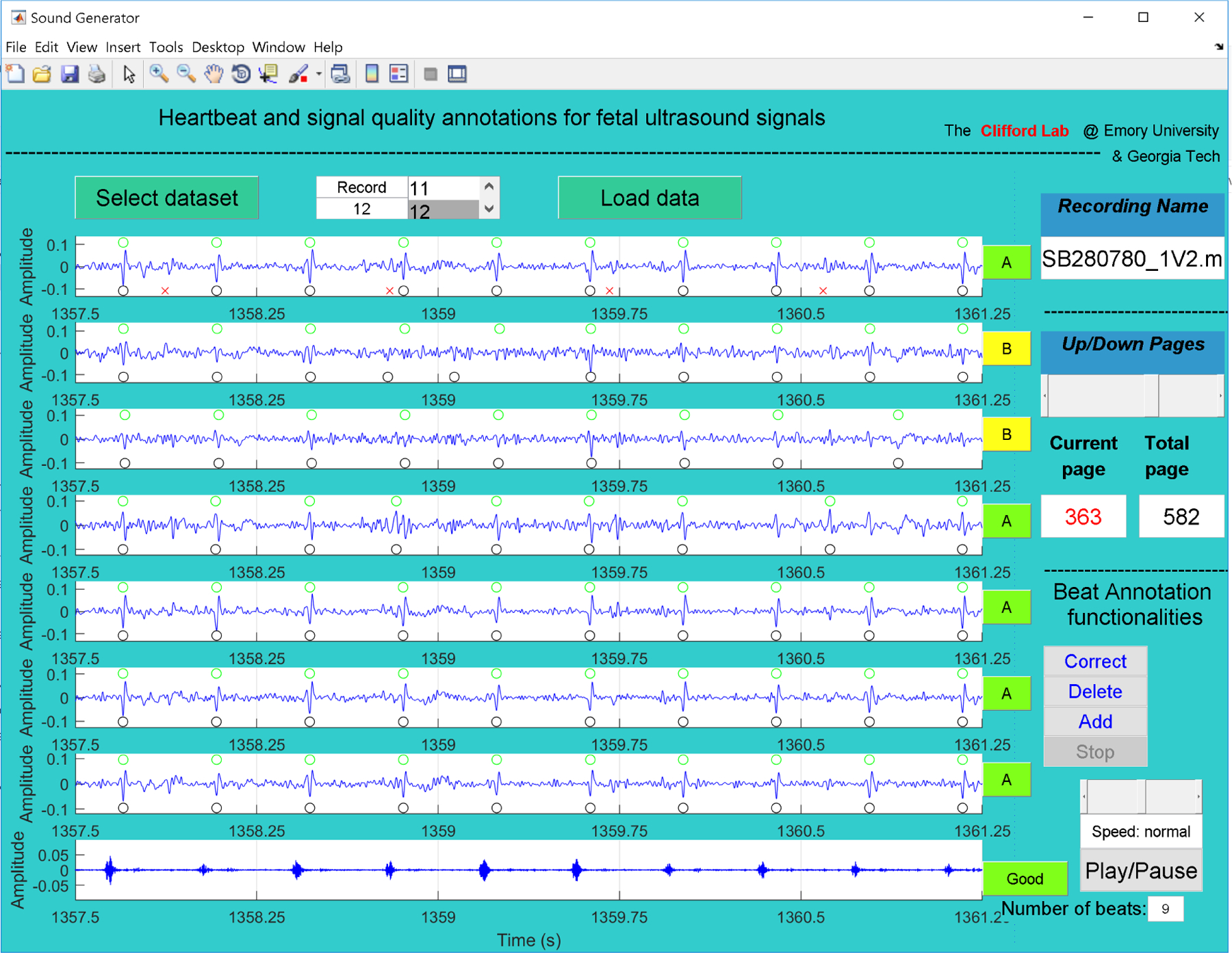
GUI used to annotate LUH database. The first seven channels correspond to abdominal fECG after filtering maternal components using an extended Kalman smoother and peak detection of fetal (black circles) and maternal beats (red crosses, upper plot) (Behar et al., 2014). The last channel in the plot is the 1D-DUS signal re-sampled at 4 kHz. Using buttons on the right of the GUI, and the automatic detection as a preliminary guide, two independent annotators provided quality of fECG and 1D-DUS. For good quality 1D-DUS, fECG beats are located (green circles in the upper part of each fECG subplot).

Two independent annotators used the Matlab GUI to assess the quality of 1D-DUS and fECG channels, and to place the beat time location based on fECG channels. For each 3.75 s segment, annotators listened to the ultrasound recording and noted the number of audible beats, and labeled the 1D-DUS quality using the same class hierarchy described in (Valderrama et al., 2018a), namely, good, poor, electrical interference, talking, silent, or unsure. Since 1D-DUS quality may affect the FHR estimation (Stroux, 2016), only 1D-DUS segments with good quality were retained for heart rate estimation. After labeling the 1D-DUS quality, annotators labeled each fECG channel as:

• A: All QRS complexes can be seen (although not necessarily in the same channel)

• B: Some QRS might be missing or some extra beats

• C: Lots of noise and absent signal/dropout but see at least two neighboring beats

• D: Almost completely noise

• E: Unsure

To annotate the beat time location, the visible peaks contained in the good quality fECG channels were used. As an initial estimate, the location provided by automatic fECG QRS detection was used; however, annotators were able to correct those locations using the GUI. To avoid confusing maternal breakthrough for fetal peaks, annotators used visual inspection of the maternal ECG and detected peaks, provided in the upper subplot of the GUI (red crosses in Figure 1), thus discarding any peak when it was aligned to a maternal peak and out of sequence. Observation across all fECG channels was used to improve the accuracy of beat time locations.

After finishing the annotation process for all the 1D-DUS and fECG channels and retaining segments with simultaneous high quality fECG and 1D-DUS, 5 of the 16 subjects were included, the remaining were eliminated due to high noise levels in either of the channels. (Data were collected serendipitously as part of another study in which 1D-DUS recording quality was not prioritized.)

To ensure that beat time locations were consistent, the difference in seconds, δ, of fECG peak times between the two annotators was compared. Figure 2 shows that for 95% of annotated beats, the difference between pairs of annotations was less than 50 ms. Therefore, a high level of trust was ensured in the fECG annotations.

Figure 2:

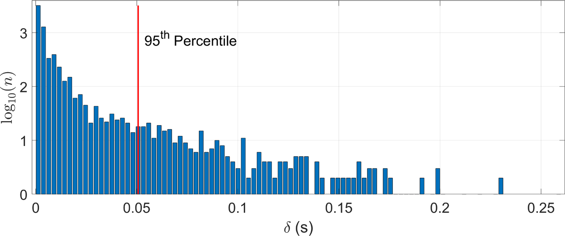
Histogram of time differences between beat time locations from two independent annotators. The horizontal axis, δ, is the difference in seconds of the two annotations for the fECG peak timing. The vertical axis represents a logarithmic scale of the count (n) of each difference. Note that 95% of the annotations differed by at most 0.05 s.

The reciprocal of the median of the interval between fECG peak times in a 3.75 s segment (scaled by 60) was used to estimate the reference FHR. The median is highly robust to missing or extra peaks (Clifford et al., 2006).

2.2.2. Annotation of Oxford JR Database

Each of the 1 minute-length 1D-DUS signals were labeled by three different expert annotators using a Matlab GUI. Each reviewer independently labeled the quality of each second as:

• Noise: No information available in the signal.

• Poor: The signal may contain heartbeats, but it is too ’noisy’ to identify them.

• Intermediate: Difficult to hear heartbeats, but can be done with some effort. Heart rhythm detection may be possible.

• Good: Some background noise, but heartbeats can be heard clearly. Heart rhythm detection is possible.

• Excellent: Almost no background noise, heartbeats are easy to identify, heart rhythm detection is possible.

These categories defined the signal quality of the 1D-DUS segments. Furthermore, while annotators were listening to the 1D-DUS segment, they clicked a mouse to indicate the temporal location of each beat that they heard.

After labeling all the segments, one-minute segments were split into 3.75 s with no overlap. Only segments in which at least two annotators labeled the same class were used. The manual FHR was estimated by first aligning the points that annotators clicked for the beat sound. The closer points were grouped and their median was taken as initial beat location. These locations were corrected using the homomorphic envelope of the 1D-DUS segment. Starting from the last beat location of the segment, the closest peak was searched in a window starting one interval prior to the annotation and ending 1/4 interval thereafter. Then, using reverse iteration, each peak time was corrected by finding the maximum peak in a window of ± 15 BPM from the last corrected peak. More description of the method can be found in (Stroux, 2016).

Similar to the LUH dataset, for the Oxford JR dataset, the manual FHR was estimated as FHR = 60/median(I) BPM, where I is a vector containing the difference in seconds between two corrected adjacent peaks.

2.2.3. Annotations of Guatemala RCT Database

For this dataset, only segments that had been manually classified as good quality in our earlier work (Valderrama et al., 2018a) were used. Since in Doppler ultrasound each cardiac cycle is represented by a combination of cardiac wall and valve movements (Shakespeare et al., 2001), it is extremely complicated to mark one specific point as a beat location, thereby producing a large variation among annotators. Listening to the data and attempting to hit a button when a beat is heard is also problematic since human reactions, keyboard delays, etc., add in large variable time delays (Stroux et al., 2016). To address this problem, we designed a Matlab GUI (Figure 3) to count the number of audible beats in each 3.75 s segment. The beat counting was performed by three independent annotators. The median number of beats over all three annotators, b, was used to define the FHR estimate as FHR = 60b/3.75 BPM.

Figure 3:

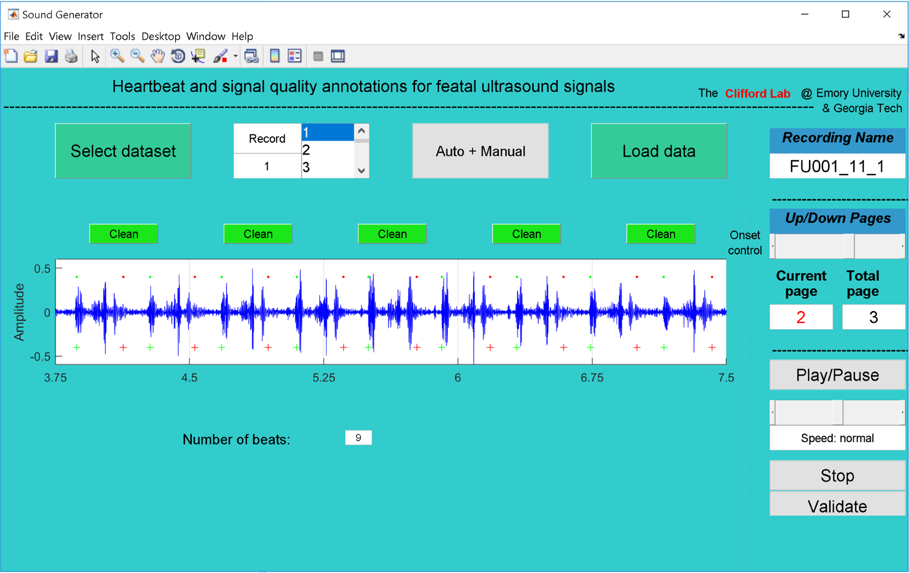
GUI used to manually annotate the number of beats in the Guatemala RCT dataset. Annotators listened to each 3.75 s segment, counting and recording the number of audible beats.

2.3. Datasets

The number of 1D-DUS segments obtained for each dataset after the manual FHR estimation process are displayed in Table 1.

Table 1:

Summary of final datasets used for developing fetal heart rate estimator. The Leipzig dataset was used for optimizing the parameters since it contains simultaneously recorded fECG, a validated reference technique used for fetal cardiac monitoring. The remaining two dataset were used as independent test sets. For the Oxford dataset, the number of good and excellent quality segments are shown in parenthesis.

Database	Number of subjects	Number of 3.75 s segment	GA range (weeks)	Additional recordings	Use
Leipzig (LUH)	5	721	20–27	fECG, maternal ECG	Training
Oxford JR	17	894 (482)	20–38	1D-DUS quality labels	Testing
Guatemala RCT	99	3938	20–40	blood pressure, maternal HR	Testing

Figure 4 shows the distribution of the manual FHR estimations of the three datasets used in this work. Note that they form very different distributions, having been derived from datasets with different gestational ages. The LUH dataset contained subjects with lower gestational ages (generally less than 27 weeks) than the Oxford and Guatemala RCT datasets and FHR is known to be higher earlier at earliers stages of pregnancy (Ibarra-Polo et al., 1972). Accordingly, the histogram of the Leipzig manual FHR estimations had a peak around 150 BPM, whereas the other two datasets had a peak around 135 BPM. Note also that the majority of FHR estimated values are found concentrated into in the 110 to 160 BPM normal interval (Pildner von Steinburg et al., 2013). The LUH and Oxford JR datasets appear to have continuous distributions since manual annotations were performed based on the timing of the peak. On the other hand, the Guatemala RCT dataset contained a much more pronounced quantization because the annotation of this dataset was based on the number of audible beats in a 3.75 s window, ranging between 112 to 192 BPM (7 to 12 beats in 3.75 s).

Figure 4:

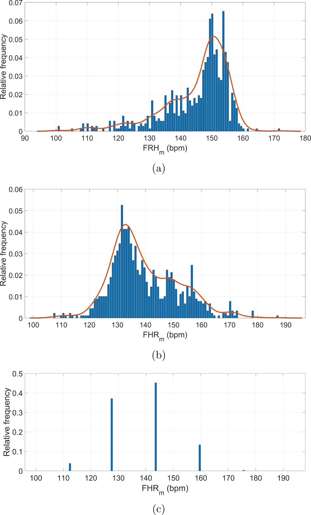
Manual FHR (FHR_m) estimations for datasets: (a) Leipzig dataset; (b) Oxford dataset; (c) Guatemala RCT dataset. The solid (red) lines represent the probability distributions smoothed using a normal kernel function (Bowman and Azzalini, 1997). The Leipzig and Oxford datasets appear to have continuous distributions, while the Guatemala RCT contained a much more pronounced quantization.

2.4. Heart rate estimator

The following subsections describe our AC-based method to estimate FHR from 1D-DUS signals. The corresponding source code is available from a public repository (Valderrama et al., 2018b) under a BSD Clause 2 license.

2.4.1. Noise removal

As extreme noise affects the estimator prediction, noise spikes were removed, using the algorithm presented in (Schmidt et al., 2010). This algorithm splits the 1D-DUS segment into windows of a specified interval. In this work, the interval was defined to be 0.75 s to contain at least one beat based on a heart rate of 80 BPM, which is the lower bound on a normality interval (Pildner von Steinburg et al., 2013). For each of the windows, the maximum absolute amplitude (MAA) was calculated. Then, windows whose MAA value was higher than a threshold, defined as three times the median MAA of the segments, were marked as containing spikes. To remove spikes, the marked window with the greatest MAA was selected, defining the spike interval as the first zero-crossing before and after the MAA. That interval was set to zero. After this, the median windows MAA and threshold were recalculated, and the procedure was repeated until there were not windows with MAA greater than the threshold.

2.4.2. Frequency range of interest

The cardiac frequency range for the device used here was estimated from observations in the current literature. For instance, Tutschek et al. (2003) found that from the 12th gestational week, the peak cardiac wall velocities could be measured by tissue Doppler echocardiography. This finding suggests that cardiac wall movement, in particular ventricular motion, may be present in any acquired 1D-DUS signal. According to the authors, the axial cardiac wall velocities of the right and left ventricle are described by the following second order data fitting models:

$$\begin{array}{l}{V}_{RV}=0.017x^2+0.5944x+9.0522,\hfill \\ V_{LV}=0.009x^2+0.2104x+5.0742,\hfill \end{array}$$ (1)

where V_RV and V_LV , in cm/s, are the axial cardiac wall velocities of the right and left ventricle, respectively; and x is the gestational age in weeks.

To define the cardiac frequency range, the empirical models of the cardiac wall velocities (Eq. 1) were combined with the equation of Doppler magnitude frequency shift f_D, defined as (Kohler and Sumner, 2014):

$$f_D=\frac{2f_o}{c}V\text{cos}\theta ,$$ (2)

where f_D is the measured change in frequency (Hz), f_o the frequency of emitted ultrasound transducer in Hz, c the speed of sound in soft tissue in m/s, V the velocity of the reflecting interface in m/s and θ is angle the between ultrasound beam and the surface in radians.

The hand-held Doppler ultrasound device used in this work has an f_o of 3.3 MHz. The speed of sound in human tissue (c) in standard-compliant ultrasound machines is 1540 (m/s) (Eik-Nes, 2009). The maximum f_D is achieved when θ is 0 rad, whereas it is minimum when θ is π/2 rad. Using a gestational range interval from 20 to 40 weeks, the maximum and minimum values for measured change in frequency (Hz) were estimated (see Table 2). Based on Table 2, the cardiac frequency range was extracted using a 25–600 Hz bandpass filter. Low frequencies (below 25 Hz) were removed to reduce disturbances introduced by fetal or device movement.

Table 2:

Expected minimum and maximum values for measured change in frequency (Hz) from over a gestational age ranging from 20 to 40 weeks. RV and LV stands for right and left ventricular, respectively.

Variables	RV	LV	RV	LV
GA [weeks]	20		40
V [m/s]	0.04	0.04	0.12	0.11
fDmin [Hz]	0	0	0	0
fDmax [Hz]	169.89	191.41	534.69	473.92

2.4.3. Homomorphic envelope

Given the capacity of complex homomorphic filtering to extract envelopes from physiological processes (Rezek and Roberts, 1998), such as electromyographic or respiratory signals, in this work we applied this method to the 1D-DUS segments. The rationale behind this technique is to assume that physiological processes are generated by a multiplicative system as:

$$s(t)=A_m(t)\text{ cos}\left(w_{c}t\right),$$ (3)

where A_m(t) is the modulating signal carrying the information, and cos(w_ct) is the carrier signal oscillating at a frequency of w_c. However, since the carrier frequency, w_c, is unknown, the demodulation is not straightforward. It can however, be achieved by transforming the modulation process into a system of linear filters. Although this transformation can be performed as:

$$\text{log}(s(t))=\text{log}\left(A_m(t)\right)+\text{log}\left(\text{cos}\left(w_{c}t\right)\right),$$ (4)

applying it directly to real signals can cause a major concern since logarithm has a singularity at zero. Nevertheless, this problem is alleviated by using the analytical signals as is presented in (Rezek and Roberts, 1998). Specifically, the Hilbert transform is used, which converts the real function, s(t), into an analytical function as:

$$z(t)=s(t)+i\tilde{s}(t),$$ (5)

where $\tilde{s}(t)$ is the Hilbert transform of s(t). The analytical function, z(t), has the advantage that its magnitude, |z(t)|, is equivalent to that of the message signal in the amplitude modulation process. Thus, the magnitude, |z(t)| , is decomposed into amplitude and oscillating components by using Eq. 4. Then, the amplitude components are kept by using a low-pass filter. Finally, taking the exponential of the low-pass filter output, the homomorphic envelope of s(t) is extracted.

2.4.4. Automatic Fetal Heart Rate Estimation

The FHR was estimated by applying the ACF to the homomorphic envelope of the 1D-DUS signal. The ACF was estimated in time-domain using a rectangular window from lag 0 to the length of the 1D-DUs segment (i.e. 3.75 × 4000 = 15000 samples). As described in Box et al. (2015), the k − th lag correlation, r_k, of a sequence y[n] was calculated as:

$$r_k=\frac{c_k}{c_0},$$ (6)

where c₀ is the sample variance of y[n], and c_k is:

$$c_k=\frac{1}{T}\sum _{i=0}^{T-k}(y[i]-\overline{y})(y[i+k]-\overline{y}),$$ (7)

where $\overline{y}$ is the mean of y[n], and T the length of y[n].

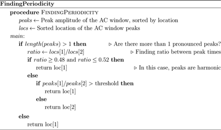
The envelope periodicity was determined from the ACF using the algorithm shown in Figure 5 and Appendix A. This algorithm found peaks within a window range of possible FHR values, which was defined by a lower interval value within 0.25–0.3 s (200–240 BPM) to an upper interval value within 0.8–1.0 s (60–75 BPM). Since the maximum window length using these values could be 0.75 s, the window may include at most two prominent peaks in the ACF.

Figure 5:

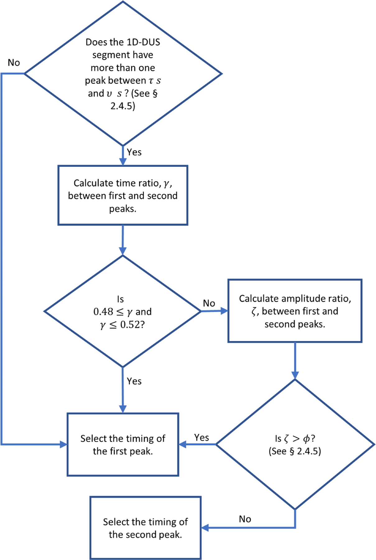
Flow diagram of algorithm used for finding the peak in the ACF to determine the heart rate period. Pseudocode for this flow diagram is provided in Appendix A.

If there are more than two pronounced peaks inside the search window, the algorithm performs additional steps to ensure that the peaks are not harmonics. Specifically, the ratio of their lag times, γ, are calculated. Since it is expected that harmonics are multiples of the fundamental frequency (Schwartz, 1968), the algorithm checks if γ is within the interval 0.5 ± 0.02. This interval was determined from the fact that three standard deviations of the 1D-DUS segments in the training data contained harmonics within this region. In case the peaks are harmonics, the temporal value (lag) of the first peak is selected as that which represents the periodicity. Otherwise, the first peak is selected only if the amplitude ratio between the peaks, ζ, is greater than a threshold, which was determined by parameter optimization described in the following section.

For instance, Figure 6 shows an example for one of the 1D-DUS segments. As can be seen, there are two peaks inside the search window. In this case, if the highest amplitude peak were selected without comparison to the lower amplitude peak, it would lead to an incorrect estimate of the heart rate period (i.e a period of 0.749 s or 80.1 BPM). The first peak correctly corresponds to a period of 0.382 s (157.3 BPM). The ratio of the peaks, γ, is 0.382/0.749, which is close to 0.5, indicating the second peak is a harmonic and should be ignored.

Figure 6:

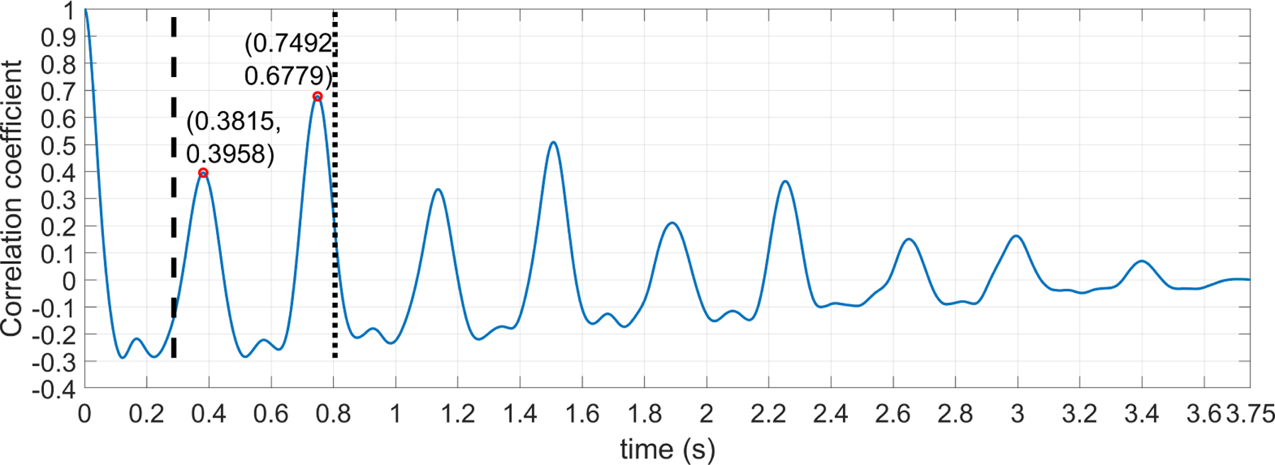
ACF for a 3.75 1D-DUS segment. Vertical dashed and dotted lines indicates the respective start and end points of the window within which a search is made for the peak related to the heart rate period. Peaks inside the window search are compared using algorithm showed in Figure 5 to find the right time location for the signal period.

Once the algorithm selects a peak time, the FHR of the 1D-DUS segment (i.e. periodicity) is determined as FHR = 60/l BPM, where l is the time location in second of the selected peak.

2.4.5. Parameter optimization

There are four parameters that must be optimized to estimate the FHR. The first is the cut-off frequency of the low-pass filter used to extract the envelope from the complex signal. The second (τ) and third (v) parameters are the lower and upper bounds of the interval of the window used for finding peaks in the autocorrelation. The fourth parameter, ϕ, is the threshold used for comparing the peaks amplitude within the search window.

The four FHR estimator parameters were determined using Bayesian optimization with 1000 iterations over the training set (a subset of the Leipzig dataset). The parameter search space was defined as shown in Table 3. The Bayesian optimization used the mean square error (MSE) of the difference between the manual FHR annotation and the FHR estimations of the training subjects (MSE_m–t) as the objective function to be optimized. In detail, given a parameter tuple within a search space bounds, the objective function first calculated the MSE_m–t of each training subject, and then averaged the individual MSE_m–t values.

Table 3:

Parameter intervals used in the Bayesian optimization process.

Parameter	Lower bound	Upper bound
Cut-off frequency (Hz)	2	15
Minimum Period (s)	0.25	0.3
Maximum Period (s)	0.8	1.0
Threshold	0.55	0.99

At the beginning, the Bayesian optimization algorithm defined a Gaussian process (GP) for the objective function with mean 0 and covariance kernel defined by the Automatic Relevance Determination (ARD) Matérn 5/2 kernel (Snoek et al., 2012). At each iteration, the GP was updated using the posterior probability of the new evaluated tuple. The tuple to evaluate at each iteration was selected using the expected-improvement acquisition function (EI) (Gelbart et al., 2014). This function selected the tuple that maximized the expected improvement on the objective function based on the associated GP. The parameter expectation ratio of the acquisition function was set to 0.5 to avoid being stuck at local maxima, thus giving the same weight to explore and exploit parameter tuples in the solution space. After the 1000 iterations, the parameter tuple with the minimum value of the objective function was selected as the parameters for the FHR estimator.

2.5. Performance assessment

Since the LHU dataset contained both 1D-DUS signals and simultaneous abdominal fECG, it provided the most accurate reference point from which to start. We trained our FHR estimator using 60% of this dataset so that the fECG annotations were used as the primary reference. The remaining 40% of the LHU dataset was used as validation to reduce the chances of model overfit. The trained model was then tested with the Oxford JR and the Guatemala RCT datasets to evaluate generalizability performance. It is important to note that these two datasets were excluded from the training procedure because these latter two datasets contained no fetal ECG as a reference and including all of the populations in the training data would lead to overfitting (Liu et al., 2016). This process is somewhat similar to that of the commercial device setting, in which algorithms are trained on relatively few recordings, but are expected to work on a large variety of populations.

2.5.1. Training process

The Leipzig dataset was stratified by subject into training and validation sets, ensuring that manual FHR values between the two groups did not differ significantly (p-value > 0.05, Wilcoxon rank sum test). Thus, the training set contained a total of 430 3.75 s segments from three subjects, while the validation set contained 291 segments of 3.75 s from the remaining two subjects.

After optimizing parameters on the 1D-DUS segments of the training subjects, the FHR estimator was tested on the segments of the validation subjects. As well as ensuring a good out of sample optimization, the validation set was also used to check that the method did not estimate the maternal heart rate (MHR) rather than FHR. To this end, the automatic FHR estimations were compared to the maternal heart rate to ensure that the method was indeed estimating the fetal cardiac cycle. (The MHR was calculated using the maternal ECG simultaneously recorded with the 1D-DUS signals).

2.5.2. Testing process

Using the optimal parameters obtained from the Leipzig dataset, the fetal heart rate estimator was tested on the Oxford and Guatemala RCT datasets separately to see if the algorithm generalized to multiple different populations. For both test datasets, the automatic FHR estimations were compared to those manually estimated by the annotators. To perform this comparison two methods were used. First, we defined a positive percentage of agreement (PPA) as a FHR estimation that are within 10% of a manual FHR. This bound was deviated from previous works, which have performed comparison to asses the equivalence in success rate, reliability and accuracy between FHR measurements obtained from ultrasound CTG and abdominal fetal ECG (Reinhard et al., 2013, 2010). This PPA has been also used to compare ultrasound CTG and abdominal fetal ECG fetal scalp ECG (Euliano et al., 2017; Cohen et al., 2012). Second, to show the bias and the level of agreement of our FHR estimator, Bland-Altman plots (Bland and Altman, 1986) were created.

In the Oxford dataset, FHR estimation was also calculated according to quality classes in the dataset. For the Guatemala RCT dataset, additional stratification by gestational age (GA) was performed to check if this variable was a confounder for FHR estimation. GA comparison was performed comparing all possible pairs of the available months (5 to 9 months). The significance level (α = 0.05) of the hypothesis test performed on the 10 possible pairs, $\left(\begin{array}{l}5\hfill \\ 2\hfill \end{array}\right)$, was corrected using the Bonferroni technique (α/10 = 0.005).

2.5.3. Comparison between Oxford JR and Guatemala RCT datasets

As datasets have different distributions (see Figure 4), we performed a two-sided Wilcoxon rank sum test to determine if the median of the errors between the Oxford JR and the Guatemala RCT datasets were significantly different. (A one sample Kolmogorov-Smirnov test was first applied to confirm that the error distributions were not normally distributed.) Only good quality 1D-DUS segments of both datasets were used so that meaningless comparisons between spurious estimates were not made. A total of 3934 and 479 segments for the Guatemala and Oxford datasets, respectively, were available for analysis.

3. Results

3.1. Optimized parameters and validation stage

Table 4 shows the best parameters obtained through the Bayesian optimization process. Window search was found to range between 0.29 s to 0.84 s, which was equivalent to 71.5 and 208.8 BPM, respectively.

Table 4:

Best tuple of parameters found by the Bayesian optimization process.

Cut-off frequency (Hz)	Minimum Period (s)	Maximum Period (s)	Threshold
14.8	0.287	0.839	0.650

Figures 7 and 8 show the performance of the trained FHR estimator on the validation set. As can been seen, 99% of the segments were within the PPA bounds, whereas the difference between the manual ($h_m^f$) and automatic FHR ($h_a^f$) was close to zero with a RSME of 3.68 BPM. The low bias suggests that optimized parameters were not overfitted, and therefore the resulting algorithm may be appropriate to other unseen data.

Figure 7:

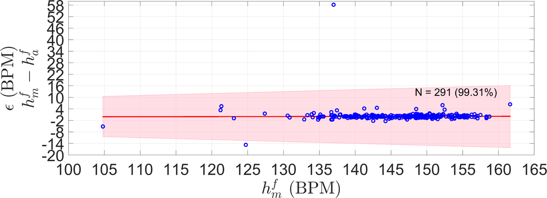
Error (ϵ) (difference) between manual FHR ($h_m^f$) and automatic FHR ($h_a^f$) of the LHU validation set. Shaded area shows the 10% PPA bounds (error no greater than 10 percent of the $h_m^f$). N stands for the number of segments in the validation set, and in parenthesis is the percentage of segment satisfying the PPA. The red line is the robust least square fit of ϵ along the manual FHR estimations ($ϵ=-0.571+0.04h_m^f;r^2=0.99$).

Figure 8:

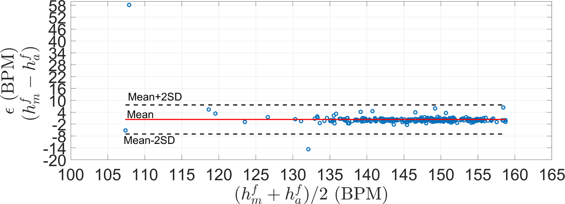
Bland-Altman plots for the LHU validation set. Mean (μ) and standard deviation (σ) of ϵ were 0.34 and 3.67 BPM, respectively. Limit of agreements (μ + 2σ) was [−7, 7.68] BPM. RSME was 3.68 BPM

In addition, to further evaluate the performance on the validation set, the automatic FHR was also compared to MHR (Figure 9). Only 1 out of 291 estimations was in the maternal range, thus suggesting that the 430 Doppler segments used for training the estimator indeed corresponded to fetal rather than maternal cardiac activity.

Figure 9:

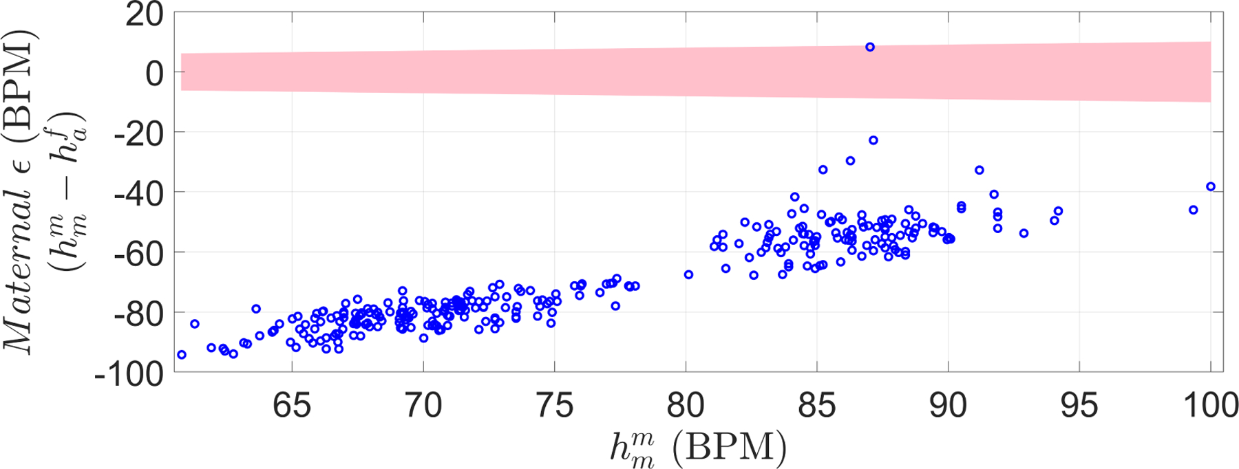
Maternal-Fetal difference in heart rate, for the validation set. This quantity was defined as the difference between maternal heart rate ($h_m^m$) and automatic FHR ($h_a^f$) estimation. The shaded area represents bounds in which automatic HR estimation is considered maternal instead of fetal based on the PPA ($h_a^f$ estimation within 10% of the recorded $h_m^m$). Only one estimation out of the 291 was within the shaded area, indicating a possible maternal recording (from maternal arteries).

3.2. Oxford dataset

Using the optimal parameters, the fetal heart rate estimator was applied to the 1D-DUS segments of the Oxford JR dataset, which included data of different quality levels. Figure 10 shows the difference between the manual FHR and the automatic FHR discriminated by quality class. For all the signal quality classes, the FHR estimation algorithm satisfied the PPA bounds over 87% of the time for data of intermediate or better quality.

Figure 10:

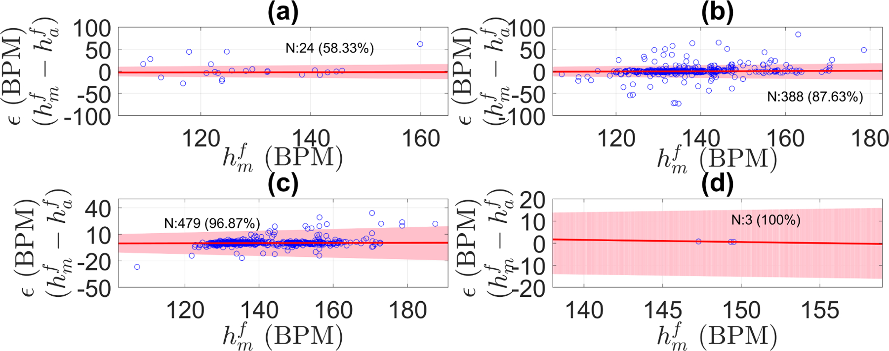
Error (ϵ) in fetal heart rate estimation discriminated by signal quality for the Oxford dataset: (a) poor quality, (b) intermediate quality, (c) good quality, (d) excellent quality. ϵ was defined as the difference between manual FHR ($h_m^f$) and automatic FHR ($h_a^f$) estimations. Shaded area shows the PPA error bounds (error no greater than 10 percent of the $h_m^f$). N stands for the number of segments in that signal quality class, and in parenthesis is the percentage of segment within the tolerance error bounds. The red line is the robust least square fit of ϵ along the manual FHR estimations (r² was 0.995, 0.997, 0.997, and 1.0 for poor, intermediate, good, and excellent quality, respectively).

Likewise, Table 5 shows the bias and variance of the difference between manual and automatic FHR estimations. As 1D-DUS quality increased, the bias and the variance decreased, thereby suggesting that signal quality category is critical for FHR estimation from 1D-DUS signals.

Table 5:

Mean and standard deviation, level of agreement, and RSME of the Bland-Altman analysis for the Oxford dataset discriminated by signal quality class.

Quality class	Mean (BPM)	Standard deviation (BPM)	Level of agreement (BPM)	RSME (BPM)
Poor	4.72	21.28	[−37.84, 47.28]	21.36
Intermediate	1.08	14.31	[−27.54, 29.69]	14.33
Good	0.52	4.62	[−8.72, 9.76]	4.65
Excellent	0.62	0.12	[0.38, 0.86]	0.63

3.3. Guatemala RCT dataset

Figure 12 shows the estimator performance for all the Guatemala RCT segments. As can be seen, 97% of the automatic FHR estimations fit the PPA bounds. Since the difference between two adjacent values of $h_m^f$ is 16 BPM, ϵ increased in 4.48 BPM (0.28×16) as $h_m^f$ goes from one available value to the next one.

Figure 12:

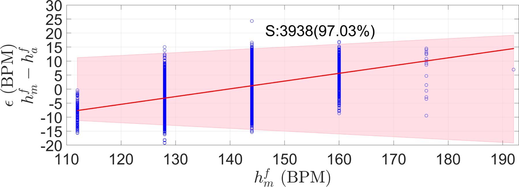
Error (ϵ) measured as the difference between manual ($h_m^f$) and automatic FHR ($h_a^f$) estimations for Guatemala RCT dataset. The shaded area represents the PPA bound, defined as no greater than 10 percent of the $h_m^f$. S stands for the number of segments, and in parenthesis is the percentage of segment satisfying the PPA bounds. Red line is the robust least square of ϵ along the manual FHR estimations ($ϵ=-38.63+0.28h_m^f;r^2=0.9962$).

Figure 13 shows a Bland-Altman analysis of the manual and automatic estimates of FHR in the Guatemalan RCT database. The mean difference between FHR estimates was close to zero, whereas the RSME was 6.64 BPM. The low bias and variance indicate that the FHR estimator can also achieve accurate estimations for datasets with a completely different distribution than that of the training set (see Figure 4).

Figure 13:

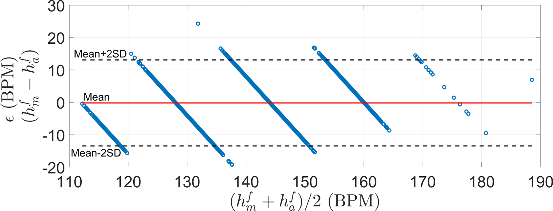
Bland-Altman plots for the Guatemala RCT dataset. Mean (μ) and standard deviation (σ) of ϵ were −0.17 and 6.63 BPM, respectively. Limit of agreements (μ + 2σ) was [−13.44, 13.10] BPM. RSME was 6.64 BPM

Figure 14 shows the results for the different GA found in the dataset. As can be observed, FHR estimation errors did not differ significantly statistically between gestational months (Bonferroni corrected p-value 0.005 (0.05/10); Wilcoxon rank sum test).

Figure 14:

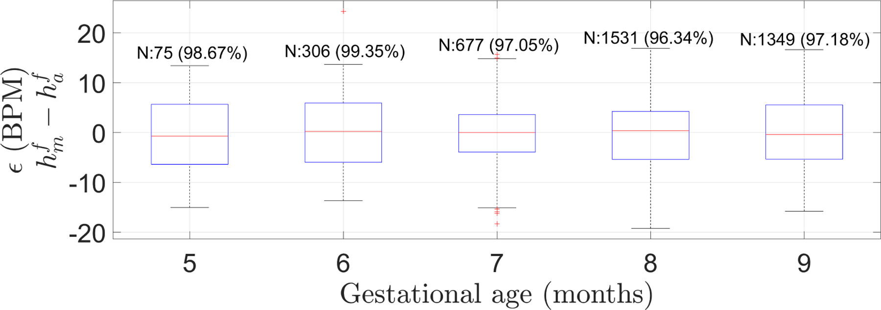
Box plot of the error (ϵ), defined as the difference between manual heart rate ($h_m^f$) and automatic FHR ($h_a^f$), for Guatemalan RCT dataset grouped by gestational age in months. N indicates the number of segments in the GA group and in parenthesis is the percentage of segments satisfying the PPA 10% error tolerance. FHR estimations did not statistically significantly differ among any possible pair of gestational months (Bonferroni corrected p-value of 0.005 (0.05/10); two-sided Wilcoxon rank sum test).

3.4. Comparison between Oxford JR and Guatemala RCT datasets

The medians of the distributions of the errors between $h_m^f$ and $h_a^f$ were not statistically significant (p=0.44; two-sided Wilcoxon rank sum test). Therefore, it seems that the distribution type did not affect the performance of the FHR estimator.

4. Discussion

4.1. Interpretations of Findings

The performance of the AC-based method presented here indicates that FHR can be reliably estimated from 1D-DUS signals, particularly when coupled with a signal quality metric. Specifically, our method were able to estimate FHR within 10% of the manual estimated FHR, achieving these estimations with a low bias and variance. It is notable that our method accurately estimates FHR using autocorrelation, which is an inexpensive technique requiring few computational steps and little memory, thus saving cost and execution time. Presented results suggest that our method is a simple option able to achieve comparable FHR values to those provided by fECG, which is considered a validated reference.

In comparison with previous methods which reported a correlation coefficient, r, of 0.977 (Peters et al., 2004), and 0.992 (Jezewski et al., 2011) between estimated FHR and fECG measurements, our presented AC-method obtained an r coefficient of 0.9226 and 0.8319 for the good quality segments of the two test datasets (Oxford and Guatemala RCT). Although our values were lower, it should be noted that the methods cannot be directly compared since they were not tested on the same dataset. In fact, the methodology used here to train and test the FHR estimator indicates that parameters found with Bayesian optimization seem to be generalizable to other datasets. In contrast, previous methods were tested with few patients (Jezewski et al., 2011) or with recordings of a single patient (Peters et al., 2004). Regarding the recently proposed EMD-Kurtosis method that claims to give more accurate estimations than standard AC-based methods (Al-Angari et al., 2017), our method did not optimize the parameters on data used for both training and testing, thus making generalizability much more likely.

Our AC-based method demonstrated its robustness to the acquisition environment. Although the Leipzig and Oxford datasets were recorded in hospital environments, performed by medical professionals, the method also achieved equivalently satisfactory results for the Guatemala RCT dataset, which was acquired in rural areas by non-medically trained users. Likewise, on the Guatemala dataset, the FHR estimator achieved similar results for pregnancies with GAs greater than 20 weeks (5 months), thus suggesting that gestational age is not a confounding variable for the estimator (and indicating its promise for future work on predicting GA and growth-related problems). Moreover, unlike previous research that used data at intrapartum stages and direct fECG for training there methods (Jezewski et al., 2008, 2011; Peters et al., 2004), here we showed that FHR estimation from 1D-DUS is also possible for antepartum stages. Finally, based on MHR comparisons performed for the validation set of the Leipzig dataset, it is evident that the method presented here estimates fetal heart rate using fetal cardiac activity rather than maternal one.

The optimized parameters trained over the 60% of the LHU subjects were able to extend to the other two datasets (Oxford JR and Guatemala RCT) regardless of the fact that their distributions of the fetal heart rates were different in the other datsets (see Figure 4). Indeed, there was no statistically significant difference estimations of FHR on the test datsets.

Although the AC-based method obtained accurate estimations for all tested datasets, it is important to note that since the Guatemala dataset is more quantized than the Oxford dataset, there is a larger quantization error for the former dataset. Indeed, since the difference between two possible reported values over 3.75 s windows was 16 BPM (Δ = 16), the method has a quantization error of ± 8 BPM (Δ/2=8), whereas the Oxford dataset did not have such as coarse quantization error.

4.2. Study Limitations

As previous research has reported, signal quality has been shown to be a relevant issue for heart rate estimation using AC-based methods (Stroux, 2016; Al-Angari et al., 2017). In fact, for the Oxford dataset, in which segments of different quality were available, the accuracy of the estimation depended on the 1D-DUS quality. This low accuracy for poor quality signals is explained by the fact that the ACF fails to provide a reliable determination of the signal periodicity when it contains additional spikes caused by noise. Nevertheless, the AC-based FHR estimation method presented here has been shown to be an accurate method across multiple datasets, mapping closely to industrial guidelines, for data of intermediate or better quality. We do not expect any system to provide good heart rate estimation when data are heavily corrupted, and in fact it is more important at that point to not report heart rate, but to report that the data are non-analyzable. In our earlier works, (Stroux and Clifford, 2014; Stroux, 2016; Valderrama et al., 2017, 2018a), we demonstrated accurate methods for separating low from good quality data, and even identifying the etiology of the noise. Therefore, coupling these works together may lead to a robust system that could be used in an automatic or semi-automatic manner.

Although all the datasets used here were acquired with the same hand-held device introduced in (Stroux, 2016; Stroux et al., 2016), all datasets were recorded and manually annotated by independent volunteers, thereby reducing or eliminating any dependency among them. Future work should evaluate the performance of the method presented here using 1D-DUS acquired with different devices; however, promising results obtained here suggest that the method would estimate suitable results with minimal adjustment. One of these adjustments could be the frequency ranges for filtering the cardiac wall velocities since the ultrasound frequency might be different for other devices, thus modifying values presented in Table 2.

One limitation of our implementation was the small number of simultaneously acquired Doppler and fECG recordings available for training. The dataset was collected by a partner group as an ancillary study to a larger study, and we had no control over it (Andreotti, 2016). As a consequence, the quality was variable, and some recordings were discarded as the quality of fECG was not high enough to manually identify fetal heartbeats. Nevertheless, the promising results obtained on the two independent datasets suggest the potential for the method introduced here to estimate FHR from 1D-DUS signals.

This study was not intended for assessment of FHR during labor and delivery, but rather for hand-held point of care devices. However, we also note that we see no theoretical reasons that the conclusions reached in this paper would not hold during labor and delivery outside of the period of contractions (where the data are well known to be very noisy).

Based on parameters shown at Table 4, the AC-based method introduced in this work could detect FHR values ranging from 71.5 to 208.8 BPM. The lower bound at 71.5 BPM could be a drawback for the detection of some bradycardia abnormalities, which are associated with lower FHR values. Nevertheless, the upper bound to detect bradycardia is different among the most common fetal monitoring guidelines (Santo et al., 2017). In particular, the International Federation of Gynecology and Obstetrics defines fetal bradycardia as a heart rate under 80 BPM, whereas the American College of Obstetricians and Gynecologists and the United Kingdom National Institute for Health and Care Excellence use 100 BPM and 110 BPM, respectively. Therefore, since our method is able to detect FHR estimations between 71.5 and 110, some bradycardia cases could be detected. We also note that the data used here is not relevant for labor, which is out of scope and not relevant to this research. For labor and delivery, the ECG has been shown to be superior (Sameni et al., 2009). We are specifically interested in tracking heart rate during the second and third trimesters before labor. Finally we note, that by definition, our data is representative of the patient population and encompasses the majority of heart rates we would encounter.

4.3. Future Directions

The rationale for the current research was to present a baseline for future FHR estimation methods. This serves several future directions of research and device design. For instance, the AC-based FHR estimation method presented in this work could help with the assessment of the accuracy of commercial Doppler transducers, which appear to use similar, but black-box AC-based methods. This work could improve the quality of regulatory submission and provide consumers with a more objective insight into the performance of a DUS FHR device. Furthermore, per (Stroux, 2016), the method described in this paper could serve as an auxiliary method for initializing more accurate FHR and FHR variability estimators.

5. Conclusion

This work presents a simple but promising method to estimate FHR from 1D-DUS signals acquired using a hand-held Doppler transducer, obtaining estimations within 10% of the reference FHR values. The presented method is generalizable, in contrast to other methods presented in literature, and robust to the recording environment and operator skill. Therefore, the described AC-based method is valuable in itself as an estimator of FHR in all sorts of applications, including outside of the controlled hospital environment. By ensuring accurate estimation of FHR, a basis for fetal cardiac monitoring is provided, establishing a basis from which future methods can be developed to estimate FHRV more accurately for assessing fetal wellbeing from 1D-DUS signals. We encourage benchmarked contributions to our source code, which is freely available from a public repository (Valderrama et al., 2018b) under a open source (BSD Clause 2) license.

Figure 11:

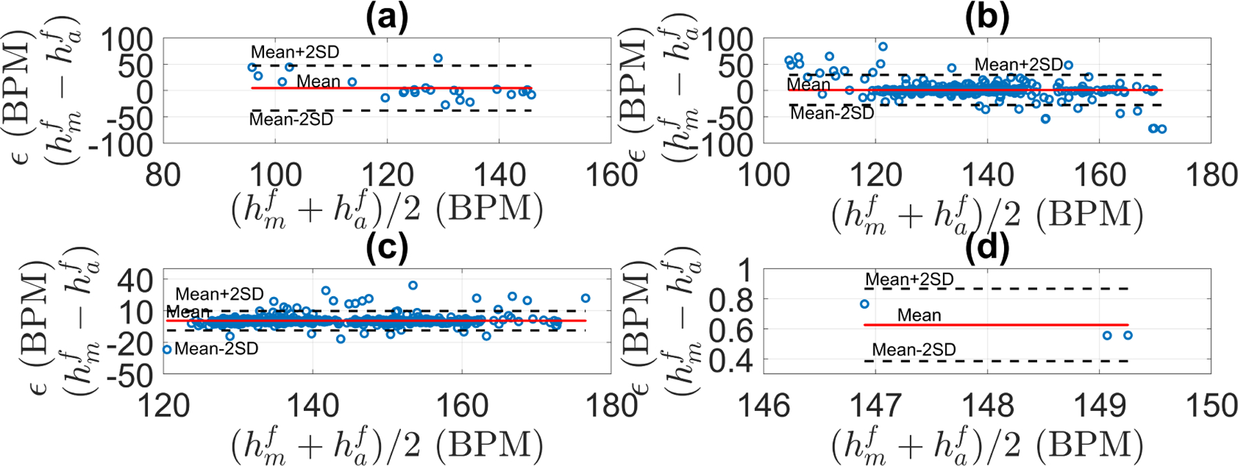
Bland-Altman plots for the fetal heart rate estimation discriminated by signal quality for the Oxford dataset: (a) poor quality, (b) intermediate quality, (c) good quality, (d) excellent quality. Mean and standard deviation, level of agreement, and RSME for each class are shown in Table 5.

Appendix A.

Algorithm for determining periodicity algorithm

References

- Al-Angari H, Kimura Y, Hadjileontiadis L, and Khandoker A (2017). A hybrid emd-kurtosis method for estimating fetal heart rate from continuous doppler signals. Frontiers in Physiology, 8:641. [DOI] [PMC free article] [PubMed] [Google Scholar]
- Andreotti F (2016). Extraction and detection of fetal electrocardiograms from abdominal recordings. PhD thesis, Technische Universitt Dresden. [Google Scholar]
- Behar J, Andreotti F, Zaunseder S, Li Q, Oster J, and Clifford GD (2014). An ecg model for simulating maternal-foetal activity mixtures on abdominal ecg recordings. Physiological Measurements, 35(8):1537–1550. [DOI] [PubMed] [Google Scholar]
- Bland JM and Altman DG (1986). Statistical methods for assessing agreement between two methods of clinical measurement. The Lancet, 327(8476):307–310. [PubMed] [Google Scholar]
- Bowman AW and Azzalini A (1997). Applied smoothing techniques for data analysis: the kernel approach with S-Plus illustrations, volume 18. OUP Oxford. [Google Scholar]
- Box G, Jenkins GM, Reinsel GC, and Ljung GM (2015). Time series analysis: forecasting and control. John Wiley & Sons. [Google Scholar]
- Cesarelli M, Romano M, and Bifulco P (2009). Comparison of short term variability indexes in cardiotocographic foetal monitoring. Computers in Biology and Medicine, 39(2):106–118. [DOI] [PubMed] [Google Scholar]
- Clifford GD, Azuaje F, and McSharry P (2006). Advanced methods and tools for ECG data analysis. Artech House Norwood. [Google Scholar]
- Cohen WR, Ommani S, Hassan S, Mirza FG, Solomon M, Brown R, Schifrin BS, Himsworth JM, and Hayes-Hill BR (2012). Accuracy and reliability of fetal heart rate monitoring using maternal abdominal surface electrodes. Acta Obstetricia et Gynecologica Scandinavica, 91(11):1306–1313. [DOI] [PubMed] [Google Scholar]
- Dawes G, Visser G, Goodman J, and Redman C (1981). Numerical analysis of the human fetal heart rate: the quality of ultrasound records. American Journal of Obstetrics and Gynecology, 141(1):43–52. [DOI] [PubMed] [Google Scholar]
- Eik-Nes SH (2009). Chapter 1 - physics and instrumentation. In Wladimiro JW and Eik-Nes SH, editors, Ultrasound in Obstetrics and Gynecology, pages 1 – 20. Elsevier, Edinburgh. [Google Scholar]
- Euliano TY, Darmanjian S, Nguyen MT, Busowski JD, Euliano N, and Gregg AR (2017). Monitoring fetal heart rate during labor: a comparison of three methods. Journal of Pregnancy, 2017. [DOI] [PMC free article] [PubMed] [Google Scholar]
- Gelbart MA, Snoek J, and Adams RP (2014). Bayesian optimization with unknown constraints. arXiv preprint arXiv:1403.5607 [Google Scholar]
- Hameed AB and Sklansky MS (2007). Pregnancy: maternal and fetal heart disease. Current Problems in Cardiology, 32(8):419–494. [DOI] [PubMed] [Google Scholar]
- Ibarra-Polo AA, Guiloff EF, and Gomez-Rogers C (1972). Fetal heart rate throughout pregnancy. American Journal of Obstetrics & Gynecology, 113(6):814–818. [DOI] [PubMed] [Google Scholar]
- Jezewski J, Kupka T, and Horoba K (2008). Extraction of fetal heart-rate signal as the time event series from evenly sampled data acquired using doppler ultrasound technique. IEEE Transactions on Biomedical Engineering, 55(2):805–810. [DOI] [PubMed] [Google Scholar]
- Jezewski J, Roj D, Wrobel J, and Horoba K (2011). A novel technique for fetal heart rate estimation from doppler ultrasound signal. Biomedical engineering online, 10(1):92. [DOI] [PMC free article] [PubMed] [Google Scholar]
- Jezewski J, Wrobel J, Matonia A, Horoba K, Martinek R, Kupka T, and Jezewski M (2017). Is abdominal fetal electrocardiography an alternative to doppler ultrasound for fhr variability evaluation? Frontiers in physiology, 8. [DOI] [PMC free article] [PubMed] [Google Scholar]
- Kohler TR and Sumner DS (2014). Vascular laboratory: Arterial physiologic assessment. In Cronenwett JL and Johnston KW, editors, Rutherford’s Vascular Surgery, chapter 15, pages 214–229. Elsevier Health Sciences, Philadelphia, PA. [Google Scholar]
- Lauersen NH, Hochberg HM, and George ME (1976). Evaluation of the accuracy of a new ultrasonic fetal heart rate monitor. American Journal of Obstetrics & Gynecology, 125(8):1125–1135. [DOI] [PubMed] [Google Scholar]
- Liu C, Springer D, Li Q, Moody B, Juan R, Chorro FJ, Castells F, Roig JM, Silva I, Johnson AE, Syed Z, Schmidt S, Papadaniil c., Hadjileontiadis L, Naseri H, Moukadem A, Dieterlen A, Brandt C, Tang H, Samieinasab M, R. SM, Sameni R, Mark R, and Clifford GD (2016). An open access database for the evaluation of heart sound algorithms. Physiological Measurement, 37(12):2181. [DOI] [PMC free article] [PubMed] [Google Scholar]
- Marzbanrad F, Stroux L, and Clifford GD (2018). Cardiotocography and beyond: a review of one-dimensional doppler ultrasound application in fetal monitoring. Physiological Measurement. [DOI] [PMC free article] [PubMed] [Google Scholar]
- Merz E (2004). Ultrasound in obstetrics and gynecology. Georg Thieme Verlag. [Google Scholar]
- Pardey J, Moulden M, and Redman CW (2002). A computer system for the numerical analysis of nonstress tests. American Journal of Obstetrics and Gynecology, 186(5):1095–1103. [DOI] [PubMed] [Google Scholar]
- Parer JT, Quilligan EJ, Boehm FH, Depp R, Devoe LD, Divon MY, Greene KR, Harvey CJ, Hauth JC, and Huddleston JF (1997). Electronic fetal heart rate monitoring: research guidelines for interpretation. American Journal of Obstetrics and Gynecology, 177(6):1385–1390. [PubMed] [Google Scholar]
- Peters C, ten Broeke E, Andriessen P, Vermeulen B, Berendsen R, Wijn P, and Oei S (2004). Beat-to-beat detection of fetal heart rate: Doppler ultrasound cardiotocography compared to direct ecg cardiotocography in time and frequency domain. Physiological measurement, 25(2):585. [DOI] [PubMed] [Google Scholar]
- Pildner von Steinburg S, Boulesteix A, Lederer C, Grunow S, Schiermeier S, Hatzmann W, Schneider KM, and Daumer M (2013). What is the normal fetal heart rate? PeerJ, 1:e82. [DOI] [PMC free article] [PubMed] [Google Scholar]
- Reinhard J, Hayes-Gill BR, Schiermeier S, Hatzmann H, Heinrich TM, and Louwen F (2013). Intrapartum heart rate ambiguity: a comparison of cardiotocogram and abdominal fetal electrocardiogram with maternal electrocardiogram. Gynecologic and Obstetric Investigation, 75(2):101–108. [DOI] [PubMed] [Google Scholar]
- Reinhard J, Hayes-Gill BR, Yi Q, Hatzmann H, and Schiermeier S (2010). Comparison of non-invasive fetal electrocardiogram to doppler cardiotocogram during the 1st stage of labor. Journal of Perinatal Medicine, 38(2):179–185. [DOI] [PubMed] [Google Scholar]
- Rezek I and Roberts SJ (1998). Envelope extraction via complex homomorphic filtering. Technical Report TR-98-9 Technical report. [Google Scholar]
- Roj D, Wróbel J, Horoba K, Przybyła T, and Kupka T (2010). Improving the periodicity measurement in fetal heart activity signal. Journal of Medical Informatics & Technologies, 16. [Google Scholar]
- Sameni R, Clifford G, Ward J, Robertson J, Pettigrew C, and Wolfberg A (2009). 664: Accuracy of fetal heart rate acquired from sensors on the maternal abdomen compared to a fetal scalp electrode. American Journal of Obstetrics & Gynecology, 201(6):S241. [Google Scholar]
- Sandmire HF and DeMott RK (1998). Electronic fetal heart rate monitoring: research guidelines for interpretation. American Journal of Obstetrics & Gynecology, 179(1):276–277. [DOI] [PubMed] [Google Scholar]
- Santo S, Ayres-de Campos D, Costa-Santos C, Schnettler W, Ugwumadu A, and Da Graça LM (2017). Agreement and accuracy using the figo, acog and nice cardiotocography interpretation guidelines. Acta obstetricia et gynecologica Scandinavica, 96(2):166–175. [DOI] [PubMed] [Google Scholar]
- Schmidt SE, Holst-Hansen C, Graff C, Toft E, and Struijk JJ (2010). Segmentation of heart sound recordings by a duration-dependent hidden markov model. Physiological measurement, 31(4):513. [DOI] [PubMed] [Google Scholar]
- Schwartz MF (1968). The acoustics of normal and nasal vowel production. The Cleft Palate Journal, 5(2):125–140. [PubMed] [Google Scholar]
- Shakespeare S, Crowe J, Hayes-Gill B, Bhogal K, and James D (2001). The information content of Doppler ultrasound signals from the fetal heart. Medical and Biological Engineering and Computing, 39(6):619–626. [DOI] [PubMed] [Google Scholar]
- Snoek J, Larochelle H, and Adams RP (2012). Practical bayesian optimization of machine learning algorithms. In Advances in neural information processing systems, pages 2951–2959. [Google Scholar]
- Stroux L (2016). A perinatal monitoring system for low-resource settings. PhD thesis, University of Oxford. [Google Scholar]
- Stroux L and Clifford GD (2014). The importance of biomedical signal quality classification for successful mHealth implementation. In 2014 Tech4Dev International Conference UNESCO Chair in Technologies for Development: What is Essential? EPFL, Lausanne, Switzerland. [Google Scholar]
- Stroux L, Martinez B, Coyote E, King N, Hall-Clifford R, Rohloff P, and Clifford GD (2016). An mhealth monitoring system for traditional birth attendantled antenatal risk assessment in rural guatemala. Journal of medical engineering & technology, 40(7–8):356–371. [DOI] [PMC free article] [PubMed] [Google Scholar]
- Tutschek B, Zimmermann T, Buck T, and Bender H (2003). Fetal tissue doppler echocardiography: detection rates of cardiac structures and quantitative assessment of the fetal heart. Ultrasound in obstetrics & gynecology, 21(1):26–32. [DOI] [PubMed] [Google Scholar]
- Valderrama CE, Marzbanrad F, Stroux L, and Clifford GD (2017). Template-based quality assessment of the doppler ultrasound signal for fetal monitoring. Frontiers in physiology, 8. [DOI] [PMC free article] [PubMed] [Google Scholar]
- Valderrama CE, Marzbanrad F, Stroux L, Martinez B, Hall-Clifford R, Liu C, Katebi N, Rohloff P, and Clifford GD (2018a). Improving the quality of point of care diagnostics with real-time machine learning in low literacy lmic settings. In ACM SIGCAS Conference on Computing and Sustainable Societies (COMPASS 2018). [Google Scholar]
- Valderrama CE, Stroux L, Springer D, and Clifford GD (2018b). Open source code for fetal heart estimator from one-dimensional doppler ultrasound signals. 10.5281/zenodo.1487995. [DOI] [Google Scholar]