A Deep Learning–based Model for Detecting Abnormalities on Brain MR Images for Triaging: Preliminary Results from a Multisite Experience

Abstract

Purpose

To develop a deep learning model for detecting brain abnormalities on MR images.

Materials and Methods

In this retrospective study, a deep learning approach using T2-weighted fluid-attenuated inversion recovery images was developed to classify brain MRI findings as “likely normal” or “likely abnormal.” A convolutional neural network model was trained on a large, heterogeneous dataset collected from two different continents and covering a broad panel of pathologic conditions, including neoplasms, hemorrhages, infarcts, and others. Three datasets were used. Dataset A consisted of 2839 patients, dataset B consisted of 6442 patients, and dataset C consisted of 1489 patients and was only used for testing. Datasets A and B were split into training, validation, and test sets. A total of three models were trained: model A (using only dataset A), model B (using only dataset B), and model A + B (using training datasets from A and B). All three models were tested on subsets from dataset A, dataset B, and dataset C separately. The evaluation was performed by using annotations based on the images, as well as labels based on the radiology reports.

Results

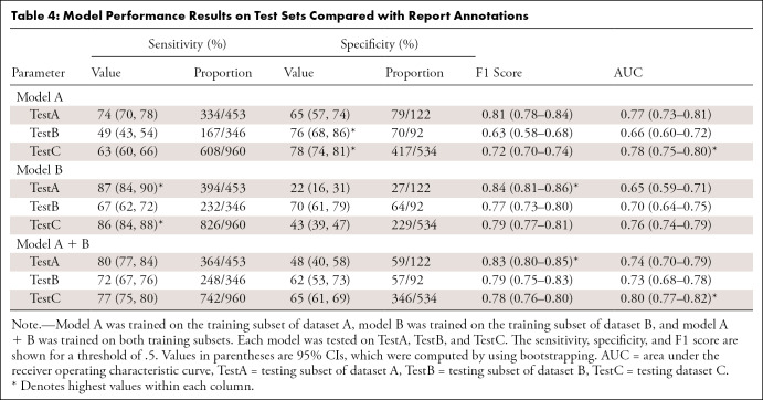
Model A trained on dataset A from one institution and tested on dataset C from another institution reached an F1 score of 0.72 (95% CI: 0.70, 0.74) and an area under the receiver operating characteristic curve of 0.78 (95% CI: 0.75, 0.80) when compared with findings from the radiology reports.

Conclusion

The model shows relatively good performance for differentiating between likely normal and likely abnormal brain examination findings by using data from different institutions.

Keywords: MR-Imaging, Head/Neck, Computer Applications-General (Informatics), Convolutional Neural Network (CNN), Deep Learning Algorithms, Machine Learning Algorithms

© RSNA, 2021

Supplemental material is available for this article.

Summary

A deep learning model to differentiate between normal and likely abnormal brain MRI findings was developed and evaluated by using three large datasets.

Key Points

• ■ A convolutional neural network was trained and validated on a large (>9000 studies) heterogeneous clinical dataset of fluid-attenuated inversion recovery brain MR images for the detection of abnormalities.

• ■ The performance reached an F1 score of 0.72 (95% CI: 0.70, 0.74) and an area under the receiver operating characteristic curve of 0.78 (95% CI: 0.75, 0.80) when tested on an independent dataset acquired from a different time period and different institution than the training set, thus showing the generalization capacity of the model and potential use for triaging purposes.

Introduction

MRI is increasingly used clinically for the detection and diagnosis of abnormalities (1). The resulting image overload presents an urgent need for an improved radiology workflow (2). Picture archiving and communication system worklist generation rules rely predominately on basic scan and demographic information (eg, acquisition time, modality, body part, referring medical service) found in the Digital Imaging and Communications in Medicine header (3). Because worklists cannot be sorted by imaging findings, examinations performed for diverse clinical reasons with varied types and severities of abnormalities are usually added to the same worklist and interpreted by radiologists in chronological order. Automatically identifying abnormal findings in medical images could improve the way worklists are prioritized, enabling improved patient care and accelerated patient discharge (4). Such automation has been shown to substantially improve turnaround time for the identification of abnormalities on head CT images (5) and chest radiographs (6).

Examples in the literature document automated diagnosis of specific conditions, such as brain tumors (7) and Alzheimer disease (8–11). A few limited approaches were developed for detecting brain abnormalities on the basis of imaging findings by using classic image analyses (12–15). In each of these experiments, datasets were derived from the publicly available website The Whole Brain Atlas (16), which includes only one sample patient for each brain abnormality consisting of no more than a few hundred image sections. The high accuracy reported is difficult to interpret given the limited dataset size, potentially resulting in model overfitting.

In this work, we describe the development and validation of a triaging system for brain MR images capable of detecting multiple abnormalities from three-dimensional volumetric images through use of a convolutional neural network (CNN). Because of the high diversity of patterns related to image abnormalities, classic machine learning approaches requiring feature engineering would be challenging to implement, whereas the use of CNNs allows the model to directly learn from the data the appropriate imaging features representing abnormalities. Our solution uses axial fluid-attenuated inversion recovery (FLAIR) sequence volumes as input, leveraging its high sensitivity for the identification of many brain abnormalities. The presented algorithm was developed and validated by using three large datasets collected from two different institutions on different continents. We report cross-site performance and demonstrate that additional clinical information from the radiology reports improved model performance.

Materials and Methods

Patient Datasets

This Health Insurance Portability and Accountability Act–compliant, institutional review board–approved study had patient consent waived. The data cohort consisted of three datasets of brain MRI studies acquired retrospectively from two different institutions located on different continents. Dataset A studies were collected from an inpatient site, whereas studies for datasets B and C were collected from multiple, predominantly outpatient sites from another institution. Datasets A (2007–2017) and B (2017) were originally collected for exploratory purposes. Dataset C (2019) contains consecutive studies collected after model development and is used only for model testing and clinical validation. Below are specific details for inclusion and exclusion for each of the datasets.

Dataset A.— This dataset included only studies acquired by using an axial FLAIR sequence (see Appendix E1 [supplement]), and children were excluded.

Dataset B.— This dataset included only studies acquired by using an axial FLAIR sequence (see Appendix E1 [supplement]); children were included, girls only (retrospective data that had been acquired independently for another study).

Dataset C.— This dataset included only studies acquired by using an axial FLAIR sequence (see Appendix E1 [supplement]), and children were included.

No studies were excluded on the basis of image quality, so as to reflect the heterogeneity of studies seen in routine clinical practice.

The resulting datasets A, B, and C consisted of 2839, 6442, and 1489 MRI brain studies, respectively. Data were de-identified by using the gdcmanon tool (http://gdcm.sourceforge.net/html/gdcmanon.html).

MR Image Acquisition

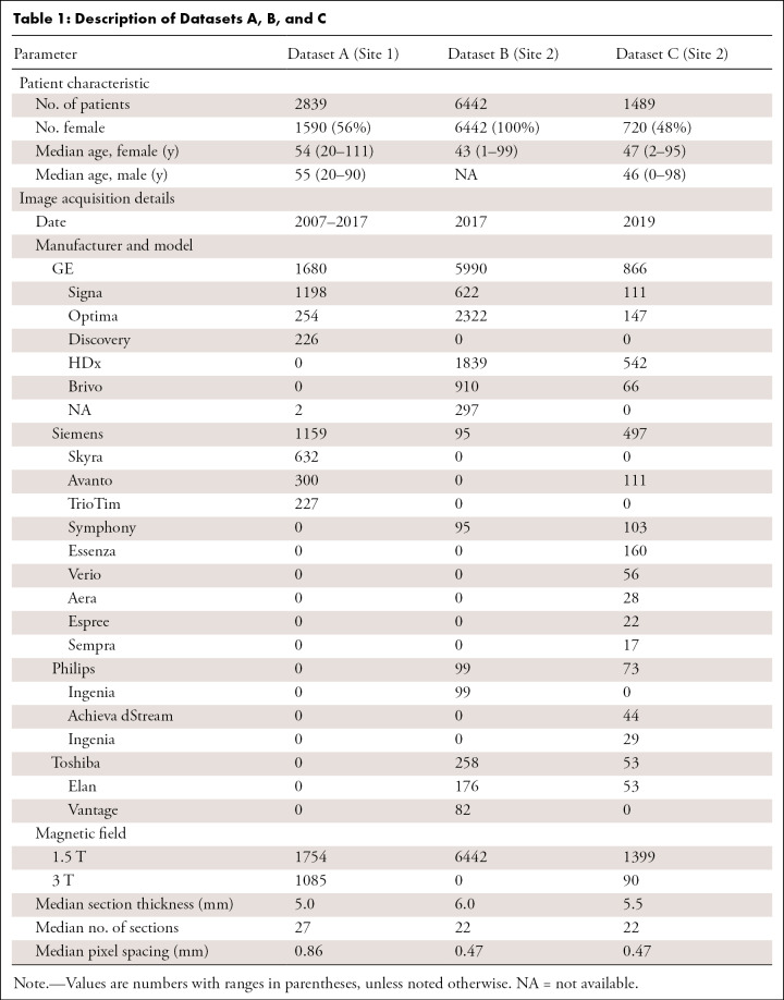
Dataset A images were acquired on General Electric and Siemens scanners, whereas datasets B and C images were acquired on General Electric, Siemens, Toshiba, and Philips scanners. Further MR image acquisition details are shown in Table 1.

Table 1:

Description of Datasets A, B, and C

Training, Validation, and Test Datasets

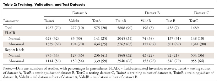
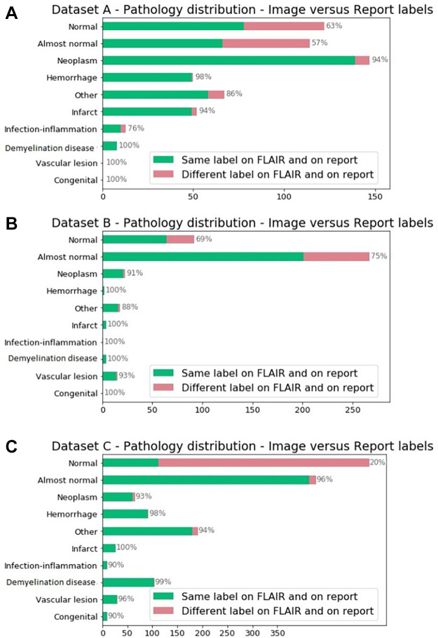
Dataset A was randomly split into training (70%, named TrainA), validation (10%), and test (20%, named TestA) sets. Dataset B was similarly split randomly into training (90%, named TrainB), validation (3%, named ValidB), and testing (7%, named TestB) subsets, which were then modified to achieve approximately the same number of positive samples in the validation and test sets as in dataset A for fair comparison while maximizing the number of training samples. Then 100% of dataset C was used as a test set only (TestC). The dataset breakdown allowed us to cover greater than 90% of abnormalities (Appendix E1 [supplement]). Axial FLAIR sequences were selected automatically (17). Tables 1 and 2 show dataset splits and acquisition, patient, and annotations details, highlighting the dataset heterogeneity. Figure 1 shows examples of dataset variability. Figure 2 shows pathologic finding distributions for each of the three datasets.

Table 2:

Training, Validation, and Test Datasets

Figure 1:

Examples of axial fluid-attenuated inversion recovery sequence acquisitions from studies within dataset A. From left to right: a patient with “likely normal” brain findings, a patient presenting with an intraparenchymal hemorrhage within the right temporal lobe, a patient presenting with an acute infarct of the inferior division of the right middle cerebral artery, and a patient with known neurocysticercosis presenting with a rounded cystic lesion in the left middle frontal gyrus.

Figure 2:

Pathologic distribution on (A) dataset A, (B) dataset B, and (C) dataset C identified by using annotations from the report. Reported in green are the percentage of annotations in which labels derived from the fluid-attenuated inversion recovery (FLAIR) MR image alone matched the report labels. Note on imaging that “almost normal” and other pathologic conditions are classified as “likely abnormal.”

Dataset Labeling

All studies were annotated by four radiologists, each with more than 5 years of experience reading brain MR images (F.C.K., B.C.B., O.L.J., F.B.C.M.). Annotations were performed at two different levels. First, radiology reports were used to label studies with 10 different categories: likely normal, almost normal (subtle benign findings such as small vessel disease), neoplasm, hemorrhage, infarct, infection or inflammatory disease, demyelination disease, vascular lesion, congenital, and “other” (for any finding that did not match the aforementioned categories). Next, FLAIR sequence acquisitions were reviewed by using the MD.ai (http://md.ai) annotation tool and categorized as presenting likely normal (label: 0) or likely abnormal (label: 1) findings. Data labels were subsequently rereviewed by a radiologist (F.C.K., O.L.J., and S.F.F. for dataset A; B.C.B. and F.B.C.M. for dataset B) from the distant institution to mitigate potential for institutional bias (eg, radiologist from site A reviews initial labels of radiologist from site B and vice versa). Labeling conflicts were adjudicated among the radiologists from each site with the final label defined by consensus.

For all datasets, radiologists were uniformly instructed to label examination findings as likely abnormal even if only subtle and/or benign-looking findings were present. For example, the presence of periventricular small white matter hyperintensities suggesting chronic small vessel disease constituted a reason to label the examination finding as likely abnormal. This type of finding is frequently seen in aging populations and is often considered as expected for certain age groups, whereas it could raise suspicions in a younger population. For a triage system, we chose to err on the side of over- rather than underlabeling these findings as likely abnormal.

Figure 2 shows the distribution of radiology report labels compared with those assigned by review of the FLAIR images alone. A large number of brain studies labeled as normal according to the reports were labeled as abnormal when reviewing the FLAIR images without the report, likely due to our labeling criteria designed to screen for abnormality. These figures also highlight the pathologic condition distribution differences among the datasets.

Machine Learning

The FLAIR axial series were downsampled to 256 × 256 × 16 voxels. Pixel intensities were normalized between 0 and 1 after clipping the 1% highest intensities. Data augmentation (translation, rotation, and Gaussian noise addition) was used.

A CNN architecture was implemented by using the TensorFlow library (18) to output a prediction between 0 (normal) and 1 (abnormal). The architecture consisted of five blocks of the following successive operations repeated twice: 3 × 3 × 3 convolutions, batch normalization, and leaky rectified linear unit activation followed by a max-pooling operation of size [2 2 1] (except for the final block, which had a max-pooling operation of size [2 2 4]). Those blocks had channel sizes of [24 32 46 64 72 80] and were followed by a dense layer of size 512 with a sigmoid activation function. The network was trained by using Adam optimization (19). The cross-entropy loss was minimized by using class weights of 0.7 for class 0 and 0.3 for class 1 to account for dataset imbalance. An L2 norm with weight of 10⁻⁴ was used as regularization for the convolution kernel weights. The batch sample size was set to 16. The same architecture was trained from random initialization for 125 000 iterations on the three different training sets (TrainA, TrainB, and TrainA + TrainB). For each set, 12 models were trained with different learning rates between 1e⁻⁵ and 1e⁻⁴ and a dropout rate of either 0.2 or 0.4 applied after the final dense layer.

Statistical Analysis

Model performance metrics included sensitivity, specificity, the F1 score, and the area under the receiver operating characteristic curve (AUC). For each metric, CIs are provided. The Python packages NumPy and SciPy were used for analysis. The CIs were computed through a percentile bootstrap approach by using uniform random selection with replacement and 5000 iterations (which provided regular histograms).

Performance on the validation sets was used to select the model with the highest performance for each dataset (named model A, model B, and model A + B to correspond with the training set on which each model was trained).

Results

Patient Dataset Overview

Models A, B, and A + B were each evaluated on the test sets of dataset A (TestA), B (TestB), and C (TestC, which was used only for testing). The different test sets contained 575 (TestA: 20% of dataset A), 438 (TestB: 7% of dataset B), and 1489 (TestC) brain MRI studies. Demographics are summarized in Table 1 and show important differences among the datasets. Dataset splits are shown in Table 2. In addition, Figure 2 and Table 1 show that pathologic conditions have differing prevalence across patient ages and inpatient versus outpatient care settings.

Comparison with FLAIR Labels

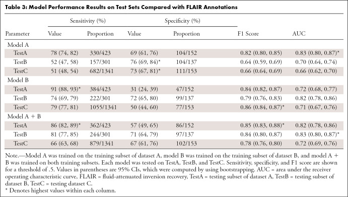
The performance metrics of model A tested on TestA and model B tested on TestB were similar (sensitivity, 78% [95% CI: 74, 82] and 74% [95% CI: 69, 79]; specificity, 67% [95% CI: 61, 76] and 72% [95% CI: 65, 80]; and F1 score, 0.82 [95% CI: 0.80, 0.85] and 0.79 [95% CI: 0.76, 0.83], respectively). CIs for these metrics largely overlap (Table 3). The AUC for model A tested on TestA was 0.83 (95% CI: 0.80, 0.87), and the AUC for model B tested on TestB was 0.82 (95% CI: 0.78, 0.86).

Table 3:

Model Performance Results on Test Sets Compared with FLAIR Annotations

When testing model A on TestB and model B on TestA, different trends were observed. Model A tested on TestB showed higher specificity (76% [104 of 137]) and a lower sensitivity (52% [157 of 301]). The F1 score was also lower at 0.64. For model B tested on TestA, the sensitivity was higher (91% [384 of 423]); however, the specificity was lower (31% [47 of 152]), which led to a higher F1 score (0.84). The AUC results were, however, in a similar range, with the AUCs being 0.70 (95% CI: 0.64, 0.74) for model A tested on TestB and 0.72 (95% CI: 0.68, 0.77) for model B tested on TestA. When tested on the opposite test sets, model A had a higher sensitivity than model B (91% [95% CI: 88, 93] vs 52% [95% CI: 47, 58]).

Not surprisingly, training on the combined training sets from datasets A and B (TrainA + TrainB) yielded good results on both TestA and TestB. Performance was comparable for the AUCs and F1 scores on the experiments in which the training and test sets were derived from the same dataset (ie, model A trained on TrainA and tested on TestA). The sensitivity of model A + B was higher on TestA than on TestB (86% [95% CI: 82, 89] and 81% [95% CI: 77, 85], respectively), and the opposite trend was observed for the specificity (57% [95% CI: 49, 65] and 71% [95% CI: 64, 79], respectively).

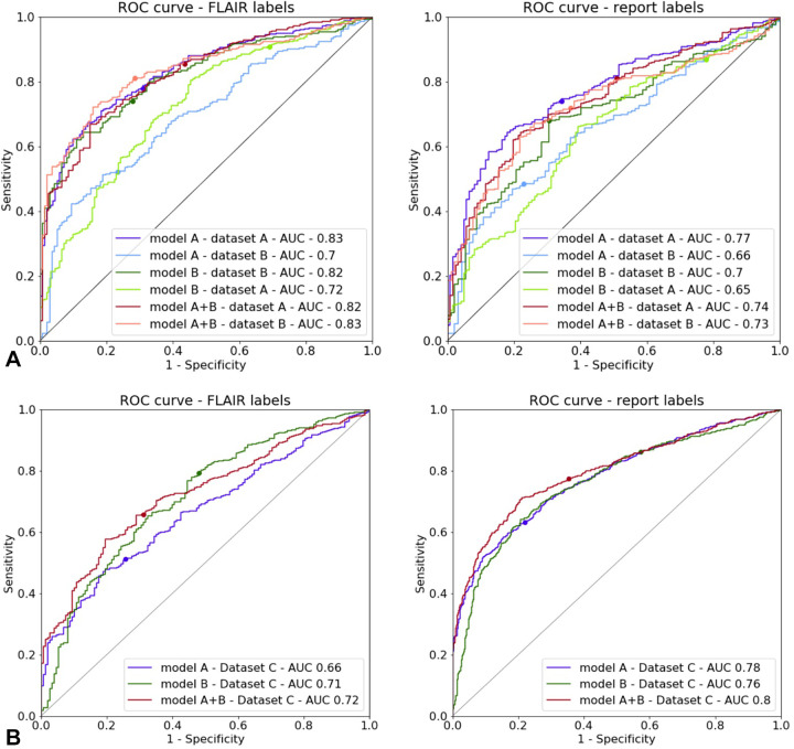
For dataset C, the performance of model A on TestC was lower than that of model A + B (AUC, 0.66 [95% CI: 0.62, 0.70] vs 0.72 [95% CI: 0.69, 0.76]). Model B produced similar AUC values when tested on TestC and TestA (0.71 [95% CI: 0.67, 0.76] and 0.72 [95% CI: 0.68, 0.77]). The highest performance was achieved by model A + B.

Comparison with Report Labels

The model performances were lower when using report labels from TestA and TestB (Table 4, Fig 3) than when using FLAIR labels. For instance, on TestA, the AUC of model A is lower on the report labels (AUC, 0.83 [95% CI: 0.80, 0.87]) than on the FLAIR labels (AUC, 0.77 [95% CI: 0.73, 0.81]). The highest performances on TestC were between an AUC of 0.76 (95% CI: 0.74, 0.99; model B) and an AUC of 0.80 (95% CI: 0.77, 0.82; model A + B), and the performance was higher when using report labels than when using FLAIR annotations. The analysis of pathologic condition distributions shows a lower discrepancy between the FLAIR and report labels on TestC than that between TestA and TestB (Fig 2). These results validate the choice of using the single FLAIR sequence for brain abnormality detection.

Table 4:

Model Performance Results on Test Sets Compared with Report Annotations

Figure 3:

Receiver operating characteristic (ROC) curves for models A, B, and A + B on (A) the testing subset of dataset A and the testing subset of dataset B, as well as on (B) the testing dataset C. Annotation labels from fluid-attenuated inversion recovery (FLAIR) (left) and radiology report annotation labels (right) were used as ground truths. The dots show the values corresponding to a threshold of .5. AUC = area under the ROC.

Discussion

Our experiments reveal reasonable performance for triaging purposes of a neural network for classification of likely normal or abnormal brain MR images acquired by using axial FLAIR sequences. Using a light CNN architecture yielded F1 scores and AUC metrics above 0.80. Such a system could enable the creation of a worklist of likely abnormal findings that could be used to improve radiology workflow. More experienced radiologists and neuroradiologists could focus on the likely most urgent or time-consuming studies. Trainees or junior attending physicians could use these finding-prioritized worklists as a learning opportunity. The potential decrease in reporting turnaround time and increased overall workflow efficiency were the goals of developing this artificial intelligence–enhanced optimization tool.

Analysis of our results provides the basis for additional investigations into potential performance improvements that would be achieved by using multiple, differing approaches, such as adding further MRI sequences (eg, diffusion-weighted sequences), improving input data normalization, increasing the complexity of the neural network architecture, and using larger and more diverse datasets for training and testing. Our results also highlight the lack of generalization that such models can exhibit. Our symmetrical experiments using different test sets derived from the datasets A, B, and C demonstrate a substantial decrease in model performance when using test sets collected from institutions different from those that collected the training data.

The challenge of multisite generalization of medical imaging computational approaches is not new (20) and is still a current issue. This is a difficult problem due to multiple confounding factors, including variability across patients, scanners, scanner operators, and disease prevalence in different populations (21). The large variability in the composition of brain MRI studies within and between institutions is a known issue, largely arising from different protocols, scanner models, and software and imaging artifacts. Research is ongoing to better harmonize data across scanners (22). However, even advanced data normalization processing may not be sufficient (23). In the presence of such a diversity of confounding factors, understanding and accounting for dataset shift errors is not straightforward (24).

In our experiments, having access to the radiology reports and patient demographic information helped elucidate some reasons for the shift. Reviewing dataset descriptions in Table 2 shows a similar normal versus abnormal imbalance across datasets. Differences in image acquisition parameters highlight potential explanations for these dataset shift errors. Dataset A included studies acquired retrospectively over a 10-year period, which were subject to image quality changes due to MRI scanner technology and imaging protocol evolution. This cohort includes balanced data acquired from two device manufacturers (Siemens and General Electric). Dataset B included studies consecutively acquired over a 1-year period with scanners from four different manufacturers (General Electric, Siemens, Toshiba, and Philips) and presented higher spatial resolution but larger section thicknesses. In addition, the difference in the proportions of the cases labeled almost normal may explain the shift to higher specificity when training on model A and testing on TestB and TestC and may explain the shift toward higher sensitivity when training on model B and testing on TestA. An interreader variability study on both FLAIR and the reports would help quantify the uncertainty related to normal versus abnormal annotations. The receiver operating characteristic curves suggest that the dataset shift could be mitigated by adjusting the classification threshold operating point. Future directions also include improving the model’s performance. The current model accepts inputs of size 256 × 256 × 16 voxels, although the median number of sections in FLAIR series is higher (Table 1). This may result in downsampling artifacts and may alter very subtle imaging patterns (eg, tiny, demyelinating foci). Using a model that takes a variable number of input sections could allow the extraction of more clinically meaningful imaging features. Similarly, allowing larger input section dimensions could also be beneficial for further improving the model’s performance. Importantly, additional validation in a prospective setting is crucial to ensuring model robustness. Our datasets include pediatric and adult patients, which is both a benefit and a limitation. Future work could determine whether performance could be improved by developing separate pediatric and adult models better tuned to the substantial differences in developing and mature brains.

Our study presents a proof of concept for developing an abnormality detector for brain MRI. We used large datasets from different clinical sites to develop CNN models that take FLAIR sequence acquisitions as input and then output a binary normality classification. The presented experiments show promising results (F1 scores and AUCs of up to 0.84 and 0.8, respectively) when comparing model performance with annotations from the radiology reports, indicating that such an approach could be used to build a triage system for brain MRI studies. Our results also highlight the challenge of model generalization to cohorts with different data distributions. We show that access to clinical information from radiology reports, in addition to pixel data and study metadata, helps improve performance discrepancies. The lack of pediatric patients in one of the training datasets should likely limit the performance of the model in children, because both the normal and pathologic entities of the brain in this age group are known to be distinct compared with those of adults. Finally, it is important to highlight that pathologic conditions with subtle imaging findings or those that are not visible on FLAIR images (eg, contrast enhancement) could be missed by our model. Future studies using multiple MRI sequence acquisitions as the model input could be considered to mitigate this limitation.

References

- 1.Rinck PA. Magnetic resonance in medicine: a critical introduction. The basic textbook of the European Magnetic Resonance Forum. 12th ed. Norderstedt, Schleswig-Holstein, Germany:Books on Demand GmbH,2018. [Google Scholar]
- 2.Andriole KP, Morin RL, Arenson RL, et al. Addressing the coming radiology crisis: the Society for Computer Applications in Radiology transforming the radiological interpretation process (TRIP) initiative. J Digit Imaging 2004;17(4):235–243. [DOI] [PMC free article] [PubMed] [Google Scholar]
- 3.Halsted MJ, Johnson ND, Hill I, Froehle CM. Automated system and method for prioritization of waiting patients. U.S. patent application 8,484,048 (B2). July 9, 2013. [Google Scholar]
- 4.Morgan MB, Branstetter BF 4th, Mates J, Chang PJ. Flying blind: using a digital dashboard to navigate a complex PACS environment. J Digit Imaging 2006;19(1):69–75. [DOI] [PMC free article] [PubMed] [Google Scholar]
- 5.Gal Y, Anna K, Elad W. Deep learning algorithm for optimizing critical findings report turnaround time. Presented at the Society for Imaging Informatics in Medicine annual meeting, National Harbor, Md, May 31–June 2, 2018.Society for Imaging Informatics in Medicine Web site. https://cdn.ymaws.com/siim.org/resource/resmgr/siim2018/abstracts/18posters-Yaniv.pdf. Accessed June 10, 2021. [Google Scholar]
- 6.Baltruschat, I., Steinmeister, L., Nickisch, H. et al. Smart chest X-ray worklist prioritization using artificial intelligence: a clinical workflow simulation. Eur Radiol 2021;31(6):3837–3845. [DOI] [PMC free article] [PubMed] [Google Scholar]
- 7.Işın A, Direkoğlu C, Şah M. Review of MRI-based brain tumor image segmentation using deep learning methods. Procedia Comput Sci 2016;102(317):32. [Google Scholar]
- 8.Hosseini-Asl E, Keynton R, El-Baz A. Alzheimer’s disease diagnostics by adaptation of 3D convolutional network. In: Proceedings of the 2016 IEEE International Conference on Image Processing (ICIP).Piscataway, NJ:Institute of Electrical and Electronics Engineers,2016;126–130. [Google Scholar]
- 9.Lu D, Popuri K, Ding W, Balachandar R, Faisal M. Multimodal and multiscale deep neural networks for the early diagnosis of Alzheimer’s disease using structural MR and FDG-PET images. ArXiv 1710.04782 [preprint] https://arxiv.org/pdf/1710.04782.pdf. Posted October 13, 2017. Accessed February 16, 2018. [DOI] [PMC free article] [PubMed] [Google Scholar]
- 10.Payan A, Montana G. Predicting Alzheimer’s disease: a neuroimaging study with 3D convolutional neural networks. ArXiv 1502.02506 [preprint] https://arxiv.org/abs/1502.02506. Posted February 9, 2015. Accessed June 10, 2021. [Google Scholar]
- 11.Wachinger C, Reuter M; Alzheimer’s Disease Neuroimaging Initiative; Australian Imaging Biomarkers and Lifestyle Flagship Study of Ageing. Domain adaptation for Alzheimer’s disease diagnostics. Neuroimage 2016;139(470):479. [DOI] [PMC free article] [PubMed] [Google Scholar]
- 12.Yang M, Jiang Y. A short contemporary survey on pathological brain detection. In: Proceedings of the 2017 5th International Conference on Machinery, Materials and Computing Technology (ICMMCT 2017).Beijing, China:Atlantis Press,2017.Atlantis Press Web site. http://www.atlantis-press.com/php/paper-details.php?id=25873636. Accessed January 10, 2020. [Google Scholar]
- 13.Yang G, Zhang Y, Yang J, et al. Automated classification of brain images using wavelet-energy and biogeography-based optimization. Multimed Tools Appl 2016;75(23):15601–15617. [Google Scholar]
- 14.Wang S, Zhang Y, Yang X, et al. Pathological brain detection by a novel image feature—fractional Fourier entropy. Entropy (Basel) 2015;17(12):8278–8296. [Google Scholar]
- 15.Lu S, Lu Z, Zhang YD. Pathological brain detection based on AlexNet and transfer learning. J Comput Sci 2019;30(41):47. [Google Scholar]
- 16.Johnson KA, Becker JA. The Whole Brain Atlas. Harvard Medical School Website. http://www.med.harvard.edu/AANLIB/. Accessed May 15, 2020. [Google Scholar]
- 17.Gauriau R, Bridge C, Chen L, et al. Using DICOM metadata for radiological image series categorization: a feasibility study on large clinical brain MRI datasets. J Digit Imaging 2020;33(3):747–762. [DOI] [PMC free article] [PubMed] [Google Scholar]
- 18.Abadi M, Agarwal A, Barham P, et al. TensorFlow: large-scale machine learning on heterogeneous distributed systems. ArXiv 1603.04467 [preprint] https://arxiv.org/abs/1603.04467. Posted March 14, 2016. Accessed June 10, 2021. [Google Scholar]
- 19.Kingma DP, Ba J. Adam: a method for stochastic optimization. ArXiv 1412.6980 [preprint] http://arxiv.org/abs/1412.6980. Published December 22,2014.Accessed August 8, 2019. [Google Scholar]
- 20.Hyde RJ, Ellis JH, Gardner EA, Zhang Y, Carson PL. MRI scanner variability studies using a semi-automated analysis system. Magn Reson Imaging 1994;12(7):1089–1097. [DOI] [PubMed] [Google Scholar]
- 21.Smith SM, Nichols TE. Statistical challenges in “big data” human neuroimaging. Neuron 2018;97(2):263–268. [DOI] [PubMed] [Google Scholar]
- 22.Fortin J-P, Parker D, Tunç B, et al. Harmonization of multi-site diffusion tensor imaging data. Neuroimage 2017;161(149):170. [DOI] [PMC free article] [PubMed] [Google Scholar]
- 23.Glocker B, Robinson R, Castro DC, Dou Q, Konukoglu E. Machine learning with multi-site imaging data: an empirical study on the impact of scanner effects. ArXiv 1910.04597 [preprint] http://arxiv.org/abs/1910.04597. Posted October 10, 2019. Accessed June 10, 2021. [Google Scholar]
- 24.Wachinger C, Becker BG, Rieckmann A, Pölsterl S. Quantifying confounding bias in neuroimaging datasets with causal inference. ArXiv 1907.04102 [preprint] http://arxiv.org/abs/1907.04102. Posted July 9, 2019. Accessed June 10, 2021. [Google Scholar]