Multi-strategy Gaussian Harris hawks optimization for fatigue life of tapered roller bearings

Ahmad Abbasi; Behnam Firouzi; Polat Sendur; Ali Asghar Heidari; Huiling Chen; Rajiv Tiwari

doi:10.1007/s00366-021-01442-3

. 2021 Aug 3;38(Suppl 5):4387–4413. doi: 10.1007/s00366-021-01442-3

Multi-strategy Gaussian Harris hawks optimization for fatigue life of tapered roller bearings

Ahmad Abbasi ¹, Behnam Firouzi ¹, Polat Sendur ¹, Ali Asghar Heidari ², Huiling Chen ^3,^✉, Rajiv Tiwari ⁴

PMCID: PMC8330823 PMID: 34366525

Abstract

Bearing is one of the most fundamental components of rotary machinery, and its fatigue life is a crucial factor in designing. The design optimization of tapered roller bearing (TRB) is a complex design problem because various arrays of designing parameters and functional requirements should be fulfilled. Since there are many design variables and nonlinear constraints, presenting an optimal design of TRBs poses some challenges for metaheuristic algorithms. The Harris hawks optimization (HHO) algorithm is a robust nature-inspired method with unique exploitation and exploration phases due to its time-varying structure. However, this metaheuristic algorithm may still converge to local optima for more challenging problems such as the design of TRBs. Therefore, this study aims to improve the accuracy and efficiency of the shortcomings of this algorithm. The performance of the proposed algorithm is first evaluated for the TRB optimization problem. The TRB optimization design has nine design variables and 26 constraints because of geometrical dimensions and strength conditions. The productivity of the proposed method is compared with diverse metaheuristic algorithms in the literature. The results demonstrate the significant development of dynamic load capacity in comparison to the standard value. Furthermore, the enhanced version of the HHO algorithm presented in this study is benchmarked with various well-known engineering problems. For supplementary materials regarding algorithms in this research, readers can refer to https://aliasgharheidari.com.

Keywords: Optimization, Swarm-intelligence algorithms, Harris hawks optimization, Constrained optimization, Tapered roller bearing, Fatigue life

Introduction

The tapered roller bearing (TRB) has been utilized for various applications since it can be employed to convey motions, such as rotation, oscillation, and linear motion of systems [1]. Since the tapered roller bearing has conical rollers capable of running on conical races, it can resist a huge amount of radial and thrust loads [2].

To evaluate the life of roller bearing, several factors should be taken into consideration, the most dominant factors of which are the heat treatment of the bearing, surface coating, and lubrication system [3, 4]. Consequently, to boost the performance of TRB, enhance the fatigue life [5], and decrease the amount of maintenance/replacement costs, it is significant to present the optimal design of TRB. Therefore, the optimal design of TRB has been studied in a vast body of literature (Table 1 shows some of the previous works related to the roller bearing design). In the optimal design of TRBs proposed by Tiwari et al. [2] using a genetic algorithm, the objective function was fatigue life which must be maximized, and the constraints contained the geometrical parameters and strength. Furthermore, sensitivity analysis was conducted by the authors to investigate the influence of various parameters on the design parameters. Tiwari et al. [6] analyzed the thermal behaviour of TRBs. In another study, design optimization was presented for the cylindrical roller bearing with the logarithmic profile by Kumar et al. [7]. A robust optimization study was presented by Verma and Tiwari [8] for minimizing the variation and maximizing the performance of tapered roller bearing. Similarly, Kaylan et al. [9] used a multi-objective optimization methodology to maximize the dynamic capacity, minimize the film thickness, and maximize the bearing temperature. In this regard, an NSGA-II was used, and sensitivity analysis was performed to evaluate the sensitivity of objectives with the design variables. Genetic algorithm (GA) was used by Choi and Yoon [10] to present and optimize a design that enhanced the system life of a double row angular contact ball bearings used in an automobile wheel. Chakraborty et al. [11] proposed the optimal design of a deep groove ball bearing using GA and showed that the optimized design variables led to superior performance to the parameters presented in the standard catalog. Dandagwhal et al. [12] optimized the design of cylindrical roller bearings and deep groove ball bearings. In this study, the modified version of the optimization algorithm based on teaching–learning was used to achieve the best design for bearings. Related to the design on deep groove ball bearings, the performance of particle swarm optimization (PSO) and GA was evaluated by Panda et al. [13] to find the best design. Kang et al. [14] optimized the geometric parameters of an angular contact ball bearing to enhance its performance using a robust optimization analysis. Tiwari and Vaghole [15] hybridized the artificial bee colony and the grid search method to improve the performance of spherical roller bearing. Moreover, a sensitivity analysis was performed to evaluate the influence of design parameters on the objective function.

Table 1.

Previous work-related to optimum design of roller bearing

Type of bearing	Description
Spherical roller [1]	Multi-objective optimization related to maximization of dynamic capacity and wear life of bearing and minimization of the elasto-hydrodynamic film thickness using non-dominated sorting genetic algorithm (NSGA-II)
Tapered roller [2]	The maximization of the fatigue life using a genetic algorithm (GA)
Tapered roller [4]	Quasi-static analysis of tapered roller bearings for different roller surface profiles
Tapered roller [6]	Optimum design based on the thermal behaviour of tapered roller bearing using an evolutionary algorithm
Crowned cylindrical roller [7]	Obtained optimum design to increase the life of cylindrical roller bearings using genetic algorithm (GA)
Tapered roller [8]	Robust optimum design of tapered roller bearings using evolutionary algorithm
Tapered roller [9]	Multi-objective optimization of tapered roller bearing design based on fatigue, wear, and thermal considerations through genetic algorithm (GA)
Contact ball bearing [10]	Maximize system life though filling geometrical and operational restrictions devoid of expanding mounting space
Ball bearing [11]	Maximization of fatigue life through genetic algorithm (GA)
Deep groove ball bearing [12]	Optimization of fatigue life using teaching–learning-based algorithm
Angular contact ball bearing [14]	Robust design optimization under manufacturing tolerance
Spherical roller [15]	Optimum design using artificial bee colony algorithm and grid search method

Open in a new tab

The optimization process in engineering cases is obligated to satisfy the decision-maker’s requests [16–19]. This target should be done within the decision-making procedure reasonably and efficiently [20–24]. Such complex problems can be within any engineering domain [25–27]. Some examples are parameters identification, prediction scenarios, electro-mechanical systems [28, 29], expert systems [30–35], and clustering problems [36]. Nowadays, the use of optimization algorithms such as PSO [37] and variants of differential evolution (DE) [38, 39] and ant colony optimizer (ACO) [40] has an undeniable role in engineering problems to address the challenging requirements of engineering systems [41, 42]. There are recently a good set of swarm-based optimizers, including slime mould algorithm (SMA)1 [43], hunger games search (HGS)2 [44], gradient-based optimizer (GBO) [45], and Runge–Kutta optimizer (RUN)3 [46]. The swarm-based approaches [47–49] can sort out exploration and exploitation segments using stochastic-enabled processes.

Harris hawks optimization (HHO)4 is one of the most recent meta-heuristic algorithms showing superiority in many engineering problems [50, 51]. For instance, in one study, the HHO algorithm was used by Abbasi et al. [52] to minimize the entropy generation of microchannel heat sinks. In this work, the performance of the HHO algorithm was compared with various algorithms in the literature, and the results proved the superiority of the HHO algorithm. A hybrid version of the Harris hawk optimization algorithm (HHO) and grasshopper optimization algorithm (GOA) was presented [53] to investigate the optimal placement of multiple optical network units in fibre-wireless networks. Izci et al. [54] employed the HHO algorithm to adjust the parameters of the PID controller to control the aircraft pitch. The performance of the HHO algorithm was compared with that of the salp swarm algorithm (SSA) and atom search optimization (ASO). The results revealed the superiority of the HHO algorithm to other metaheuristic algorithms. In another study, the HHO algorithm was used to tune the PID controller parameters to control the speed of a DC motor [55].

Improving the optimization algorithms via hybridization with other algorithms is a common approach for improving their accuracy and efficiency [41, 42, 51, 56–58]. Song et al. [59] proposed an improved version of the HHO algorithm, in which by adding Gaussian mutation and dimension decision strategies, the exploitation and exploration phases of the HHO algorithm were improved. In another study, Ridha et al. [60] presented a boosted version of the HHO (BHHO) algorithm for parameter identification of photovoltaic modules. Comparing results with other metaheuristic algorithms available in the literature showed that BHHO outperformed other algorithms in identifying the parameters of single-diode solar cell models. Barshendeh et al. [61] introduced a novel hybrid multi-population algorithm with artificial ecosystem-based optimization and Harris hawks optimization to achieve the best result related to engineering problems. A modified version of the HHO algorithm was proposed by Gupta et al. [62]. In this study, four strategies were combined with the main HHO algorithm to enhance the efficiency of the HHO algorithm. A hybridize version of the HHO algorithm for SAR target recognition and stock market index prediction was proposed by Hu et al. [63]. In this investigation, the velocity of the PSO algorithm and the crossover vector of the AT algorithm was combined with the HHO algorithm to improve its performance. Zhang et al. [25] applied adaptive cooperative and dispersed foraging strategies to improve the position update. These changes improved diversity and avoided local optima. Abdol-Basset et al. [64] hybridized the HHO algorithm with simulated annealing to improve HHO performance for the feature selection.

Survival exploration strategies applied successfully to the structure of the HHO, which resulted in efficient results compared to other competitors [65]. Authors developed a Gaussian bare bone HHO in [66] for predicting entrepreneurial intentions. A multi-population DE-based version was also proposed that can show excellent exploratory patterns [67]. HHO and its progressive variants also applied to parameters identification of photovoltaic cells [60, 68], image segmentation [69, 70], web service composition [71], diagnosing coronavirus disease [72], predicting di-2-ethylhexyl phthalate toxicity [65], parameter estimation of photovoltaic models [73, 74], real-world engineering optimization problem [75], and feature selection [76, 77]. For a review of recent works on HHO, please refer to work in [78].

According to the reviewed papers, the optimization-based designs available in the literature are mainly based on classical algorithms like genetic algorithm (GA). While the classical algorithms can be efficient for some of the problems, there is still room for novel algorithms to present an optimal roller bearing design. This paper proposes an improved version of the HHO algorithm that shows superiority in roller bearing design. A multi-strategy algorithm based on the Harris hawk optimization algorithm is designed with some advantages compared to the standard HHO. At the beginning of standard HHO, a chaotic technique is performed to distribute agents equally in the search space. In the exploration phase, new strategies are added to increase the power of the exploration phase. Finally, a chaotic local search is added to avoid local optima. The optimization of TRBs demonstrates the efficiency of the proposed algorithm. Furthermore, to evaluate the accuracy and efficiency of the proposed algorithm, it is benchmarked on several famous engineering problems. The rest of this paper is organized as follows: In Sect. 2, the geometry of TRBs is given, and stress analysis is conducted on the roller bearing. An optimization methodology for TRB maximization, including the objective function, design variables, and the associated constraints, is elaborated on comprehensively in Sect. 3. An overview of the proposed EHHO algorithm is given in Sect. 4. The results are addressed in Sect. 5. Finally, Sect. 6 is reserved for conclusions.

Tapered roller bearing

Geometrical structure of TRB

There are four critical elements in this type of bearing, which are shown in Fig. 1: (1) shortened cones with the number of rollers inside this, (2) a cage to carry rollers, (3) cone (internal ring), and (4) cap or external ring. The TRB has a larger lip at the cone’s back to reinforce the axial force from the set of rollers and a smaller lip near the cone, the function of which is to provide the consistency of the rollers.

The measurement parameters of TRB, based on standard catalog [79], consists of (d) as a bore diameter, (T) as the width of the bearing, (D) appears for outer diameter, (C) stands for the width of the cup, ( $α$ ) and (B) represent the contact angle and the cone’s width, respectively, as demonstrated in Fig. 1.

The semi-taper angle ( $β$ ) is formulated according to two other separate parameters, named pitch diameter ( $D_{m}$ ) and mean diameter ( $D_{r}$ ), as follows:

β = {tan}^{- 1} (\frac{D_{r} sin α}{D_{m} + D_{r} cos α}) .

The constraints of the design optimization problem are related to the internal dimension of the TRB, which is explained below.

The minimum thickness of the front-face of the cup, shown in Fig. 2, is calculated using Eq. (2), and the one related to the cone is determined from Eq. (3):

S_{2_{m i n}}^{o} = \frac{1}{2} D - H I = \frac{1}{2} D - \{\frac{1}{2} D_{m} c o s e c (α - β^{o}) + \frac{1}{2} l\} s e c β^{o} s i n α,

S_{1_{m i n}}^{i} = F J - \frac{1}{2} d = \{\frac{1}{2} D_{m} c o s e c (α - β^{o}) - \frac{1}{2} l\} s e c β^{o} s i n (α - {2 β}^{o}) - \frac{1}{2} d .

Fig. 2 — Internal dimensions of tapered roller bearing

The minimum width of the back-face and the front-face of the cup, $C_{1_{m i n}}$ and $C_{2_{m i n}}$ , respectively, can be expressed as [2]:

C_{2_{m i n}} = (C + A X) - A I = [C + \frac{1}{2} D_{o_{i n n e r}} \cot (α)] - [\{\frac{1}{2} D_{m} c o s e c (α - β^{o}) + \frac{1}{2} l\}, s, e, c, β^{o}, c, o, s, α],

C_{1_{m i n}} = C - C_{2_{m i n}} - \frac{l c o s α}{c o s β^{o}} .

Moreover, the total width is calculated as follows:

C = C_{2_{m i n}} + C_{1_{m i n}} + \frac{l c o s α}{c o s β^{o}} .

Similar to the cup, there is a back-face related to the cone, the minimum of which can be derived from Fig. 2 as follows:

B_{2_{m i n}} = (T + A X) - A Y = [T + \frac{1}{2} D_{o_{i n n e r}} c o t α] - [\{\frac{1}{2} D_{m} c o s e c (α - β^{o}) + \frac{1}{2} l\}, s, e, c, β^{o}, c, o, s, (α - {2 β}^{o})] .

$B_{1_{m i n}}$ is related to internal dimensions and is given as

B_{1_{m i n}} = B - B_{2_{m i n}} - \frac{l}{c o s β^{o}} c o s (α - {2 β}^{o}) .

Moreover, the thickness of the back-face of the cup is determined using Eq. (9):

S_{1_{m i n}}^{o} = \frac{1}{2} D - M N = \frac{1}{2} D - (\{\frac{1}{2} D_{m} - \frac{1}{2} l s i n (α - β^{o})\} + \{(\frac{1}{2} D_{r} - \frac{1}{2} l s i n β^{o}), c, o, s, (α - β^{o})\}) .

One of the internal dimensions ( $S_{2_{m i n}}^{i}$ ) relates to the surface of the cone, which is shown in Fig. 2 can be calculated as

S_{2_{m i n}}^{i} = \{\frac{1}{2} D_{m} - \frac{D_{r}}{2} c o s (α - β^{o}) + \frac{l}{2} s i n β^{o}\} - \frac{d}{2} .

Stress analysis of TRB

Every equipment during its operation experiences loads and stresses in terms of normal and shear types. For TRB, these loads act on the bearing’s flange. To determine such forces, the free body diagram shown in Fig. 3 is taken into consideration. The forces which act on the bearing components are obtained according to the static equilibrium formula of bearing. ( $Q_{o}$ ) and ( $Q_{f}$ ) are loads on the cup and spherical face of TRB roller, respectively, which are written in Eq. (11) as follows:

\begin{matrix} Q_{f} & = Q_{i} c o s α_{i} \frac{(s i n α - t a n α_{i} c o s α)}{s i n (α + α_{f})}, \\ Q_{o} & = Q_{i} c o s α_{i} \frac{(s i n α_{f} + t a n α_{i} c o s α_{f})}{s i n (α + α_{f})}, \end{matrix}

where force $Q_{i}$ is determined based on stribeck’s equation [80], $α$ is roller contact angle, $α_{i}$ is named as cone contact angle and calculated as $α - 2 β$ , and Flange angle ( $α_{f}$ ) is given as Eq. (12)[8]:

\begin{matrix} α_{f} & = \sin^{- 1} (\frac{ξ D_{r} - (A B - R) \sin β}{R}) + α - 2 β, \\ A B = & \frac{D_{m}}{2 \sin (α - 2 β)} - \frac{D_{r} \cos (α - β)}{2 \sin (α - 2 β)} + \frac{l}{2 \cos β}, \end{matrix}

where the value of R is 95% of the length AB and $ξ$ =0.125.

Fig. 3 — Schematic view of roller’s force

Load ( $Q_{f}$ ) causes bending stress ( $σ_{bf}$ ) and shear stress ( $τ_{f}$ ). Also, tensile stress ( $σ_{tf}$ ) happens due to flange loads and is formulated in Eq. (13).

\begin{matrix} σ_{tf} & = \frac{Q_{f} s i n α_{f}}{A_{f}}, \\ A_{f} & = \frac{π (\frac{1}{2} d + S_{2_{m i n}}^{i}) B_{2_{m i n}}}{Z} . \end{matrix}

The maximum shear stress occurring in TRB’s flange shape is written by

τ_{f} = 1.5 \frac{Q_{f} c o s α_{f}}{A_{f}} .

Similarly, the other components of stresses which are created by bending moment are given by

\begin{matrix} σ_{bf} & = \frac{Q_{f} h_{f} \cos^{2} α_{f}}{EI}, \\ h_{f} & = \frac{\frac{1}{2} d_{1} - (\frac{1}{2} d + S_{2_{\min}}^{i})}{2 \cos α_{f}}, \\ I & = \frac{1}{12} \frac{π (\frac{1}{2} d + S_{2_{\min}}^{i}) B_{2_{\min}}^{3}}{Z} . \end{matrix}

where $Z$ , $I$ , and $E$ indicate the number of rollers, area moment of inertia, and Young’s modulus, respectively. As the result of determining all the components of stresses, the maximum principal stress is achieved in the flange shape part of the roller using Eq. (16):

σ_{f_{m a x}} = \frac{σ_{tf} + σ_{bf}}{2} + \sqrt{{(\frac{σ_{tf} + σ_{bf}}{2})}^{2} + {τ_{f}}^{2}} .

The computation of the above parameters exploited as the constraints for the optimization process is explained below.

Formulation of the optimization problem

In this part of the paper, the formula to achieving the best performance of TRB is explained in detail. Design parameters and structural constraints are set to maximize the objective function (fitness function) as shown below:

\begin{matrix} O b j e c t i v e s : M a x i m i z e f (x) \\ V a r i a b l e b o u n d s : x_{l}^{(L)} \leq x_{i} \leq x_{l}^{(U)}, x_{l} \in x, l = 1, 2, 3, \dots, n \\ C o n s t r a i n t s : g_{i} (x) o n s t r h_{i} (x) = 0 j = 1, 2, 3, \dots, k \end{matrix}

In Sects. 3.1 to 3.3, the method of obtaining three parts of an optimization problem, including variables, objective functions, constraints, is defined.

Fitness function

Fatigue, corrosion, and creep are among the main factors for fracture in roller bearings. These kinds of failures can be diminished or removed by a proper design [2, 80]. The fatigue life in the bearing is distinguished as one of the crucial design considerations and can be calculated as follows:

L_{10} = {(\frac{C_{d}}{P})}^{n} 10^{6},

where $C_{d}$ is known as dynamic load, $L_{10}$ is defined as the life of bearing with 90% reliability, n is defined as an exponent of load life, and P is specified as radial load [80]. The fatigue life of bearing and dynamic load is related to each other. Thus, maximizing dynamic capability is formulated as a fitness function to improve the bearing’s performance. The fitness function is written as shown below:

M a x i m i z e f (x) = C_{d}

The dynamic load capacity for roller bearing is formulated as [14]:

C_{d} = b_{m} f_{c} {(i, l_{e}, \cos, α)}^{\frac{7}{9}} Z^{\frac{3}{4}} {D_{r}}^{\frac{29}{27}},

where

\begin{matrix} f_{c} & = 207.9 λ v γ^{\frac{2}{9}} \frac{{(1 - λ)}^{29 / 27}}{{(1 + λ)}^{1 / 4}} \times {[1 + {\{1.04, {(\frac{1 - λ}{1 + λ})}^{\frac{143}{108}}\}}^{9 / 2}]}^{- 2 / 9}, \\ γ & = \frac{D_{r_{m e a n}}}{D_{m}} a n d D_{r_{m e a n}} = \frac{1}{2} (D_{r_{L . L}} + D_{r_{U . L}}), \end{matrix}

where $Z$ , $l_{e}$ , $D_{r}$ are the number of rollers, adequate length, and mean diameter of rollers, respectively. Also, $λ$ is equal to 0.65 and is taken as a reduction factor into account. $v$ is related to edge loading, which is 1.2 for TRB [80]. Finally, $b_{m}$ is taken as 1.1 [81].

Optimization variables

Nine variables are used for optimizing the design of TRB. The internal geometry of bearing, including sufficient length ( $l_{e}$ ), mean and peach diameter ( $D_{r}$ , $D_{m}$ ), and the number of rollers ( $Z$ ) influences the dynamic load of bearing. Also, there are other types of variables that are used as constraints. $K_{D_{m i n}}$ and $K_{D_{m a x}}$ are minimum and maximum roller diameter, respectively. The remaining three variables, i.e., $e$ , $ε,$ and $β$ , are described as mobility parameters, the outer ring strength, and semi-taper angle in the bearing, respectively. The nine design variables are defined as follows:

X = \{D_{m}, D_{r}, l_{e}, Z, K_{D_{m i n}}, K_{D_{m a x}}, ε, e, β\} .

All the design variables are positive integers for this problem.

Constraints

In this subsection, design constraints of the optimization problem are present. To decrease the stress concentration of the cup and cone of rollers, the lower and upper limits of the pitch diameter should be set as the following equation, which is defined as Constraints 1 and 2:

(d + 2 r_{1_{m i n}}) \leq D_{m} \leq (D - 2 r_{3_{m i n}}) .

Hence, these constraints are written in the following form:

\begin{matrix} G_{1} (X) & = D_{m} - (d + 2 r_{1_{m i n}}) \geq 0, \\ G_{2} (X) & = (D - 2 r_{3_{m i n}}) {- D}_{m} \geq 0 . \end{matrix}

For restricting the contact stress, the mean diameter should be arranged as follows:

\begin{matrix} D_{r_{L . L}} {\leq D}_{r} \leq D_{r_{U . L}}, \\ D_{r_{L . L}} = 212.43 \frac{\sqrt{Q_{m a x}}}{σ_{c_{m a x}}}, \\ D_{r_{U . L}} = \frac{1}{2} \{(D - 2 r_{3_{m i n}}) - (d + 2 r_{1_{m i n}})\}, \\ Q_{m a x} = \frac{5 P}{Z \cos α}, \end{matrix}

where $Q_{\max}$ is the largest value of the contact load and $D_{r_{L . L}}$ and $D_{r_{U . L}}$ are minimum and maximum ranges obtained for mean diameter. According to the above explanation, Constraints 3 and 4 are derived as shown below:

\begin{matrix} G_{3} (X) & = D_{r} - 212.43 \frac{\sqrt{Q_{m a x}}}{σ_{safe}} \geq 0, \\ G_{4} (X) & = \frac{(D - 2 r_{3_{m i n}}) - (d + 2 r_{1_{m i n}})}{2 c o s α} - D_{r} \geq 0 . \end{matrix}

According to the internal geometry of TRB, the length of the roller ( $l_{e}$ ) should have the range in Eq.(26) to project from both faces of the cup.

D_{r_{L . L}} {\leq l}_{e} \leq l_{e_{U . L}}

Therefore, Constraints 5 and 6 can be expressed as follows:

\begin{matrix} G_{5} (X) & = l_{e} - D_{r_{L . L}} \geq 0, \\ G_{6} (X) & = \frac{(C - r_{5_{m i n}} - r_{4_{m i n}})}{c o s α} {- l}_{e} \geq 0 . \end{matrix}

The limit area for the number of roller is specified according to Eq. (28), which contains lower and upper limits of pitch diameter.

\frac{π (d + 2 r_{1_{m i n}})}{D_{r_{U . L}}} \leq Z \leq \frac{π (D - 2 r_{3_{m i n}})}{D_{r_{L . L}}} .

Thus, Constraints 7 and 8 take the following form:

\begin{matrix} G_{7} (X) & = Z - \frac{π (d + 2 r_{1_{m i n}})}{D_{r_{U . L}}} \geq 0, \\ G_{8} (X) & = \frac{π (D - 2 r_{3_{i}})}{D_{r_{L . L}}} - Z \geq 0 . \end{matrix}

The following design criteria are chosen for the roller diameter:

\begin{matrix} K_{D_{m i n}} \frac{(D - d)}{2 c o s α} \leq D_{r} \leq K_{D_{m a x}} \frac{(D - d)}{2 c o s α}, \\ 0.3 \leq K_{D_{m i n}} \leq 0.4 a n d 0.5 \leq K_{D_{m a x}} \leq 0.6 . \end{matrix}

The ranges for $K_{D_{m i n}}$ and $K_{D_{m a x}}$ are selected from a survey on TRBs [82]. d and D taken as bore and outsider diameter, respectively. As a result, Constraints 9 and 10 are expressed as follows:

\begin{matrix} G_{9} (X) & = D_{r} - K_{D_{m i n}} \frac{(D - d)}{2 c o s α} \geq 0, \\ G_{10} (X) & = K_{D_{m a x}} \frac{(D - d)}{2 c o s α} - D_{r} \geq 0 . \end{matrix}

Constraints 11 and 12 related to mobility factor are represented in the following form:

\begin{matrix} G_{12} (X) = (0.5 + e) (D + d) - D_{m} \geq 0, \\ {G_{11} (X) = D}_{m} - (0.5 - e) (D + d) \geq 0, \\ 0.01 \leq e \leq 0.07 . \end{matrix}

The criteria for value $e$ are obtained from the study on TRBs [82].

Constraint 13 is associated with the width of the bearing cup, which is expressed as

\begin{matrix} G_{13} (X) & = \frac{0.5 ({D - D_{m} - D}_{r})}{\cos α} - {ε D}_{r} \geq 0, \\ 0.4 \leq ε \leq 0.5 . \end{matrix}

Constraint 14 comes from the periphery of bearing. Width of the cup, $S_{2_{m i n}}^{o}$ , should have the following condition in the internal geometry of the bearing:

G_{14} (X) = S_{2_{m i n}}^{o} - \{\frac{1}{2} D - (\frac{1}{2} D_{o_{i n n e r}} + C \tan α)\} \geq 0 .

The higher stress level should be avoided in the cone of TRB. Thus, Constraint 15 is designed according to the cone of TRB, which is represented as

G_{15} (X) = S_{1_{m i n}}^{i} - S_{2_{m i n}}^{o} \geq 0,

where $S_{2_{m i n}}^{o}$ and $S_{1_{m i n}}^{i}$ are minimum thickness of cup and cone of TRB, respectively.

The difference between $C_{2_{m i n}}$ , as the lowest thickness of the front-face of the cup, and value $r_{5_{m i n}}$ should be positive. Therefore, Constraint 16 can be formulated as Eq. (36):

G_{16} (X) = C_{2_{m i n}} - r_{5_{m i n}} \geq 0 .

For secure operation of the bearing, there should be a clearance between back-face of the cup and angle of the roller’s short end. Constraint 17 is given as

G_{17} (X) = C_{1_{m i n}} - r_{4_{m i n}} \geq 0 .

The contact between the chamfer of the back-face of the cone and the roller’s corner of the big end should be avoided. Hence, adequate space between them is considered. Therefore, Constraint 18 is given as

G_{18} (X) = B_{2_{m i n}} - r_{2_{m i n}} \geq 0 .

An appropriate distance must be considered among the chamfer of the front-face of the cone’s and edge of the tiny end of the roller. This gap can be reflected as Constraint 19, which is written as:

G_{19} (X) = B_{1_{m i n}} - r_{5_{m i n}} \geq 0 .

Constraints 20 and 21 are associated with resistance of the cone’s lips and thickness of the cup’s front-face. For Constraint 20, because the larger lip in comparison to the smaller one is subjected to superior load, Eq. (40) is proposed as the constraint; for Constraint 21, the thickness of the front-face of the cup should have conditions based on Eq. (41).

G_{20} (X) = B_{2_{m i n}} - B_{1_{m i n}} \geq 0,

G_{21} (X) = C_{1_{m i n}} - C_{2_{m i n}} \geq 0 .

Constraint 22 related to the sufficient length, $l_{e}$ , is expressed as Eq. (42):

\begin{matrix} G_{22} (X) & = \frac{β C}{\cos α} - l_{e} \geq 0, \\ 0.8 \leq β \leq 0.95 . \end{matrix}

G_{23} (X) = (\frac{1}{2} D - S_{1_{m i n}}^{o}) - \frac{1}{2} D_{o_{i n n e r}} \geq 0 .

Constraint 24 is in corelation with stress at the flange of the cone, which is given by Eq. (44):

G_{24} (X) = σ_{y} - σ_{f_{m a x}} \geq 0,

where $σ_{f_{m a x}}$ is the largest stress at the flange and $σ_{y}$ is yield stress.

A restriction for contact stress is taken into account because the stress should not exceed 4000 MPa. Therefore, Constraint 25 is given as follows:

G_{25} (X) = σ_{s a f e} - σ_{m a x}^{l} \geq 0,

where $σ_{s a f e}$ is the allowable contact stress and $σ_{m a x}^{l}$ is the actual contact stress between the cone and the roller when the roller is loaded with $Q_{m a x}$ over the cone.

There should be sufficient spacing between the rollers to have the secure operation of the bearing. The relevant Constraint (26) is written as follows:

G_{26} (X) = 2 π - 2 Z \sin^{- 1} (\frac{D_{r} \cos α}{D_{m}}) \geq Z \frac{π}{180} .

Optimization methodologies

In this section, the optimization process of TRB’s design is described in great detail. From bearing catalog [83] and bearing standard [79], different TRB cases are introduced, the fatigue life of which is improved by the proposed methods. To perform the optimization process, some constant inputs reported in Table 2 are needed. These inputs show some characteristics related to different case bearings. Dynamic capacity ( $C_{d}$ ) of every bearing is mentioned in Table 2, and radial force used in the calculation is based on 60% of dynamic capacity. Also, some material properties of bearings are reported in Table 3. The experiment tests for optimizing the fatigue life of TRBs are performed by boosted Harris hawk optimization algorithm. The Harris Hawk optimization algorithm is explained briefly in Sect. 4.1 as it forms the basis for the proposed algorithm; the proposed algorithm is presented in detail in Sect. 4.2.

Table 2.

Input parameters for tapered roller bearings [79]

Bearing number	Standard boundary dimensions					Standard internal dimensions		Standard chamfering dimensions						Dynamic load rating
Bearing number	$D$ mm	$d$ mm	$C$ mm	$B$ mm	$T$ mm	$d_{1}$ mm	$D_{o_{inner}}$ mm	$α$ degree	$r_{1_{\min}}$ mm	$r_{2_{\min}}$ mm	$r_{3_{\min}}$ mm	$r_{4_{\min}}$ mm	$r_{5_{\min}}$ mm	$C_{d}$ kN
30,204	47	20	12	14	15.25	33.20	37.304	12.9527	1.0	1.0	1.0	1.0	0.5	27.5
30,205	52	25	13	15	16.25	37.40	41.135	14.0361	1.0	1.0	1.0	1.0	0.5	30.80
32,205	52	25	15	18	19.25	40.20	37.555	21.2500	1.0	1.0	1.0	1.0	0.5	35.80
322/28	58	28	16	19	20.25	43.90	42.436	20.5666	1.0	1.0	1.0	1.0	0.5	41.80
32,206	62	30	17	20	21.25	45.20	48.982	14.0361	1.0	1.0	1.0	1.0	0.5	50.10
30,207	72	35	15	17	18.25	51.80	58.844	14.0361	1.5	1.5	1.5	1.5	0.5	51.20
30,306	72	30	16	19	20.75	48.40	58.287	11.8597	1.5	1.5	1.5	1.5	0.4	56.10
32,207	72	35	19	23	24.25	52.40	57.087	14.0361	1.5	1.5	1.5	1.5	0.5	66.00
30,307	80	35	18	21	22.75	54.50	65.769	11.8597	2.0	2.0	1.5	1.5	0.8	72.10
32,208	80	40	19	23	24.75	58.40	64.715	14.0361	1.5	1.5	1.5	1.5	0.5	74.80

Open in a new tab

Table 3.

Material properties of the bearing (steel)

Description	Value
Safe contact stress	4000 MPa
Young’s modulus	210 GPA
Yield strength	600 MPa
Poisson’s ratio	0.3

Open in a new tab

The optimization algorithms are so sensitive to their parameters, and choosing proper parameters can guarantee good convergence toward the optimal solution. Thus, to calibrate the parameters of the optimization algorithm, several different cases are considered and performed on bearing number 30204. The best performance of the parameters is reported in Table 4. Also, 10,000 iterations are chosen for executing the optimization process.

Table 4.

The optimization parameters

Optimization method	Parameters	Value
EHHO and HHO	Population	80
	$β$	1.5
	Number of iterations	10,000
WOA	Population	80
	b	1
	Number of iterations	10,000
SCA	Population	80
	a	2
	Number of iterations	10,000

Open in a new tab

For having the fair comparison of results [84–87], two other effective algorithms (whale optimization algorithm [88, 89], and sine cosine algorithm (SCA) [90–93] are added to execute the simulated experiments. The coding of each algorithm is written in Matlab software, and the final results are based on ten separate runs. The best result of dynamic capacity for each algorithm is reported for the final comparison.

Harris hawks optimization algorithm (HHO)

Heidari et al. [50] have recently developed a novel and robust optimization algorithm that mimics Harris hawks birds’ cooperative behavior. These birds can capture the prey using several strategies. These strategies can be simulated as the main structure of the Harris hawk optimization algorithm (HHO). Like every other optimizer, the Harris hawk optimizer has exploration and exploitation phases to find the final optimum solution of the objective function. All details related to the mechanism of the Harris hawk optimizer are explained in the following subsections.

Exploration (observation) stage

In this stage, the birds search and track the variables’ space for detecting the prey’s position as the optimum solution. Two equations are represented in this stage based on the strike tactics of Harris hawks: perching strategy and crouching strategy. These two strategies are expressed in the following form:

X (t + 1) = \{\begin{matrix} X_{r a n d} (t) - r_{1} |X_{r a n d} (t) - 2 r_{2} X (t)| q \geq 0.5 \\ (X_{r a b b i t} (t) - X_{m} (t)) - r_{3} (L B + r_{4} (U B - L B)) q < 0.5 \end{matrix}),

where $X_{r a b b i t} (t)$ is the position of the prey, $X (t + 1)$ is the place of search agents for the next round of algorithm, $X (t)$ is the position of the search agents in the current iteration, and $X_{r a n d} (t)$ is selected arbitrarily based on the present search agents. $r_{1}$ through $r_{4}$ produce a random number in the interval of 0 and 1. $X_{m} (t)$ is formulated as follows:

X_{m} (t) = \frac{1}{N} \sum_{i = 1}^{N} X_{i} (t),

where $X_{i} (t)$ is the location of each search agent, and $N$ is the number of search agents.

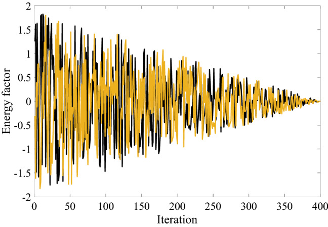
Energy factor (transition factor)

The energy factor controls the changing phases between exploration and exploitation behaviours. The factor is described in Eq. (49). When the factor $E$ is > 1, the exploration stage is performed, and when is < 1, the exploitation phase is carried out.

E = 2 E_{0} (1 - t / T),

where $E_{0}$ is the initial energy which is randomly chosen between ( − 1,1), $T$ is the maximum iteration number, and $t$ is the current iteration. The energy factor is plotted against the iteration number in Fig. 4.

Exploitation (intensification) stage

In this stage, the Harris hawks birds utilize diverse hunting strategies. These exploitation strategies contain 4 main attacking movements: soft besiege, hard besiege, soft besiege with progressive rapid dives, and hard besiege with progressive rapid dives. These four exploitation techniques are defined as follows:

Exploitation’s technique 1(Soft besiege)

In this situation, the prey is confused and looks for a way to escape. This strategy is performed when $r \geq 0.5$ , $|E| \geq 0.5$ , which means that the prey is very exhausted. This tactic is modelled as

\begin{matrix} X (t + 1) & = Δ X (t) - E |J X_{r a n d} (t) - X (t)|, \\ Δ X (t) & = X_{r a n d} (t) - X (t), \\ J & = 2 (1 - r_{5}) . \end{matrix}

where $Δ X (t)$ denotes the location of the tired prey, J is a factor to show the prey’s behaviour, and $r_{5}$ is randomly chosen from [0,1].

Exploitation’s technique 2 (hard besiege)

This tactic happens when $r \geq 0.5$ , $|E| \geq 0.5$ . A killer method as a surprise pounce is executed in this part and can be mathematically presented as Eq. (51):

X (t + 1) = X_{r a b b i t} (t) - E |Δ, X, (t)| .

Exploitation’s technique 3 (Soft besiege with progressive rapid dives)

When $r < 0.5$ , and $|E| \geq 0.5$ , the Harris hawk birds perform their next action based on the following expression:

Y = X_{r a b b i t} (t) - E |J X_{r a b b i t} (t) - X (t)|,

\begin{matrix} Z & = Y + S \times L F (D), \\ L F (x) & = \frac{u \times σ}{{|v|}^{\frac{1}{β}}}, σ = {(\frac{g \times \sin (\frac{π β}{2})}{g \times β \times 2^{(\frac{β - 1}{2})}})}^{\frac{1}{β}}, \end{matrix}

where $LF$ is known as the levy flight function, $S$ is the random vector, $D$ is the number of search agents. $u$ and $v$ are chosen from [0,1] and $β$ is equal to 1.5. To update the positions of search agents, the following expression proposed:

X (t + 1) = \{\begin{matrix} Y i f F (Y) < F (X, (t)) \\ Z i f F (Z) < F (X, (t)) \end{matrix}),

where $Y$ and $Z$ are computed from Eq. (52) and Eq. (53).

Exploitation’s technique 4 (hard besiege with progressive rapid dives)

In the last tactic of the exploitation phase, the Harris Hawks, as search agents for the optimizer, are very close to the prey and kill it. This strategy is explained according to Eq. (55) and Eq. (56):

X (t + 1) = \{\begin{matrix} Y i f F (Y) < F (X, (t)) \\ Z i f F (Z) < F (X, (t)) \end{matrix}),

\begin{matrix} Y & = X_{r a b b i t} (t) - E |J X_{r a b b i t} (t) - X_{m} (t)|, \\ Z & = Y + S \times L F (D) . \end{matrix}

The flowchart of the HHO process is given in Fig. 5.

Proposed enhanced Harris hawks (EHHO)

The mathematical formulation and procedure of the enhanced version of the Harris hawk optimization algorithm are elaborated in this part. Based on the no free lunch (NFL) theory, not every algorithm applies to all problems. For instance, initialization in the HHO algorithm is based on arbitrary numbers, generating a mature population. Furthermore, the proposed strategies used in HHO for updating the population are limited for several applications. Plus, this algorithm is trapped in the local optimum. To enhance the performance of the HHO algorithm and improve the exploitation and exploration phases of the main algorithm, the following methods are added to the HHO algorithm: (1) chaotic method, (2) update besiege strategy 3, (3) update besiege strategy 4, (4) Gaussian mutation, and (5) CLS with a shrinking mode. The first two techniques are presented to assistant the HHO algorithm in generating a different mature population; the third technique is added to the HHO algorithm to enhance its performance for updating the population, and the last two techniques are added to the main HHO algorithm to prevent it from being trapped in the local optimum.

Chaotic method

The initialization in the optimization algorithms is responsible for spreading the design variables in the design space, which can lead to the convergence of the algorithm to the global optimum. The chaotic initialization approach is a powerful procedure that helps the algorithm to generate a more diverse population. The chaotic method has been employed in a wide range of engineering problems, such as feature selection and chaos control [94, 95]. A large number of chaotic maps [96], such as the Chebyshev map, circle map, and intermittency map, are available in the literature. Herein, a prominent logistic map is used, which is described as follows:

β_{i + 1} = μ β_{i} * (1 - β_{i}), i = 1, 2, \dots, S - 1,

where $μ = 4$ is a controlling factor $, β_{1}$ is an arbitrary number between 0 and 1, and $S$ is the number of search agents. To achieve a population with better quality, after the first arbitrary initialization in the main HHO algorithm, chaotic mapping is performed. This modification improves the convergence of the algorithm [97]. This disturbance can then be obtained using the following formulation:

X_{i}^{c} = β_{i} X_{i},

where $X_{i}^{c}$ is the position of the ith Harris hawk with chaotic disturbance, and $β_{i}$ is the ith value in the chaotic sequence.

Update besiege strategy 3

To effectively update the location in Strategy 3 of the standard HHO algorithm, instead of utilizing a soft besiege with rapid progressive dives, a formulation from the flower pollination optimization algorithm is utilized [20]. This approach can be developed as follows [98]:

\begin{matrix} Y & = X (t) + L F (X_{r a b b i t} (t) - X (t)), \\ Z & = X (t) + ε (X_{j} (t) - X_{k} (t)), \\ X (t + 1) & = \{\begin{matrix} Y i f F (Y) < F (X, (t)) \\ Z i f F (Z) < F (X, (t)) \end{matrix}), \end{matrix}

where $ε$ denotes an arbitrary number between 0 and 1, and $X_{j} (t)$ and $X_{k} (t)$ represent pollens from the jth and kth flowers of the identical population, respectively. This technique can enhance the performance of the HHO algorithm to present a more diverse solution in the next iteration.

Update besiege strategy 4

In this section, to improve the performance of the HHO algorithm, a mutation vector extracted from the 2-Opt algorithm and differential evolution algorithm (DE) [99, 100] is replaced by hard besiege with a rapid progressive diving technique. This approach can be expressed as follows:

\begin{matrix} X (t + 1) & = \{\begin{matrix} X_{α} (t) + F (X_{β} (t) - X_{γ} (t)) f (X_{α}, (t)) < f (X_{β}, (t)) \\ X_{β} (t) + F (X_{α} (t) - X_{γ} (t)) o t h e r w i s e \end{matrix},) \\ F & = 1.2 \times β^{t} - 1, \end{matrix}

where $F$ is a parameter that strikes an equilibrium between the local and the global capacity of the enhanced version of the HHO algorithm. $X_{α} (t)$ , $X_{β} (t)$ , and $X_{γ} (t)$ are selected from the population. $β^{t}$ is an arbitrary number between 0 and 1. This method aims to restrict the rising exploitation and prevents being trapped in local optima [60].

Gaussian mutation

Another approach employed in this study to enhance the diversity of the solution is the Gaussian mutation. This strategy has been adopted in a wide range of metaheuristic algorithms to create diversity in solutions [97, 101]. The main purpose of the Gaussian mutation is to boost the global search. Gaussian mutation makes a slight arbitrary change in the group of search agents to prevent trapping in the local optima, leading to more exploitation ability and better convergence. Considering the average of 0 and the standard deviation of 1, a random variable is formed. The Gaussian density function can be formulated as follows [97]:

f_{g a u s s i a n (0, σ^{2})} (α) = \frac{1}{\sqrt{2 π σ^{2}}} e^{- \frac{α^{2}}{2 σ^{2}}},

where $σ^{2}$ indicates the variance, and $α$ represents an arbitrary Gaussian value between [0,1]. The standard deviation is considered to be equal to 1. The Gaussian function with various standard deviation rates is demonstrated in Fig. 6. In the proposed algorithm, firstly, the population is updated according to the energy escaping factor and besiege methods; then, a new population of Harris hawks is created based on Eq. (62):

X^{'} (t) = X (t) * (1 + G (α)),

where $X^{'} (t)$ denotes the location of the new population in each iteration. $G (α)$ represents the Gaussian step vector according to the Gaussian density presented in Eq. (61).

Fig. 6 — Gaussian function for different values of standard deviation

CLS with shrinking mode

Local search (LS) is one of the most efficient strategies for preventing algorithms from being trapped in local optima. It is essential to scour the final solution’s vicinity since, most of the time, the solution is in the neighbourhood of local optima, and the algorithm cannot detect it. Consequently, adding LS to the main HHO algorithm can significantly enhance the performance of the algorithm. Note that, sometimes, LS is not sufficient and would not lead to desirable results. Thus, a chaotic local search (CLS) can be utilized. Since there is randomicity in chaos, CLS can lead to immature convergence [97]. The CLS strategy is added in the last step of the algorithm to detect the best solution. The CLS approach can be formulated as follows:

\begin{matrix} X_{k}^{' (c)} & = (1 - λ) X^{*} + λ (L B + β_{k} (U B - L B)), \\ λ & = 1 - {|\frac{t - 1}{t}|}^{m}, \end{matrix}

where $X_{k}^{' (c)}$ is the kth new location created by CLS, $X^{*}$ shows the best rabbit found so far, $β_{k}$ is the signal generated in the kth chaos, and LB and UB represent the lower and upper limits of the search space, respectively. $λ$ denotes the shrinking scale factor, and t is the current iteration. $m$ is used to handle the shrinking rate and is equal to 1500. Figure 7 depicts the flowchart of the enhanced version of the Harris hawk algorithm (EHHO).

Fig. 7 — The flowchart of the EHHO algorithm

Results and discussions

In this section of the study, first, the simulated experiment’s outcome is presented, and the manner every element of the proposed algorithm can affect the promotion of the final result is examined in detail. Also, the results are compared with the value from the existing catalog. For checking the proposed algorithm's capability, some of the famous engineering problems are chosen to be examined under the proposed algorithm.

Optimum design of TRB

For performing the optimization process, every variable’s limit should be identified in the first calculation stage not to exceed the reasonable number. Maximum and minimum values of each variable used in the design of TRB are computed based on Constraints 1–8 (Table 5). The reported limitation of variables in Table 5 is used as the boundaries of the design variables in optimization algorithms, which include enhanced Harris hawk (EHHO), standard Harris hawk (HHO), whale algorithm (WOA, and sine cosine algorithm (SCA). Different algorithms, including the best solution with their optimum variables, are summarised in Tables 6, 7 for ten different tapered roller bearings. In Tables 6, 7, results are ranked based on the value of dynamic load capacity. It is seen from the results that the introduced enhanced Harris hawk optimization algorithm has superior capability in finding the maximum dynamic load capacity as the optimum outcome and ranks first among the other algorithms. After the enhanced Harris hawk algorithm, the standard Harris hawk has better convergence toward the maximum solution among the rest of the algorithms. It is noteworthy that all values of dynamic load capacity are significantly improved, among which bearing number 30205 has higher improvement (29.4%), and bearing number 32208 has the lowest improvement (16.6%).

Table 5.

Lower and upper limits for optimization design variables

Bearing number	Design variables
	$D_{m}$ (mm)		$D_{r}$ (mm)		$l_{e}$		$Z$		$K_{D_{\min}}$		$K_{D_{\max}}$		$ε$		$e$		$β$
	L.L	U.L	L.L	U.L	L.L	U.L	L.L	U.L	L.L	U.L	L.L	U.L	L.L	U.L	L.L	U.L	L.L	UL
30204	22	45	1.5452	11.8003	1.5452	10.7741	5	91	0.3	0.4	0.5	0.6	0.4	0.5	0.01	0.07	0.80	0.95
30205	27	50	1.6390	11.5	1.6390	11.8539	7	95	0.3	0.4	0.5	0.6	0.4	0.5	0.01	0.07	0.80	0.95
32205	27	50	1.8028	11.5	1.8028	14.4848	7	87	0.3	0.4	0.5	0.6	0.4	0.5	0.01	0.07	0.80	0.95
322/28	30	56	1.9435	13	1.9435	15.4870	7	90	0.3	0.4	0.5	0.6	0.4	0.5	0.01	0.07	0.80	0.95
32206	32	60	2.0903	14	2.0903	15.9770	7	90	0.3	0.4	0.5	0.6	0.4	0.5	0.01	0.07	0.80	0.95
30207	38	69	2.1132	15.5	2.1132	13.4001	7	102	0.3	0.4	0.5	0.6	0.4	0.5	0.01	0.07	0.80	0.95
30306	33	69	2.2023	18	2.2023	14.4075	5	98	0.3	0.4	0.5	0.6	0.4	0.5	0.01	0.07	0.80	0.95
32207	38	69	2.3992	15.5	2.3992	17.5231	7	90	0.3	0.4	0.5	0.6	0.4	0.5	0.01	0.07	0.80	0.95
30307	39	77	2.4967	19	2.4967	16.0424	6	96	0.3	0.4	0.5	0.6	0.4	0.5	0.01	0.07	0.80	0.95
32208	43	77	2.5541	17	2.5541	17.5231	7	94	0.3	0.4	0.5	0.6	0.4	0.5	0.01	0.07	0.80	0.95

Open in a new tab

Table 6.

Optimization parameters for TRB design

Bearing number	Rank	Optimization method	Optimum parameters									Cost
Bearing number	Rank	Optimization method	$D_{m}$ (mm)	$D_{r}$ (mm)	$l_{e}$	$Z$	$K_{D_{m i n}}$	$K_{D_{\max}}$	$ε$	$e$	$β$	$C_{d}$ (N)
30204	1	EHHO	33.0749	7.2313	10.7305	14	0.3940	0.5933	0.4656	0.07	0.95	34,538.3
	2	HHO	33.9860	6.3966	10.3566	16	0.4	0.6	0.5	0.07	0.9403	32,557.6
	3	WOA	34.3789	5.9630	10.5196	17	0.4	0.6	0.5	0.0521	0.95	31,982.2
	4	SCA	33.6178	6.6400	10.0329	15	0.4	0.5352	0.4814	0.07	0.95	31,500.8
	5	GA [2]	34.999	5.29	10.0	20	0.3306	0.5847	0.4507	0.0623	0.9465	31,220
30205	1	EHHO	38.1566	6.4914	11.8460	18	0.4	0.5980	0.4507	0.0699	0.9440	39,864.3
	4	HHO	39.4099	5.4227	11.0261	22	0.3126	0.5792	0.4827	0.0679	0.9059	36,069.5
	2	WOA	38.3892	6.2773	11.7593	18	0.3649	0.5978	0.4982	0.07	0.9466	38,224.3
	3	SCA	38.1955	6.6053	10.8431	17	0.3	0.6	0.4	0.0103	0.8549	36,322.9
	5	GA [2]	39.366	5.38	11.0	21	0.3011	0.5479	0.4658	0.0575	0.9447	34,810
32205	1	EHHO	37.8752	6.0067	14.4667	20	0.4	0.6	0.5	0.0660	0.95	44,818.5
	2	HHO	38.6718	5.2887	14.1878	23	0.3759	0.5602	0.4522	0.0103	0.8888	42,703.4
	4	WOA	38.5210	5.7723	13.2257	22	0.3847	0.6	0.5	0.07	0.95	41,498.6
	3	SCA	38.0050	5.8745	13.9157	20	0.3268	0.5129	0.4054	0.0104	0.95	42,449.7
	5	GA [2]	38.646	5.38	13.0	22	0.3278	0.5978	0.4464	0.0517	0.9494	40,600
322/28	1	EHHO	42.2922	6.6763	15.3855	20	0.3999	0.5920	0.5	0.0106	0.9470	52,898.5
	3	HHO	42.6596	6.3735	15.0591	22	0.3314	0.5824	0.4865	0.0679	0.9145	51,313.4
	2	WOA	42.6949	6.3743	15.0751	21	0.3697	0.5724	0.4731	0.0697	0.9310	51,360.6
	4	SCA	42.6438	6.5608	14.6048	20	0.3258	0.5	0.4	0.0604	0.95	49,833.0
	5	GA [2]	42.839	6.14	14.0	21	0.3260	0.5987	0.4683	0.0699	0.9499	485,400
32206	1	EHHO	45.4239	8.1034	15.9621	17	0.3999	0.5998	0.4976	0.0699	0.9493	61,182.7
	3	HHO	46.1074	7.8389	14.2253	18	0.4	0.6	0.4157	0.0245	0.95	56,315.1
	4	WOA	45.9059	7.8566	14.9822	17	0.4	0.6	0.5	0.0390	0.95	56,317.9
	2	SCA	46.0303	7.7433	14.8871	18	0.3946	0.6	0.4523	0.0109	0.95	57,582.7
	5	GA [2]	47.329	6.37	15.0	21	0.3647	0.5993	0.4983	0.0666	0.9495	52,250

Open in a new tab

Bold values indicate the best results

Table 7.

Optimization results for TRB design

Bearing number	Rank	Optimization method	Optimum parameters									Cost
Bearing number	Rank	Optimization method	$D_{m}$ (mm)	$D_{r}$ (mm)	$l_{e}$	$Z$	$K_{D_{m i n}}$	$K_{D_{\max}}$	$ε$	$e$	$β$	$C_{d}$ (N)
30207	1	EHHO	53.8069	9.1539	13.0691	18	0.356722	0.5213	0.4974	0.0514	0.9142	62,084.4
	2	HHO	53.3063	9.6201	12.5616	17	0.361756	0.5476	0.4572	0.0101	0.8666	60,868.1
	4	WOA	56.1596	6.9678	11.9946	24	0.300363	0.5006	0.4860	0.0339	0.8010	53,606.8
	3	SCA	53.3906	9.5264	12.2235	17	0.36438	0.5359	0.4689	0.0188	0.8322	58,961.8
	5	GA [2]	56.117	6.89	13.0	23	0.3305	0.5027	0.4666	0.0699	0.9417	54,510
30306	1	EHHO	51.5299	10.4971	14.3968	15	0.371458	0.5983	0.4822	0.0393	0.9432	68,439.6
	2	HHO	52.2482	9.8508	14.0246	16	0.325396	0.6	0.5	0.0697	0.9076	65,748
	4	WOA	52.1721	10.0208	13.2669	15	0.378517	0.6	0.5	0.0256	0.95	61,105.3
	3	SCA	51.8496	10.3815	13.2908	15	0.330331	0.5463	0.4084	0.0605	0.9085	63,557.4
	5	GA [2]	54.221	7.74	14.0	20	0.3451	0.5597	0.4999	0.0699	0.9498	59,350
32207	1	EHHO	53.2245	9.0549	17.5122	18	0.397334	0.5969	0.4998	0.0556	0.9463	77,162.2
	4	HHO	55.4309	6.9632	16.9182	24	0.300001	0.5000	0.4630	0.0687	0.8663	70,135.9
	2	WOA	53.0241	9.5731	16.2293	17	0.315465	0.5536	0.4555	0.0548	0.8974	73,982.6
	3	SCA	53.2925	9.1628	16.7300	17	0.311826	0.5757	0.4844	0.0666	0.95	72,252
	5	GA [2]	54.381	7.99	16.0	20	0.3516	0.5968	0.4678	0.678	0.9204	69,810
30307	1	EHHO	58.0431	11.8241	16.0144	15	0.309913	0.5864	0.4378	0.07	0.95	84,483.3
	5	HHO	60.1575	10.1419	13.8516	18	0.367968	0.5022	0.4115	0.0574	0.9387	73,329.2
	3	WOA	60.4662	9.6153	14.6739	20	0.371041	0.5549	0.4623	0.0438	0.8433	75,411.3
	2	SCA	56.9436	12.8484	15.2605	13	0.3776	0.6	0.4	0.0688	0.95	79,927.4
	4	GA [2]	60.875	8.77	15.0	20	0.3545	0.5823	0.4853	0.0643	0.9043	74,940
32208	1	EHHO	59.7637	10.1674	17.5122	18	0.399854	0.5965	0.4987	0.0303	0.95	87,259.1
	4	HHO	60.2563	9.6762	15.6860	20	0.30076	0.5012	0.4891	0.0693	0.8020	79,052.7
	2	WOA	60.4622	9.7165	16.4699	19	0.4	0.6	0.5	0.0607	0.9498	82,458.4
	3	SCA	59.5876	10.4600	16.1836	17	0.308451	0.6	0.4	0.0479	0.9116	81,068.9
	5	GA [2]	60.800	9.06	15.0	20	0.3847	0.5988	0.4517	0.0390	0.8626	75,420

Open in a new tab

Bold values indicate the best results

Moreover, in the results obtained by the enhanced Harris hawk optimization algorithm, it can be seen that although some bearing cases have lower roller numbers, they show better efficiency in terms of fatigue life. Therefore, having a higher number of rollers does not guarantee better fatigue life. Some parameters related to internal geometry which are obtained during the optimization process are summarized in Tables 8, 9.

Table 8.

Optimum internal geometry obtained by different optimization algorithms

Bearing number	Optimization method	Optimum parameters of internal geometry
Bearing number	Optimization method	$S_{2_{m i n}}^{o}$ (mm)	$S_{1_{m i n}}^{i}$ (mm)	$B_{1_{m i n}}$ (mm)	$B_{2_{m i n}}$ (mm)	$C_{1_{m i n}}$ (mm)	$C_{2_{m i n}}$ (mm)	$α_{f}$ degree	$β^{o}$ degree
30204	EHHO	2.2030	2.2030	1.0400	2.3337	1.0339	0.5	8.7777	2.3134
	HHO	2.2030	3.0515	1.2920	2.4685	1.4004	0.5	9.2694	2.0416
	WOA	2.2030	3.4253	1.0686	2.5396	1.2424	0.5	9.5160	1.9047
	SCA	2.3026	2.7863	1.2104	2.8651	1.2823	0.9332	9.1177	2.1261
	GA [2]	2.437	3.665	1.509	3.603	1.703	1.520	9.757	1.693
30205	EHHO	2.3075	2.3745	1.0144	2.3113	1.0004	0.5	10.3736	2.0283
	HHO	2.3075	3.5346	1.6393	2.5202	1.7984	0.5	10.9930	1.6864
	WOA	2.3075	2.5903	1.0648	2.3517	1.0850	0.5	10.4966	1.9603
	SCA	2.3536	2.4301	1.8304	2.4816	1.7893	0.6843	10.3245	2.0569
	GA [2]	2.352	3.534	1.475	2.710	1.642	0.681	10.79	1.676
32205	EHHO	1.5837	1.6465	1.4182	2.6248	1.0000	0.5	16.0377	2.8668
	HHO	1.5837	2.3463	1.5138	2.8495	1.2640	0.5	16.6748	2.5172
	WOA	1.6002	2.2189	2.5027	2.7563	2.1172	0.5423	16.2961	2.7283
	SCA	1.6829	1.8344	1.6553	2.9283	1.2598	0.7550	16.1557	2.8034
	GA [2]	1.766	2.463	2.192	3.307	1.901	0.969	16.71	2.558
322/28	EHHO	1.9662	1.9662	1.6443	2.4794	1.0782	0.5	15.5429	2.7660
	HHO	1.9870	2.3064	1.8310	2.6277	1.3302	0.5554	15.7802	2.6362
	WOA	1.9662	2.3211	1.8718	2.5717	1.3707	0.5	15.7831	2.6346
	SCA	1.9841	2.2846	2.3161	2.5713	1.7631	0.5476	15.6578	2.7048
	GA [2]	2.197	2.627	2.222	3.272	1.763	1.116	16.00	2.541
32206	EHHO	2.3840	2.3840	1.3077	2.952969	1.0039	0.5	10.2180	2.1123
	HHO	2.3840	2.9840	2.9680	3.013218	2.6907	0.5	10.3759	2.0271
	WOA	2.3840	2.8116	2.2291	3.004961	1.9558	0.5	10.3532	2.0387
	SCA	2.3893	2.9304	2.2828	3.047944	2.0271	0.5212	10.4075	2.0088
	GA [2]	2.401	4.154	1.897	3.358	1.873	0.568	10.80	1.654

Open in a new tab

Table 9.

Optimum internal geometry obtained by different optimization algorithms

Bearing number	Optimization method	Optimum parameters of internal geometry
Bearing number	Optimization method	$S_{2_{m i n}}^{o}$ (mm)	$S_{1_{m i n}}^{i}$ (mm)	$B_{1_{m i n}}$ (mm)	$B_{2_{m i n}}$ (mm)	$C_{1_{m i n}}$ (mm)	$C_{2_{m i n}}$ (mm)	$α_{f}$ degree	$β^{o}$ degree
30207	EHHO	3.0310	3.7907	2.0602	2.0602	1.5009	0.8121	10.3803	2.0283
	HHO	3.1125	3.3767	2.3059	2.3059	1.6669	1.1380	10.1922	2.1331
	WOA	3.0625	6.0366	2.6099	2.6099	2.4212	0.9380	11.2649	1.5385
	SCA	3.1576	3.4895	2.4410	2.5059	1.8146	1.3186	10.2299	2.1126
	GA [2]	3.000	5.955	1.863	2.370	1.695	0.688	10.90	1.524
30306	EHHO	3.5805	4.6056	1.4645	3.2652	1.5018	0.4	8.2577	1.9991
	HHO	3.5805	5.2806	1.7469	3.3612	1.8673	0.4	8.4846	1.8735
	WOA	3.6121	5.2185	2.3656	3.4910	2.4582	0.5508	8.4326	1.9031
	SCA	3.5919	4.8920	2.4862	3.3418	2.5307	0.4543	8.3110	1.9706
	GA [2]	3.643	7.219	1.175	3.988	1.595	0.698	8.797	1.474
32207	EHHO	2.8315	3.1627	2.0059	3.7359	1.5000	0.5	10.3718	2.0283
	HHO	2.8315	5.2111	2.2368	4.1453	2.0808	0.5	11.2268	1.5556
	WOA	2.8315	2.9474	3.3453	3.6495	2.7443	0.5	10.1836	2.1339
	SCA	2.8392	3.2167	2.7584	3.7521	2.2280	0.5309	10.3400	2.0467
	GA [2]	2.962	4.331	2.787	4.471	2.447	1.023	10.69	1.786
30307	EHHO	3.5035	4.5974	1.6982	3.4281	1.5178	0.8	8.2579	1.9992
	HHO	3.5035	6.5665	3.6045	3.6882	3.6380	0.8	8.7935	1.7035
	WOA	3.5254	6.9000	2.6154	3.8705	2.7292	0.9043	8.9430	1.6198
	SCA	3.6216	3.6367	2.0072	3.8521	1.6918	1.3625	7.9418	2.1752
	GA [2]	3.556	7.325	2.069	4.101	2.264	1.050	8.739	1.531
32208	EHHO	3.0175	3.3879	1.7375	4.0043	1.5	0.5	10.3753	2.0283
	HHO	3.2353	4.0084	2.5722	4.9797	2.4025	1.3710	10.5557	1.9299
	WOA	3.0175	4.0227	2.6850	4.0948	2.5127	0.5	10.5523	1.9312
	SCA	3.1223	3.2859	2.6658	4.3794	2.3700	0.9190	10.2781	2.0834
	GA [2]	3.348	4.611	2.685	5.554	2.615	1.825	10.70	1.809

Open in a new tab

The convergence curve of the optimization algorithms shows how to obtain the final result (Fig. 8). Better performance of EHHO than other algorithms is seen obviously. One of the main reasons for this high-quality result is to have a mature population at the beginning of the optimization process, which is attributed to the chaotic initialization. Another reason for the improved efficiency is due to using the flower pollination and 2-Opt algorithms. Using two other techniques, Gaussian mutation and chaotic local search, can facilitate the optimization process for finding the optimum solution at the end of the algorithm. Local optimum is a significant obstacle experienced by most algorithms; having an efficient structure for avoiding local optima is one of the advantages of suitable algorithms. Using a chaotic local search technique can assist the algorithm in preventing falls in the local optima. It is noteworthy that the structure of SCA is not appropriate for this TRB problem and has minimum convergence result compared to the other algorithms.

To see the proficiency of the algorithms in more detail, a statistical analysis is performed for some cases of tapered roller bearings. Table 10 shows the result of this analysis in terms of standard deviation (STD), worst solution, and best mean. The result of statistical analysis demonstrates that the EHHO has the lowest STD among the other algorithms. The lowest STD demonstrates that EHHO can easily find the maximum solution in every run of the optimization process and proves the robustness of this algorithm. Also, the best, mean, and worst solutions belong to the EHHO algorithm. After the EHHO algorithm, the SCA ranks second in terms of the lowest STD; however, SCA obtains the lowest best result.

Table 10.

Statistical results for four optimization algorithms

Bearing number	Optimization method	Best	Mean	Worst	STD
30204	EHHO	34,538.27	34,113.06	32,818.62	530.10
	HHO	32,557.60	25,667.99	17,659.57	5590.53
	WOA	31,982.23	27,132.90	20,411.60	3410.19
	SCA	31,500.79	30,394.68	28,808.47	852.50
30205	EHHO	39,864.26	39,616.49	38,925.36	326.06
	HHO	36,069.50	24,354.68	17,916.79	6067.16
	WOA	38,224.26	32,832.10	27,058.17	3565.19
	SCA	36,641.31	35,693.81	34,614.29	746.37
32205	EHHO	44,818.52	44,619.33	43,782.81	413.32
	HHO	42,703.37	34,546.78	19,051.47	8463.81
	WOA	41,498.62	36,313.34	20,771.22	7514.12
	SCA	42,449.72	40,926.80	39,385.14	1092.16
322/28	EHHO	52,898.87	52,747.44	51,864.48	338.20
	HHO	51,313.38	38,916.64	26,217.00	9552.93
	WOA	51,360.63	40,454.10	27,595.49	8753.15
	SCA	49,833.04	47,829.98	46,190.28	1294.12

Open in a new tab

Bold values indicate the best results

LL lower limit, UL upper limit

Figure 9 compares the design variables from the enhanced Harris hawk algorithm (EHHO), genetic algorithm (GA), and the standard catalogue. The graph in Fig. 9 shows that the EHHO algorithm successfully maximizes the fatigue life of bearing with a lower number of rollers. Also, Fig. 9 shows that the EHHO algorithm uses a higher mean diameter value and has sufficient length compared to GA and bearing standard.

Fig. 9 — Comparison of design variables: standard catalog, GA, and EHHO

Stability evaluation is one of the vital steps of performance verification [102, 103]. For quality evaluation metrics [104], we considered the average of solutions as the primary metric to judge the accuracy of the performance. We fixed fair judgments as per references [24, 85, 105, 106]. For having an exhaustive vision of the proposed algorithm, different algorithms are created with separate techniques used in EHHO. These algorithms are created based on techniques including chaotic initialization, Gaussian mutation, deferential evaluation, pollination algorithm, and chaotic local search mentioned in the optimization methodology section. The optimization process is performed for these algorithms in 500 iterations, and the results are summarized in Table 11. The convergence curves are shown in Fig. 10, in which using strategies of chaotic local search, chaotic initialization, and Gaussian mutation with standard HHO does not affect the accuracy significantly. By replacing the pollination algorithm and deferential evolution formulation with the hunting strategies of the Harris hawk algorithm, the results improve significantly. The EHHO, which is a combination of all the mentioned techniques, has the best results compared to the other ten algorithms in terms of precision, and its performance is not trapped to local optima. The STD result of EHHO also illustrates the performance of every element of this algorithm.

Table 11.

Statistical result for tapered roller bearing

Bearing number	Optimization method	Best	Mean	Worst	STD
32207	HHO	68,199.43	50,422.74	42,447.67	8681.153
	Cha-HHO	66,916.79	48,827.31	44,035.26	7836.42
	Gau-HHO	62,472.2	55,858.61	52,381.36	3833.961
	CLS-HHO	58,549.38	51,582.96	34,497.03	9443.249
	Cha-Gau-CLS-HHO	63,363.86	54,171.72	45,688.48	5623.82
	DE-Pol-HHO	72,777.02	69,517.8	65,042.16	2953.21
	Cha-DE-Pol-HHO	74,132.74	69,715.49	65,524.29	2753.776
	Gau-DE-Pol-HHO	76,651.93	73,863.27	65,384.35	3386.548
	CLS-DE-Pol-HHO	73,378.96	68,353.78	62,805.36	3852.129
	EHHO	77,091.46	75,709.29	73,063.19	1264.924
30307	HHO	62,170.57	45,428.87	39,287.2	8619.527
	Cha-HHO	74,761.57	53,460.88	49,441.91	8823.459
	Gau-HHO	65,172.04	57,959.72	50,047.24	3569.721
	CLS-HHO	66,477.57	57,054.35	56,007.32	3310.984
	Cha-Gau-CLS-HHO	77,002.43	59,512.23	53,099.14	9651.839
	DE-Pol-HHO	79,627.92	71,732.16	46,078.51	10,340.03
	Cha-DE-Pol-HHO	81,008.2	76,080.66	68,414.83	4466.655
	Gau-DE-Pol-HHO	81,417.25	76,767.38	59,460.96	6366.401
	CLS-DE-Pol-HHO	81,663.6	74,097.82	70,330.55	3768.046
	EHHO	83,036.86	78,970.02	75,167.9	2782.379
32208	HHO	73,873.29	56,993.26	42,935.66	8777.11
	Cha-HHO	74,331.65	57,761.36	54,570.15	6962.738
	Gau-HHO	70,593.91	60,848.55	55,732.52	6369.845
	CLS-HHO	68,139.23	59,715.36	46,030.73	7312.302
	Cha-Gau-CLS-HHO	71,781.09	67,488.67	65,621.82	1777.807
	DE-Pol-HHO	83,381.08	77,385.17	70,067.29	4811.884
	Cha-DE-Pol-HHO	85,393.4	78,315.92	68,618.12	6102.392
	Gau-DE-Pol-HHO	85,506.08	83,351.81	78,067.71	2574.536
	CLS-DE-Pol-HHO	84,901.93	76,804.31	66,011.37	5429.324
	EHHO	86,603.7	84,233.2	80,135.14	2476.326

Open in a new tab

Bold values indicate the best results

Fig. 10 — Convergence curve for ten algorithms. a 32207, b 30307 c 32208

Engineering problems

There are many problems that their feature space is more complex than the assessed benchmark spaces [107–111]. Despite benchmark cases, engineering problems always involve some variables that are constrained [28, 112–115]. For testing and benchmarking the proposed algorithm, some popular and perplexing engineering functions are common in the literature. These engineering functions can challenge every optimization algorithm with their complexity in their structure. Most of these problems have more than three variables and constraints with many local optima. In this part of the paper, five well-known and challenging engineering problems are evaluated by the EHHO algorithm to examine the effectiveness and capability of this algorithm. The aspects of the engineering problems are described in the next subsections.

Cantilever beam

Figure 11 shows the structure of this benchmarked problem. This beam is exposed to the load at the right end. Five variables of beam design contain the vertical length of the connected boxes. The range of the variables is from 0 to 100. The target is to minimize the weight of the entire design. The optimization scheme of this problem is given in Eq. (64) below:

\begin{matrix} \vec{x} = [h_{1}, h_{2}, h_{3}, h_{4}, h_{5}], \\ M i n i m i z e : f (\vec{x}) = 0.0624 (x_{1} + x_{2} + x_{3} + x_{4} + x_{5}), \\ S u b j e c t t o : G (\vec{x}) = \frac{61}{x_{1}^{3}} + \frac{37}{x_{2}^{3}} + \frac{19}{x_{3}^{3}} + \frac{7}{x_{4}^{3}} + \frac{1}{x_{5}^{3}} - 1 \leq 0, \\ 0 \leq x_{i} \leq 100 . \end{matrix}

The optimum solution of beam design is reported in Table 12. Moreover, Table 12 contains the optimum design results of other algorithms such as the modified firefly algorithm [116], crow search (CS) [117], and symbiotic organisms search (SOS) [118], and the standard Harris Hawk on the beam structure. The EHHO found 1.33995825 as the optimal solution of weight for the cantilever beam design, indicating the efficiency of this algorithm compared to the modified firefly algorithm, crow search algorithm, and symbiotic organisms algorithm. This case may be handy for building structures and how engineers can deal with a component [119].

Table 12.

Comparison results for cantilever beam design

Optimization method	Optimum variables					Optimum cost
Optimization method	$h_{1}$	$h_{2}$	$h_{3}$	$h_{4}$	$h_{5}$	Weight
EHHO	6.0143	5.3029	4.4964	3.5053	2.1548	1.33995825
HHO	6.1016	5.343	4.4237	3.4533	2.1582	1.3403595
MFA [116]	5.98487	5.3167269	4.49733	3.5136165	2.161620	1.3399881
CS [117]	6.0089	5.3049	4.5023	3.5077	2.1504	1.33999
SOS [118]	6.01878	5.30344	4.49587	3.49896	2.15564	1.33996

Open in a new tab

Bold value indicates the best results

Pressure vessel

The cost of construction of every piece of equipment is substantial for manufacturers, and the minimization of expenses can be formulated as an interesting problem. The variables' vector of the pressure vessel problem contains some critical parameters such as the thickness of the head and shell ( $T_{s}$ and $T_{h}$ , respectively) and cylindrical curvature radius ( $r$ ) and distance ( $L$ ). The limitation of the first and second variables is between 0 and 99, and the criteria for the third and fourth variables are between 10 and 200. The layout for this structure is as follows:

\begin{matrix} \vec{x} = [x_{1}, x_{2}, x_{3}, x_{4}] = [T_{s}, T_{h}, R, L], \\ M i n i m i z e : f (\vec{x}) = 0.6224 x_{1} x_{3} x_{4} + 1.7781 x_{1}^{2} x_{4} + 3.1661 x_{4} x_{1}^{2} + 19.84 x_{4} x_{1}^{2}, \\ S u b j e c t t o : h_{1} (\vec{x}) = - x_{1} + 0.0193 x_{3} \leq 0, \\ h_{2} (\vec{x}) = - x_{2} + 0.00954 x_{3} \leq 0, \\ h_{3} (\vec{x}) = - π x_{4} x_{3}^{2} - \frac{4}{3} π x_{3}^{3} + 1296000 \leq 0, \\ h_{4} (\vec{x}) = x_{4} - 240 \leq 0, \\ 0 \leq x_{1} \leq 99, 0 \leq x_{2} \leq 99, 10 \leq x_{3} \leq 200, 10 \leq x_{4} \leq 200 . \end{matrix}

The result for this problem is presented in Table 13. It is obvious that the fabrication cost of the pressure vessel design related to EHHO is better than that of other algorithms mentioned in Table 13. Note that EHHO has improved the optimal solution by 2% compared to the standard HHO.

Table 13.

Comparison results for pressure vessel design

Optimization method	Optimum variables				Optimum cost
Optimization method	$T_{s}$	$T_{h}$	$r$	$L$	Fabrication cost
EHHO	0.77817	0.38465	40.3196	200	5885.36355
HHO [50]	0.81758	0.40729	42.09174	176.75873	6000.46259
CMVHHO [120]	0.849756	0.421472	43.900722	155.517156	6039.6918
ADHHO [121]	0.87015	0.43114	45.01254	143.5317	6072.56
CCMWOA [97]	0.77966	0.38561	40.34738	199.6141	5895.2039
WOA [88]	0.81250	0.43750	42.09820	176.6389	6059.7410
VPLSCA [122]	0.8152	0.4265	42.0851	176.73154	6042.711935
UBSCIW [123]	0.7798	0.3866	40.3884	199.0685	5889.2305
ESSA [124]	0.781463	0.386278	40.4903	197.63744	5890.9885

Open in a new tab

Bold value indicates the best results

Spring geometry

The objective function of this design problem is to minimize the weight of a tension/compression spring. Shear stress and deflection influence the design of the spring, which can be related to constraints of spring. Three variables of coil number ( $N$ ), cord diameter ( $d$ ), and mean diameter ( $D$ ) are chosen in the design vector to provide the lowest weight for the spring. The range for ( $d$ ) is 0.05–2, for ( $D$ ) is 0.25–1.3, and for the last variable ( $N$ ) is 2–15. The spring formulation is derived as below:

\begin{matrix} \vec{x} = [x_{1}, x_{2}, x_{3}] = [d, D, N], \\ M i n i m i z e : f (\vec{x}) = x_{1}^{2} x_{2} x_{3} + 2 x_{1}^{2} x_{2}, \\ S u b j e c t t o : h_{1} (\vec{x}) = 1 - \frac{x_{2}^{3} x_{3}}{71785 x_{1}^{4}} \leq 0, \\ h_{2} (\vec{x}) = \frac{x_{2}^{3} x_{3}}{12566 (x_{2} x_{1}^{3} - x_{1}^{4})} + \frac{1}{5108 x_{1}^{2}} - 1 \leq 0, \\ h_{3} (\vec{x}) = 1 - \frac{140.45 x_{1}}{x_{2}^{2} x_{3}} \leq 0, \\ h_{4} (\vec{x}) = \frac{x_{1} + x_{2}}{1.5} - 1 \leq 0, \\ 0.05 \leq x_{1} \leq 2, 0.25 \leq x_{2} \leq 1.3, 2 \leq x_{3} \leq 15 . \end{matrix}

Table 14 summarizes the value obtained from the optimization process. The EHHO diminishes the weight to an accuracy of 0.01266 kg compared to the other algorithms such as modified whale algorithm (CCMWOA) [97], enhanced salp swarm (ESSA) [124], whale algorithm (WOA) [88], and modified HHO (GCHHO) [59].

Table 14.

Results for tension/compression spring design

Optimization method	Optimum variables			Optimum cost
Optimization method	$d$	$D$	$N$	Weight
EHHO	0.0516751748	0.356383766	11.30857249	0.012665236
HHO	0.05179	0.3593	11.13885	0.012665443
MHHO [125]	0.051654	0.355881	11.33883	0.01266619
CCMWOA [97]	0.051843	0.360444	11.07410	0.0126660
WOA [88]	0.051207	0.345215	12.0043032	0.0126763
ESSA [124]	0.051719	0.357434	11.247123	0.0126653
GCHHO [59]	0.0516479	0.355729	11.3471231	0.012665264

Open in a new tab

Bold value indicates the best results

Welded beam

There are 4 design variables for the welded beam design optimization problem (thickness, $b$ , height, $t$ , length of the bar, $l$ , with weld $h$ ). There are 7 constraints, and most of them relate to load, stresses on the bar, and end deflection on the spring. The structural formulation, range of variables, and some constant parameters are provided by Eq. (67):

\begin{matrix} \vec{x} & = [x_{1}, x_{2}, x_{3}, x_{4}] = [h, l, t, b], \\ M i n i m i z e : f (\vec{x}) = 1.10471 x_{2} x_{1}^{2} + 0.04811 x_{3} x_{4} (14 + x_{2}), \\ S u b j e c t t o : h_{1} (\vec{x}) = τ (\vec{x}) - τ_{m a x} \leq 0, \\ h_{2} (\vec{x}) = σ (\vec{x}) - σ_{m a x} \leq 0, \\ h_{3} (\vec{x}) = δ (\vec{x}) - δ_{m a x} \leq 0, \\ h_{4} (\vec{x}) = x_{1} - x_{4} \leq 0, \\ h_{5} (\vec{x}) = P - P_{c} (\vec{x}) \leq 0, \\ h_{6} (\vec{x}) = 0.125 - x_{1} \leq 0, \\ h_{7} (\vec{x}) = 0.10471 x_{1}^{2} + 0.04811 x_{3} x_{4} (14 + x_{2}) - 5 \leq 0, \\ 0.1 \leq x_{1} \leq 2, 0.1 \leq x_{2} \leq 10, 0.1 \leq x_{3} \leq 10, 0.1 \leq x_{4} \leq 2, \end{matrix}

where

\begin{matrix} τ (\vec{x}) & = \sqrt{{(τ^{'})}^{2} + 2 τ^{'} τ^{''} \frac{x^{2}}{2 R} + {(τ^{''})}^{2}}, τ^{'} = \frac{P}{\sqrt{2} x_{1} x_{2}}, τ^{''} = \frac{MR}{J}, M = P (L + \frac{x_{2}}{2}), \\ R & = \sqrt{\frac{x_{2}^{2}}{4} + {(\frac{x_{1} + x_{3}}{2})}^{2}}, J = 2 \{\sqrt{2}, x_{1}, x_{2}, [\frac{x_{2}^{2}}{12} + {(\frac{x_{1} + x_{3}}{2})}^{2}]\} \\ σ (\vec{x}) = \frac{6 P L}{x_{4} x_{3}^{2}}, δ (\vec{x}) = \frac{4 P L^{3}}{E x_{3}^{3} x_{4}}, P_{c} (\vec{x}) = \frac{4.013 E \sqrt{\frac{x_{3}^{2} x_{4}^{6}}{36}}}{L^{2}} (1 - \frac{x_{3}}{2 L} \sqrt{\frac{E}{4 G}}) \\ P & = 6000 l b, L = 14 i n, δ_{m a x} = 0.25 i n, E = 30 \times 10^{6} p s i, G = 12 \times 10^{6} p s i, τ_{m a x} 13600 p s i, σ_{m a x} = 30000 p s i . \end{matrix}

The results in Table 15 show the excellence of the proposed algorithm.

Table 15.

Results for welded beam design

Optimization method	Optimum variables				Optimum cost
Optimization method	$h$	$l$	$t$	$b$	Fabrication cost
EHHO	0.2057003	3.4711372	9.03668181	0.20572935	1.72490231
HHO	0.204039	3.531061	9.027463	0.206147	1.73199057
CMVHHO [120]	0.205331	3.4787	9.039544	0.205723	1.726023
WOA [88]	0.205396	3.484293	9.037426	0.206276	1.730499

Open in a new tab

Bold value indicates the best results

Speed reducer

The scheme of the speed reducer is depicted in Fig. 12. The speed reducer shaft is exposed to stress and transverse deflection, and the gear teeth tolerate stresses such as bending stress, which can be considered constraints. The optimization problem for the speed reducer problem has seven variables and 11 nonlinear constraints. The variables are explained in Fig. 12. The formulation for the optimization design of the speed reducer can be expressed in Eq. (68):

\begin{matrix} \vec{x} = [x_{1}, x_{2}, x_{3}, x_{4}, x_{5}, x_{6}, x_{7}], \\ Min : f (\vec{x}) = 0.7854 x_{1} x_{2}^{2} (3.3333 x_{3}^{2} + 14.9334 x_{3} - 43.0934) \\ - 1.508 x_{1} (x_{6}^{2} + x_{7}^{2}) + 7.4777 (x_{6}^{3} + x_{7}^{3}) + 0.7854 (x_{4} x_{6}^{2} + x_{5} x_{7}^{2}), \\ Subject to : h_{1} (\vec{x}) = \frac{27}{x_{1} x_{2}^{2} x_{3}} - 1 \leq 0, \\ h_{2} (\vec{x}) = \frac{397.5}{x_{1} x_{2}^{2} x_{3}^{2}} - 1 \leq 0, h_{3} (\vec{x}) = \frac{1.93 x_{4}^{3}}{x_{2} x_{6}^{4} x_{3}} - 1 \leq 0, \\ h_{6} (\vec{x}) = \frac{1.1 x_{7} + 1.9}{x_{5}} - 1 \leq 0, h_{7} (\vec{x}) = \frac{{[{(\frac{745 x_{5}}{x_{2} x_{3}})}^{2} + 157.5 \times 10^{6}]}^{\frac{1}{2}}}{85 x_{7}^{3}} - 1 \leq 0, \\ h_{8} (\vec{x}) = \frac{x_{2} x_{3}}{40} - 1 \leq 0, h_{9} (\vec{x}) = \frac{5 x_{2}}{x_{1}} - 1 \leq 0 \\ h_{10} (\vec{x}) = \frac{x_{1}}{12 x_{2}} - 1 \leq 0, h_{11} (\vec{x}) = \frac{1.5 x_{6} + 1.9}{x_{4}} - 1 \leq 0, \\ 2.6 \leq x_{1} \leq 3.6, 0.7 \leq x_{2} \leq 0.8, 17 \leq x_{3} \leq 28, 7.3 \leq x_{4} \leq 8.3 \\ 7.3 \leq x_{5} \leq 8.3, 2.9 \leq x_{6} \leq 3.9, 5 \leq x_{7} \leq 5.5 \end{matrix}

The speed reducer’s optimum weight is reported in Table 16 for the algorithms. The EHHO reduces the optimum cost to 2994.4710 kg, which is a competitive result compared to other algorithms.

Table 16.

Results for speed reducer design

Optimization method	Optimum variables							Optimum cost
Optimization method	$x_{1}$	$x_{2}$	$x_{3}$	$x_{4}$	$x_{5}$	$x_{6}$	$x_{7}$	Weight
EHHO	3.5	0.7	17	7.3	7.7153	3.3502	5.2866	2994.4710
HHO	3.50253	0.7	17	7.3	7.9206	3.3538	5.2867	3000.9479
m-HHO [62]	3.5	0.7	17	7.3	7.8	3.35127	5.28668	2996.6162
GLF-GWO [126]	3.5000091	0.7	17	7.3	7.8	3.3502335	5.2866856	2996.3680

Open in a new tab

Bold value indicates the best results

Conclusions and future works

In this paper, a novel algorithm is proposed to enhance the performance of the Harris hawk optimization algorithm (HHO) based on new features, which improve the exploration and exploitation phases of the original HHO algorithm. At first, chaotic initialization is used to explore the search area extensively to cover and generate all possible solutions equally. In this way, a mature population is created. After that, two of the Harris hawk pouncing strategies are changed to generate more appropriate agents for updating the population. Also, the Gaussian strategy makes the update of the population boosted. At the end of the proposed algorithm, a chaotic local search with the shrinking mode is exploited to avoid possible local optima. The proposed algorithm is tested on tapered roller bearings successfully. The objective function is related to the maximization of the fatigue life of TRB. It contains nine variables and 26 constraints. The results show that the best result can be obtained by the application of the enhanced Harris hawk algorithm (EHHO) on the design optimization of the fatigue life of TRB. In addition, the mentioned algorithm is tested on some common engineering problems in the literature. Similarly, the optimization results are improved using the EHHO algorithm compared to the algorithms from the literature. Therefore, the proposed algorithm can be used in complex engineering problems where there are many design variables.

Acknowledgements

This paper results from the MSc thesis of the first name that defended his thesis successfully within the revision of this research. We acknowledge the supports of Ozyegin University. We also acknowledge reviewers’ comments and the editor’s efforts, which significantly enhanced this research’s excellence.

Footnotes

https://aliasgharheidari.com/SMA.html.

https://aliasgharheidari.com/HGS.html.

https://aliasgharheidari.com/RUN.html.

⁴

https://aliasgharheidari.com/HHO.html.

Publisher's Note

Springer Nature remains neutral with regard to jurisdictional claims in published maps and institutional affiliations.

Contributor Information

Ahmad Abbasi, Email: ahmad.abbasi@ozu.edu.tr.

Behnam Firouzi, Email: behnam.firoozi@ozu.edu.tr.

Polat Sendur, Email: polat.sendur@ozyegin.edu.tr.

Ali Asghar Heidari, Email: as_heidari@ut.ac.ir, Email: aliasghar68@gmail.com.

Huiling Chen, Email: chenhuiling.jlu@gmail.com.

Rajiv Tiwari, Email: rtiwari@iitg.ac.in.

References

1.Jat A, Tiwari R. Multi-objective optimization of spherical roller bearings based on fatigue and wear using evolutionary algorithm. J King Saud Univ-Eng Sci. 2020;32(1):58–68. [Google Scholar]
2.Tiwari R, Sunil KK, Reddy R. An optimal design methodology of tapered roller bearings using genetic algorithms. Int J Comput Methods Eng Sci Mech. 2012;13(2):108–127. doi: 10.1080/15502287.2011.654375. [DOI] [Google Scholar]
3.Senthil Kumaran S, Srinivasan K. A review on life increment of tapered roller bearings. J Crit Rev. 2020;7(6):764–775. [Google Scholar]
4.Bhowmick H, Choudhary RTG (2006) Quasi-static analysis of tapered roller bearings and comparison of bearing lives for different roller surface profiles. In: 2nd international congress on computational mechanics and simulation, 2006
5.Hu Y, et al. Corrosion fatigue lifetime assessment of high-speed railway axle EA4T steel with artificial scratch. Eng Fract Mech. 2021;245:107588. doi: 10.1016/j.engfracmech.2021.107588. [DOI] [Google Scholar]
6.Tiwari R, Chandran R (2013) Thermal based optimum design of tapered roller bearing through evolutionary Algorithm. In: Gas turbine India conference, vol 35161. American Society of Mechanical Engineers, p V001T05A021
7.Kumar KS, Tiwari R, Prasad P. An optimum design of crowned cylindrical roller bearings using genetic algorithms. J Mech Des. 2009 doi: 10.1115/1.3116344. [DOI] [Google Scholar]
8.Verma SK, Tiwari R. Robust optimum design of tapered roller bearings based on maximization of fatigue life using evolutionary algorithm. Mech Mach Theory. 2020;152:103894. doi: 10.1016/j.mechmachtheory.2020.103894. [DOI] [Google Scholar]
9.Kalyan M, Tiwari R, Ahmad MS. Multi-objective optimization in geometric design of tapered roller bearings based on fatigue, wear and thermal considerations through genetic algorithms. Sadhana. 2020 doi: 10.1007/s12046-020-01385-3. [DOI] [Google Scholar]
10.Choi D-H, Yoon K-C. A design method of an automotive wheel-bearing unit with discrete design variables using genetic algorithms. J Trib. 2001;123(1):181–187. doi: 10.1115/1.1329878. [DOI] [Google Scholar]
11.Chakraborty I, et al. Rolling element bearing design through genetic algorithms. Eng Optimiz. 2003;35(6):649–659. doi: 10.1080/03052150310001624403. [DOI] [Google Scholar]
12.Dandagwhal R, Kalyankar V. Design optimization of rolling element bearings using advanced optimization technique. Arab J Sci Eng. 2019;44(9):7407–7422. doi: 10.1007/s13369-019-03767-0. [DOI] [Google Scholar]
13.Panda S, et al. Re-examination for effect of ball race conformity on life of rolling element bearing using Metaheuristic. Int J Adv Mech Eng. 2018;8(1):285–294. [Google Scholar]
14.Kang K, et al. Robust design optimization of an angular contact ball bearing under manufacturing tolerance. Struct Multidiscip Optim. 2019;60(4):1645–1665. doi: 10.1007/s00158-019-02335-2. [DOI] [Google Scholar]
15.Tiwari R, Waghole V. Optimization of spherical roller bearing design using artificial bee colony algorithm and grid search method. Int J Comput Methods Eng Sci Mech. 2015;16(4):221–233. doi: 10.1080/15502287.2015.1045998. [DOI] [Google Scholar]
16.Zhou Y, et al. Video coding optimization for virtual reality 360-degree source. IEEE J Select Topics Signal Process. 2019;14(1):118–129. doi: 10.1109/JSTSP.2019.2957952. [DOI] [Google Scholar]
17.Wu C, et al. Differential received signal strength based RFID positioning for construction equipment tracking. Adv Eng Inf. 2019;42:100960. doi: 10.1016/j.aei.2019.100960. [DOI] [Google Scholar]
18.Xue X, et al. Affine transformation-enhanced multifactorial optimization for heterogeneous problems. IEEE Trans Cybernet. 2020 doi: 10.1109/TCYB.2020.3036393. [DOI] [PubMed] [Google Scholar]
19.Ding L, et al. Definition and application of variable resistance coefficient for wheeled mobile robots on deformable terrain. IEEE Trans Rob. 2020;36(3):894–909. doi: 10.1109/TRO.2020.2981822. [DOI] [Google Scholar]
20.Wu C, et al. Critical review of data-driven decision-making in bridge operation and maintenance. Struct Infrastruct Eng. 2020 doi: 10.1080/15732479.2020.1833946. [DOI] [Google Scholar]
21.Jiang Q, et al. Optimizing multistage discriminative dictionaries for blind image quality assessment. IEEE Trans Multimedia. 2017;20(8):2035–2048. doi: 10.1109/TMM.2017.2763321. [DOI] [Google Scholar]
22.Wang B, et al. A kind of improved quantum key distribution scheme. Optik. 2021;235:166628. doi: 10.1016/j.ijleo.2021.166628. [DOI] [Google Scholar]
23.Yang Y, et al. New pore space characterization method of shale matrix formation by considering organic and inorganic pores. J Nat Gas Sci Eng. 2015;27:496–503. doi: 10.1016/j.jngse.2015.08.017. [DOI] [Google Scholar]
24.Bo W, et al. Malicious URLs detection based on a novel optimization algorithm. IEICE Trans Inf Syst. 2021;104(4):513–516. doi: 10.1587/transinf.2020EDL8147. [DOI] [Google Scholar]
25.Alam Z, et al. Experimental and numerical investigation on the complex behaviour of the localised seismic response in a multi-storey plan-asymmetric structure. Struct Infrastruct Eng. 2021;17(1):86–102. doi: 10.1080/15732479.2020.1730914. [DOI] [Google Scholar]
26.Zuo X, et al. The modeling of the electric heating and cooling system of the integrated energy system in the coastal area. J Coast Res. 2020;103(SI):1022–1029. doi: 10.2112/SI103-213.1. [DOI] [Google Scholar]
27.Zhu D, et al. Evaluating the vulnerability of integrated electricity-heat-gas systems based on the high-dimensional random matrix theory. CSEE J Power Energy Syst. 2019;6(4):878–889. [Google Scholar]
28.Zhang Y, et al. Analysis of grinding mechanics and improved predictive force model based on material-removal and plastic-stacking mechanisms. Int J Mach Tools Manuf. 2017;122:81–97. doi: 10.1016/j.ijmachtools.2017.06.002. [DOI] [Google Scholar]
29.Yin F, et al. Multifidelity genetic transfer: an efficient framework for production optimization. SPE J. 2021 doi: 10.2118/205013-PA. [DOI] [Google Scholar]
30.Eshtay M, Faris H, Heidari AA, Ala’M AZ, Aljarah I. AutoRWN: automatic construction and training of random weight networks using competitive swarm of agents. Neural Comput Appl. 2021;33(11):5507–5524. doi: 10.1007/s00521-020-05329-0. [DOI] [Google Scholar]
31.Faris H, et al. An intelligent system for spam detection and identification of the most relevant features based on evolutionary Random Weight Networks. Inf Fus. 2019;48:67–83. doi: 10.1016/j.inffus.2018.08.002. [DOI] [Google Scholar]
32.Faris H, et al. Time-varying hierarchical chains of salps with random weight networks for feature selection. Expert Syst Appl. 2019;140:112898. doi: 10.1016/j.eswa.2019.112898. [DOI] [Google Scholar]
33.Lin A, et al. Predicting intentions of students for master programs using a chaos-induced sine cosine-based fuzzy k-Nearest neighbor classifier. Ieee Access. 2019;7:67235–67248. doi: 10.1109/ACCESS.2019.2918026. [DOI] [Google Scholar]
34.Liu G, et al. Prediction optimization of cervical hyperextension injury: kernel extreme learning machines with orthogonal learning butterfly optimizer and broyden—Fletcher-Goldfarb-Shanno Algorithms. IEEE Access. 2020;8:119911–119930. doi: 10.1109/ACCESS.2020.3003366. [DOI] [Google Scholar]
35.Liu G, et al. Predicting cervical hyperextension injury: a covariance guided sine cosine support vector machine. IEEE access. 2020;8:46895–46908. doi: 10.1109/ACCESS.2020.2978102. [DOI] [Google Scholar]
36.Aljarah I, et al. Multi-verse optimizer: theory, literature review, and application in data clustering. In: Mirjalili S, Song-Dong J, Lewis A, et al., editors. Nature-inspired optimizers: theories, literature reviews and applications. Cham: Springer International Publishing; 2020. pp. 123–141. [Google Scholar]
37.Bai B, et al. Application of adaptive reliability importance sampling-based extended domain PSO on single mode failure in reliability engineering. Inf Sci. 2021;546:42–59. doi: 10.1016/j.ins.2020.07.069. [DOI] [Google Scholar]
38.Ma X, Zhang K, Zhang L, Yao C, Yao J, Wang H, et al. Data-driven niching differential evolution with adaptive parameters control for history matching and uncertainty quantification. SPE J. 2021;26(02):993–1010. doi: 10.2118/205014-PA. [DOI] [Google Scholar]
39.Sun G, Li C, Deng L. An adaptive regeneration framework based on search space adjustment for differential evolution. Neural Comput Appl. 2021 doi: 10.1007/s00521-021-05708-1. [DOI] [Google Scholar]
40.Zhao D, et al. Chaotic random spare ant colony optimization for multi-threshold image segmentation of 2D Kapur entropy. Knowl-Based Syst. 2020 doi: 10.1016/j.knosys.2020.106510. [DOI] [Google Scholar]
41.Hu J, et al. Orthogonal learning covariance matrix for defects of grey wolf optimizer: insights, balance, diversity, and feature selection. Knowl-Based Syst. 2021;213:106684. doi: 10.1016/j.knosys.2020.106684. [DOI] [Google Scholar]
42.Shan W, et al. Double adaptive weights for stabilization of moth flame optimizer: balance analysis, engineering cases, and medical diagnosis. Know-Based Syst. 2020;214:106728. doi: 10.1016/j.knosys.2020.106728. [DOI] [Google Scholar]
43.Li S, et al. Slime mould algorithm: a new method for stochastic optimization. Futur Gener Comput Syst. 2020;111:300–323. doi: 10.1016/j.future.2020.03.055. [DOI] [Google Scholar]
44.Yang Y, et al. hunger games search: visions, conception, implementation, deep analysis, perspectives, and towards performance shifts. Expert Syst Appl. 2021;177:114864. doi: 10.1016/j.eswa.2021.114864. [DOI] [Google Scholar]
45.Ahmadianfar I, Bozorg-Haddad O, Chu X. Gradient-based optimizer: a new Metaheuristic optimization algorithm. Inf Sci. 2020;540:131–159. doi: 10.1016/j.ins.2020.06.037. [DOI] [Google Scholar]
46.Ahmadianfar I, et al. RUN beyond the metaphor: an efficient optimization algorithm based on Runge Kutta method. Expert Syst Appl. 2021;181:115079. doi: 10.1016/j.eswa.2021.115079. [DOI] [Google Scholar]
47.Mafarja M, et al. Nature-Inspired Optimizers. Springer; 2020. Dragonfly algorithm: theory, literature review, and application in feature selection; pp. 47–67. [Google Scholar]
48.Aljarah I, et al. Multi-verse optimizer: theory, literature review, and application in data clustering. Nat-Inspired Optimiz. 2020 doi: 10.1007/978-3-030-12127-3_8. [DOI] [Google Scholar]
49.Heidari AA, Abbaspour RA, Chen H. Efficient boosted grey wolf optimizers for global search and kernel extreme learning machine training. Appl Soft Comput. 2019;81:105521. doi: 10.1016/j.asoc.2019.105521. [DOI] [Google Scholar]
50.Heidari AA, et al. Harris hawks optimization: algorithm and applications. Futur Gener Comput Syst. 2019;97:849–872. doi: 10.1016/j.future.2019.02.028. [DOI] [Google Scholar]
51.Tu J, et al. Evolutionary biogeography-based whale optimization methods with communication structure: towards measuring the balance. Knowl-Based Syst. 2021;212:106642. doi: 10.1016/j.knosys.2020.106642. [DOI] [Google Scholar]
52.Abbasi A, Firouzi B, Sendur P. On the application of Harris hawks optimization (HHO) algorithm to the design of microchannel heat sinks. Eng Comput. 2019 doi: 10.1007/s00366-019-00892-0. [DOI] [Google Scholar]
53.Singh P, Prakash S. Optimizing multiple ONUs placement in Fiber-Wireless (FiWi) access network using Grasshopper and Harris Hawks Optimization Algorithms. Opt Fiber Technol. 2020;60:102357. doi: 10.1016/j.yofte.2020.102357. [DOI] [Google Scholar]
54.Izci D, Ekinci S, Demirören A, Hedley J (2020) HHO algorithm based PID controller design for aircraft pitch angle control system. In: 2020 International congress on human-computer interaction, optimization and robotic applications (HORA). IEEE, pp 1–6
55.Ekinci S, Izci D, Hekimoğlu B (2020) PID speed control of DC motor using Harris hawks optimization algorithm. In: 2020 International conference on electrical, communication, and computer engineering (ICECCE). IEEE, pp 1–6
56.Gupta S, Deep K, Heidari AA, et al. Harmonized salp chain-built optimization. Eng Comput. 2021;37:1049–1079. doi: 10.1007/s00366-019-00871-5. [DOI] [Google Scholar]
57.Firouzi B, Abbasi A, Sendur P. Improvement of the computational efficiency of metaheuristic algorithms for the crack detection of cantilever beams using hybrid methods. Eng Optimiz. 2021 doi: 10.1080/0305215X.2021.1919887. [DOI] [Google Scholar]
58.Zhang Y, et al. Towards augmented kernel extreme learning models for bankruptcy prediction: algorithmic behavior and comprehensive analysis. Neurocomputing. 2020;430:185–212. doi: 10.1016/j.neucom.2020.10.038. [DOI] [Google Scholar]
59.Song S, et al. Dimension decided Harris hawks optimization with Gaussian mutation: balance analysis and diversity patterns. Knowl-Based Syst. 2020 doi: 10.1016/j.knosys.2020.106425. [DOI] [Google Scholar]
60.Ridha HM, et al. Boosted mutation-based Harris hawks optimizer for parameters identification of single-diode solar cell models. Energy Convers Manag. 2020;209:112660. doi: 10.1016/j.enconman.2020.112660. [DOI] [Google Scholar]
61.Barshandeh S, Piri F, Sangani SR. HMPA: an innovative hybrid multi-population algorithm based on artificial ecosystem-based and Harris Hawks optimization algorithms for engineering problems. Eng Comput. 2020 doi: 10.1007/s00366-020-01120-w. [DOI] [Google Scholar]
62.Gupta S, et al. Opposition-based learning Harris hawks optimization with advanced transition rules: principles and analysis. Expert Syst Appl. 2020;158:113510. doi: 10.1016/j.eswa.2020.113510. [DOI] [Google Scholar]
63.Hu H, et al. An improved Harris’s hawks optimization for SAR target recognition and stock market index prediction. IEEE Access. 2020;8:65891–65910. doi: 10.1109/ACCESS.2020.2985596. [DOI] [Google Scholar]
64.Abdel-Basset M, Ding W, El-Shahat D. A hybrid Harris Hawks optimization algorithm with simulated annealing for feature selection. Artif Intell Rev. 2020 doi: 10.1007/s10462-020-09860-3. [DOI] [Google Scholar]
65.Shi B, et al. Predicting di-2-ethylhexyl phthalate toxicity: hybrid integrated harris hawks optimization with support vector machines. IEEE Access. 2020;8:161188–161202. doi: 10.1109/ACCESS.2020.3020895. [DOI] [Google Scholar]
66.Wei Y, et al. Predicting entrepreneurial intention of students: an extreme learning machine with Gaussian Barebone Harris hawks optimizer. IEEE Access. 2020;8:76841–76855. doi: 10.1109/ACCESS.2020.2982796. [DOI] [Google Scholar]
67.Chen H, et al. Multi-population differential evolution-assisted Harris hawks optimization: framework and case studies. Futur Gener Comput Syst. 2020;111:175–198. doi: 10.1016/j.future.2020.04.008. [DOI] [Google Scholar]
68.Chen H, et al. Parameters identification of photovoltaic cells and modules using diversification-enriched Harris hawks optimization with chaotic drifts. J Clean Prod. 2020;244:118778. doi: 10.1016/j.jclepro.2019.118778. [DOI] [Google Scholar]
69.Rodríguez-Esparza E, et al. An efficient Harris hawks-inspired image segmentation method. Expert Syst Appl. 2020;155:113428. doi: 10.1016/j.eswa.2020.113428. [DOI] [Google Scholar]
70.Elaziz MA, et al. A competitive chain-based Harris Hawks Optimizer for global optimization and multi-level image thresholding problems. ApplSoft Comput J. 2020;95:106347. [Google Scholar]
71.Li C, et al. Memetic Harris hawks optimization: developments and perspectives on project scheduling and QoS-aware web service composition. Expert Syst Appl. 2021;171:114529. doi: 10.1016/j.eswa.2020.114529. [DOI] [Google Scholar]
72.Ye H, et al. Diagnosing coronavirus disease 2019 (COVID-19): efficient Harris hawks-inspired fuzzy k-nearest neighbor prediction methods. IEEE Access. 2021;9:17787–17802. doi: 10.1109/ACCESS.2021.3052835. [DOI] [PMC free article] [PubMed] [Google Scholar]
73.Jiao S, et al. Orthogonally adapted Harris hawks optimization for parameter estimation of photovoltaic models. Energy. 2020;203:117804. doi: 10.1016/j.energy.2020.117804. [DOI] [Google Scholar]
74.Liu Y, et al. Horizontal and vertical crossover of Harris hawk optimizer with Nelder-Mead simplex for parameter estimation of photovoltaic models. Energy Convers Manag. 2020;223:113211. doi: 10.1016/j.enconman.2020.113211. [DOI] [Google Scholar]
75.Al-Betar MA, et al. Survival exploration strategies for Harris hawks optimizer. Expert Syst Appl. 2020 doi: 10.1016/j.eswa.2020.114243. [DOI] [Google Scholar]
76.Thaher T, et al. Evolutionary machine learning techniques. Springer; 2020. Binary Harris Hawks optimizer for high-dimensional, low sample size feature selection; pp. 251–272. [Google Scholar]
77.Zhang Y, et al. Boosted binary Harris hawks optimizer and feature selection. Eng Comput. 2020 doi: 10.1007/s00366-020-01028-5. [DOI] [Google Scholar]
78.Alabool HM, et al. Harris hawks optimization: a comprehensive review of recent variants and applications. Neural Comput Appl. 2021 doi: 10.1007/s00521-021-05720-5. [DOI] [Google Scholar]
79.IS 7461 (1993) In part 1: general plan of boundary dimentions for tapered roller bearings. Bureau of Indian Standards, New Dehli, India. https://archive.org/details/gov.in.is.7461.1.1993
80.Harris TA. Rolling bearing analysis. Wiley; 2001. [Google Scholar]
81.IS 3824 (2003) In rolling bearings: dynamic load ratings and rating life. Bureau of Indian Standards, New Dehli, India. https://archive.org/details/gov.in.is.3824.2002
82.Rao BR, Tiwari R. Optimum design of rolling element bearings using genetic algorithms. Mech Mach Theory. 2007;42(2):233–250. doi: 10.1016/j.mechmachtheory.2006.02.004. [DOI] [Google Scholar]
83.Group S . SKF general catalogue 6000. Gothenburg: AB SKF; 2005. [Google Scholar]
84.Zhang J, Qu G. Physical unclonable function-based key sharing via machine learning for IoT security. IEEE Trans Industr Electron. 2019;67(8):7025–7033. doi: 10.1109/TIE.2019.2938462. [DOI] [Google Scholar]
85.Chen Y, et al. Large group activity security risk assessment and risk early warning based on random forest algorithm. Pattern Recogn Lett. 2021;144:1–5. doi: 10.1016/j.patrec.2021.01.008. [DOI] [Google Scholar]
86.Wang B, et al. Parallel LSTM-based regional integrated energy system multienergy source-load information interactive energy prediction. Complexity. 2019 doi: 10.1155/2019/7414318. [DOI] [Google Scholar]
87.Shi J, Lu Y, Zhang J. Approximation attacks on strong PUFs. IEEE Trans Comput Aided Des Integr Circuits Syst. 2019;39(10):2138–2151. doi: 10.1109/TCAD.2019.2962115. [DOI] [Google Scholar]
88.Mirjalili S, Lewis A. The whale optimization algorithm. Adv Eng Softw. 2016;95:51–67. doi: 10.1016/j.advengsoft.2016.01.008. [DOI] [Google Scholar]
89.Chen H, et al. An efficient double adaptive random spare reinforced whale optimization algorithm. Expert Syst Appl. 2019;154:113018. doi: 10.1016/j.eswa.2019.113018. [DOI] [Google Scholar]
90.Mirjalili S. SCA: a Sine Cosine Algorithm for solving optimization problems. Knowl-Based Syst. 2016;96:120–133. doi: 10.1016/j.knosys.2015.12.022. [DOI] [Google Scholar]
91.Chen H, et al. An opposition-based sine cosine approach with local search for parameter estimation of photovoltaic models. Energy Convers Manage. 2019;195:927–942. doi: 10.1016/j.enconman.2019.05.057. [DOI] [Google Scholar]
92.Huang H, et al. Rationalized Sine Cosine optimization with efficient searching patterns. IEEE Access. 2020;8:61471–61490. doi: 10.1109/ACCESS.2020.2983451. [DOI] [Google Scholar]
93.Zhou W, et al. Multi-core Sine Cosine optimization: methods and inclusive analysis. Expert Syst Appl. 2020;164:113974. doi: 10.1016/j.eswa.2020.113974. [DOI] [Google Scholar]
94.Barshandeh S, Haghzadeh M. A new hybrid chaotic atom search optimization based on tree-seed algorithm and Levy flight for solving optimization problems. Eng Comput. 2020 doi: 10.1007/s00366-020-00994-0. [DOI] [Google Scholar]
95.Saha S, Mukherjee V. A novel chaos-integrated symbiotic organisms search algorithm for global optimization. Soft Comput. 2018;22(11):3797–3816. doi: 10.1007/s00500-017-2597-4. [DOI] [Google Scholar]
96.Xiang W-L, An M-Q. An efficient and robust artificial bee colony algorithm for numerical optimization. Comput Oper Res. 2013;40(5):1256–1265. doi: 10.1016/j.cor.2012.12.006. [DOI] [Google Scholar]
97.Luo J, et al. Multi-strategy boosted mutative whale-inspired optimization approaches. Appl Math Model. 2019;73:109–123. doi: 10.1016/j.apm.2019.03.046. [DOI] [Google Scholar]
98.Yang X-S. Flower pollination algorithm for global optimization. In: Durand-Lose J, Jonoska N, editors. International conference on unconventional computing and natural computation. Springer; 2012. [Google Scholar]
99.Kler D, et al. PV cell and module efficient parameters estimation using Evaporation Rate based Water Cycle Algorithm. Swarm Evol Comput. 2017;35:93–110. doi: 10.1016/j.swevo.2017.02.005. [DOI] [Google Scholar]
100.Croes GA. A method for solving traveling-salesman problems. Oper Res. 1958;6(6):791–812. doi: 10.1287/opre.6.6.791. [DOI] [Google Scholar]
101.Deng Y, Liu Y, Zhou D. An improved genetic algorithm with initial population strategy for symmetric TSP. Math Prob Eng. 2015 doi: 10.1155/2015/212794. [DOI] [Google Scholar]
102.Xiong L, et al. Improved stability and H∞ performance for neutral systems with uncertain Markovian jump. Nonlinear Anal Hybrid Syst. 2016;19:13–25. doi: 10.1016/j.nahs.2015.07.005. [DOI] [Google Scholar]
103.Xu Z, et al. Orthogonally-designed adapted grasshopper optimization: a comprehensive analysis. Expert Syst Appl. 2020;150:113282. doi: 10.1016/j.eswa.2020.113282. [DOI] [Google Scholar]
104.Yang M, Sowmya A. An underwater color image quality evaluation metric. IEEE Trans Image Process. 2015;24(12):6062–6071. doi: 10.1109/TIP.2015.2491020. [DOI] [PubMed] [Google Scholar]
105.Zhang K, et al. History matching of naturally fractured reservoirs using a deep sparse autoencoder. SPE J. 2021 doi: 10.2118/205340-PA. [DOI] [Google Scholar]
106.Shida H, et al. MRMD2.0: a python tool for machine learning with feature ranking and reduction. Curr Bioinf. 2020;15(10):1213–1221. doi: 10.2174/2212392XMTA2bMjko1. [DOI] [Google Scholar]
107.Jiang Q, et al. Unified no-reference quality assessment of singly and multiply distorted stereoscopic images. IEEE Trans Image Process. 2018;28(4):1866–1881. doi: 10.1109/TIP.2018.2881828. [DOI] [PubMed] [Google Scholar]
108.Zuo C, et al. Transport of intensity phase retrieval and computational imaging for partially coherent fields: the phase space perspective. Opt Lasers Eng. 2015;71:20–32. doi: 10.1016/j.optlaseng.2015.03.006. [DOI] [Google Scholar]
109.Zuo C, et al. High-resolution transport-of-intensity quantitative phase microscopy with annular illumination. Sci Rep. 2017;7(1):1–22. doi: 10.1038/s41598-017-06837-1. [DOI] [PMC free article] [PubMed] [Google Scholar]
110.Zhang J, et al. On a universal solution to the transport-of-intensity equation. Opt Lett. 2020;45(13):3649–3652. doi: 10.1364/OL.391823. [DOI] [PubMed] [Google Scholar]
111.Liu M, et al. Walnut fruit processing equipment: academic insights and perspectives. Food Eng Rev. 2021 doi: 10.1007/s12393-020-09273-6. [DOI] [Google Scholar]
112.Zhao J, et al. Efficient deployment with geometric analysis for mmWave UAV communications. IEEE Wirel Commun Lett. 2020;9(7):1115–1119. [Google Scholar]
113.Xu S, et al. Computer vision techniques in construction: a critical review. Arch Comput Methods Eng. 2020 doi: 10.1007/s11831-020-09504-3. [DOI] [Google Scholar]
114.Huang H, et al. Experimental investigation on rehabilitation of corroded RC columns with bsp and hpfl under combined loadings. J Struct Eng. 2020;146(8):04020157. doi: 10.1061/(ASCE)ST.1943-541X.0002725. [DOI] [Google Scholar]
115.Sun Y, et al. Constraints hindering the development of high-rise modular buildings. Appl Sci. 2020;10(20):7159. doi: 10.3390/app10207159. [DOI] [Google Scholar]
116.Hatamlou A. Black hole: a new heuristic optimization approach for data clustering. Inf Sci. 2013;222:175–184. doi: 10.1016/j.ins.2012.08.023. [DOI] [Google Scholar]
117.Erol OK, Eksin I. A new optimization method: big bang–big crunch. Adv Eng Softw. 2006;37(2):106–111. doi: 10.1016/j.advengsoft.2005.04.005. [DOI] [Google Scholar]
118.Lee KS, Geem ZW. A new meta-heuristic algorithm for continuous engineering optimization: harmony search theory and practice. Comput Methods Appl Mech Eng. 2005;194(36–38):3902–3933. doi: 10.1016/j.cma.2004.09.007. [DOI] [Google Scholar]
119.Ju Y, Shen T, Wang D. Bonding behavior between reactive powder concrete and normal strength concrete. Construct Build Mater. 2020;242:118024. doi: 10.1016/j.conbuildmat.2020.118024. [DOI] [Google Scholar]
120.Ewees AA, Abd-Elaziz M. Performance analysis of chaotic multi-verse harris hawks optimization: a case study on solving engineering problems. Eng Appl Artif Intell. 2020;88:103370. doi: 10.1016/j.engappai.2019.103370. [DOI] [Google Scholar]
121.Zhang X, Zhao K, Niu Y. Improved Harris hawks optimization based on adaptive cooperative foraging and dispersed foraging strategies. IEEE Access. 2020;8:160297–160314. doi: 10.1109/ACCESS.2020.3013332. [DOI] [Google Scholar]
122.Moghdani R, et al. An improved volleyball premier league algorithm based on sine cosine algorithm for global optimization problem. Eng Comput. 2020 doi: 10.1007/s00366-020-00962-8. [DOI] [Google Scholar]
123.Pathak VK, Srivastava AK. A novel upgraded bat algorithm based on cuckoo search and Sugeno inertia weight for large scale and constrained engineering design optimization problems. Eng Comput. 2020 doi: 10.1007/s00366-020-01127-3. [DOI] [Google Scholar]
124.Zhang H, et al. A multi-strategy enhanced salp swarm algorithm for global optimization. Eng Comput. 2020 doi: 10.1007/s00366-020-01099-4. [DOI] [Google Scholar]
125.Zhang Y, Zhou X, Shih PC. Modified Harris Hawks optimization algorithm for global optimization problems. Arab J Sci Eng. 2020;45(12):10949–10974. doi: 10.1007/s13369-020-04896-7. [DOI] [Google Scholar]
126.Gupta S, Deep K. Enhanced leadership-inspired grey wolf optimizer for global optimization problems. Eng Comput. 2019 doi: 10.1007/s00366-019-00795-0. [DOI] [Google Scholar]

[CR1] 1.Jat A, Tiwari R. Multi-objective optimization of spherical roller bearings based on fatigue and wear using evolutionary algorithm. J King Saud Univ-Eng Sci. 2020;32(1):58–68. [Google Scholar]

[CR2] 2.Tiwari R, Sunil KK, Reddy R. An optimal design methodology of tapered roller bearings using genetic algorithms. Int J Comput Methods Eng Sci Mech. 2012;13(2):108–127. doi: 10.1080/15502287.2011.654375. [DOI] [Google Scholar]

[CR3] 3.Senthil Kumaran S, Srinivasan K. A review on life increment of tapered roller bearings. J Crit Rev. 2020;7(6):764–775. [Google Scholar]

[CR4] 4.Bhowmick H, Choudhary RTG (2006) Quasi-static analysis of tapered roller bearings and comparison of bearing lives for different roller surface profiles. In: 2nd international congress on computational mechanics and simulation, 2006

[CR5] 5.Hu Y, et al. Corrosion fatigue lifetime assessment of high-speed railway axle EA4T steel with artificial scratch. Eng Fract Mech. 2021;245:107588. doi: 10.1016/j.engfracmech.2021.107588. [DOI] [Google Scholar]

[CR6] 6.Tiwari R, Chandran R (2013) Thermal based optimum design of tapered roller bearing through evolutionary Algorithm. In: Gas turbine India conference, vol 35161. American Society of Mechanical Engineers, p V001T05A021

[CR7] 7.Kumar KS, Tiwari R, Prasad P. An optimum design of crowned cylindrical roller bearings using genetic algorithms. J Mech Des. 2009 doi: 10.1115/1.3116344. [DOI] [Google Scholar]

[CR8] 8.Verma SK, Tiwari R. Robust optimum design of tapered roller bearings based on maximization of fatigue life using evolutionary algorithm. Mech Mach Theory. 2020;152:103894. doi: 10.1016/j.mechmachtheory.2020.103894. [DOI] [Google Scholar]

[CR9] 9.Kalyan M, Tiwari R, Ahmad MS. Multi-objective optimization in geometric design of tapered roller bearings based on fatigue, wear and thermal considerations through genetic algorithms. Sadhana. 2020 doi: 10.1007/s12046-020-01385-3. [DOI] [Google Scholar]

[CR10] 10.Choi D-H, Yoon K-C. A design method of an automotive wheel-bearing unit with discrete design variables using genetic algorithms. J Trib. 2001;123(1):181–187. doi: 10.1115/1.1329878. [DOI] [Google Scholar]

[CR11] 11.Chakraborty I, et al. Rolling element bearing design through genetic algorithms. Eng Optimiz. 2003;35(6):649–659. doi: 10.1080/03052150310001624403. [DOI] [Google Scholar]

[CR12] 12.Dandagwhal R, Kalyankar V. Design optimization of rolling element bearings using advanced optimization technique. Arab J Sci Eng. 2019;44(9):7407–7422. doi: 10.1007/s13369-019-03767-0. [DOI] [Google Scholar]

[CR13] 13.Panda S, et al. Re-examination for effect of ball race conformity on life of rolling element bearing using Metaheuristic. Int J Adv Mech Eng. 2018;8(1):285–294. [Google Scholar]

[CR14] 14.Kang K, et al. Robust design optimization of an angular contact ball bearing under manufacturing tolerance. Struct Multidiscip Optim. 2019;60(4):1645–1665. doi: 10.1007/s00158-019-02335-2. [DOI] [Google Scholar]

[CR15] 15.Tiwari R, Waghole V. Optimization of spherical roller bearing design using artificial bee colony algorithm and grid search method. Int J Comput Methods Eng Sci Mech. 2015;16(4):221–233. doi: 10.1080/15502287.2015.1045998. [DOI] [Google Scholar]

[CR16] 16.Zhou Y, et al. Video coding optimization for virtual reality 360-degree source. IEEE J Select Topics Signal Process. 2019;14(1):118–129. doi: 10.1109/JSTSP.2019.2957952. [DOI] [Google Scholar]

[CR17] 17.Wu C, et al. Differential received signal strength based RFID positioning for construction equipment tracking. Adv Eng Inf. 2019;42:100960. doi: 10.1016/j.aei.2019.100960. [DOI] [Google Scholar]

[CR18] 18.Xue X, et al. Affine transformation-enhanced multifactorial optimization for heterogeneous problems. IEEE Trans Cybernet. 2020 doi: 10.1109/TCYB.2020.3036393. [DOI] [PubMed] [Google Scholar]

[CR19] 19.Ding L, et al. Definition and application of variable resistance coefficient for wheeled mobile robots on deformable terrain. IEEE Trans Rob. 2020;36(3):894–909. doi: 10.1109/TRO.2020.2981822. [DOI] [Google Scholar]

[CR20] 20.Wu C, et al. Critical review of data-driven decision-making in bridge operation and maintenance. Struct Infrastruct Eng. 2020 doi: 10.1080/15732479.2020.1833946. [DOI] [Google Scholar]

[CR21] 21.Jiang Q, et al. Optimizing multistage discriminative dictionaries for blind image quality assessment. IEEE Trans Multimedia. 2017;20(8):2035–2048. doi: 10.1109/TMM.2017.2763321. [DOI] [Google Scholar]

[CR22] 22.Wang B, et al. A kind of improved quantum key distribution scheme. Optik. 2021;235:166628. doi: 10.1016/j.ijleo.2021.166628. [DOI] [Google Scholar]

[CR23] 23.Yang Y, et al. New pore space characterization method of shale matrix formation by considering organic and inorganic pores. J Nat Gas Sci Eng. 2015;27:496–503. doi: 10.1016/j.jngse.2015.08.017. [DOI] [Google Scholar]

[CR24] 24.Bo W, et al. Malicious URLs detection based on a novel optimization algorithm. IEICE Trans Inf Syst. 2021;104(4):513–516. doi: 10.1587/transinf.2020EDL8147. [DOI] [Google Scholar]

[CR25] 25.Alam Z, et al. Experimental and numerical investigation on the complex behaviour of the localised seismic response in a multi-storey plan-asymmetric structure. Struct Infrastruct Eng. 2021;17(1):86–102. doi: 10.1080/15732479.2020.1730914. [DOI] [Google Scholar]

[CR26] 26.Zuo X, et al. The modeling of the electric heating and cooling system of the integrated energy system in the coastal area. J Coast Res. 2020;103(SI):1022–1029. doi: 10.2112/SI103-213.1. [DOI] [Google Scholar]

[CR27] 27.Zhu D, et al. Evaluating the vulnerability of integrated electricity-heat-gas systems based on the high-dimensional random matrix theory. CSEE J Power Energy Syst. 2019;6(4):878–889. [Google Scholar]

[CR28] 28.Zhang Y, et al. Analysis of grinding mechanics and improved predictive force model based on material-removal and plastic-stacking mechanisms. Int J Mach Tools Manuf. 2017;122:81–97. doi: 10.1016/j.ijmachtools.2017.06.002. [DOI] [Google Scholar]

[CR29] 29.Yin F, et al. Multifidelity genetic transfer: an efficient framework for production optimization. SPE J. 2021 doi: 10.2118/205013-PA. [DOI] [Google Scholar]

[CR30] 30.Eshtay M, Faris H, Heidari AA, Ala’M AZ, Aljarah I. AutoRWN: automatic construction and training of random weight networks using competitive swarm of agents. Neural Comput Appl. 2021;33(11):5507–5524. doi: 10.1007/s00521-020-05329-0. [DOI] [Google Scholar]

[CR31] 31.Faris H, et al. An intelligent system for spam detection and identification of the most relevant features based on evolutionary Random Weight Networks. Inf Fus. 2019;48:67–83. doi: 10.1016/j.inffus.2018.08.002. [DOI] [Google Scholar]

[CR32] 32.Faris H, et al. Time-varying hierarchical chains of salps with random weight networks for feature selection. Expert Syst Appl. 2019;140:112898. doi: 10.1016/j.eswa.2019.112898. [DOI] [Google Scholar]

[CR33] 33.Lin A, et al. Predicting intentions of students for master programs using a chaos-induced sine cosine-based fuzzy k-Nearest neighbor classifier. Ieee Access. 2019;7:67235–67248. doi: 10.1109/ACCESS.2019.2918026. [DOI] [Google Scholar]

[CR34] 34.Liu G, et al. Prediction optimization of cervical hyperextension injury: kernel extreme learning machines with orthogonal learning butterfly optimizer and broyden—Fletcher-Goldfarb-Shanno Algorithms. IEEE Access. 2020;8:119911–119930. doi: 10.1109/ACCESS.2020.3003366. [DOI] [Google Scholar]

[CR35] 35.Liu G, et al. Predicting cervical hyperextension injury: a covariance guided sine cosine support vector machine. IEEE access. 2020;8:46895–46908. doi: 10.1109/ACCESS.2020.2978102. [DOI] [Google Scholar]

[CR36] 36.Aljarah I, et al. Multi-verse optimizer: theory, literature review, and application in data clustering. In: Mirjalili S, Song-Dong J, Lewis A, et al., editors. Nature-inspired optimizers: theories, literature reviews and applications. Cham: Springer International Publishing; 2020. pp. 123–141. [Google Scholar]

[CR37] 37.Bai B, et al. Application of adaptive reliability importance sampling-based extended domain PSO on single mode failure in reliability engineering. Inf Sci. 2021;546:42–59. doi: 10.1016/j.ins.2020.07.069. [DOI] [Google Scholar]

[CR38] 38.Ma X, Zhang K, Zhang L, Yao C, Yao J, Wang H, et al. Data-driven niching differential evolution with adaptive parameters control for history matching and uncertainty quantification. SPE J. 2021;26(02):993–1010. doi: 10.2118/205014-PA. [DOI] [Google Scholar]

[CR39] 39.Sun G, Li C, Deng L. An adaptive regeneration framework based on search space adjustment for differential evolution. Neural Comput Appl. 2021 doi: 10.1007/s00521-021-05708-1. [DOI] [Google Scholar]

[CR40] 40.Zhao D, et al. Chaotic random spare ant colony optimization for multi-threshold image segmentation of 2D Kapur entropy. Knowl-Based Syst. 2020 doi: 10.1016/j.knosys.2020.106510. [DOI] [Google Scholar]

[CR41] 41.Hu J, et al. Orthogonal learning covariance matrix for defects of grey wolf optimizer: insights, balance, diversity, and feature selection. Knowl-Based Syst. 2021;213:106684. doi: 10.1016/j.knosys.2020.106684. [DOI] [Google Scholar]

[CR42] 42.Shan W, et al. Double adaptive weights for stabilization of moth flame optimizer: balance analysis, engineering cases, and medical diagnosis. Know-Based Syst. 2020;214:106728. doi: 10.1016/j.knosys.2020.106728. [DOI] [Google Scholar]

[CR43] 43.Li S, et al. Slime mould algorithm: a new method for stochastic optimization. Futur Gener Comput Syst. 2020;111:300–323. doi: 10.1016/j.future.2020.03.055. [DOI] [Google Scholar]

[CR44] 44.Yang Y, et al. hunger games search: visions, conception, implementation, deep analysis, perspectives, and towards performance shifts. Expert Syst Appl. 2021;177:114864. doi: 10.1016/j.eswa.2021.114864. [DOI] [Google Scholar]

[CR45] 45.Ahmadianfar I, Bozorg-Haddad O, Chu X. Gradient-based optimizer: a new Metaheuristic optimization algorithm. Inf Sci. 2020;540:131–159. doi: 10.1016/j.ins.2020.06.037. [DOI] [Google Scholar]

[CR46] 46.Ahmadianfar I, et al. RUN beyond the metaphor: an efficient optimization algorithm based on Runge Kutta method. Expert Syst Appl. 2021;181:115079. doi: 10.1016/j.eswa.2021.115079. [DOI] [Google Scholar]

[CR47] 47.Mafarja M, et al. Nature-Inspired Optimizers. Springer; 2020. Dragonfly algorithm: theory, literature review, and application in feature selection; pp. 47–67. [Google Scholar]

[CR48] 48.Aljarah I, et al. Multi-verse optimizer: theory, literature review, and application in data clustering. Nat-Inspired Optimiz. 2020 doi: 10.1007/978-3-030-12127-3_8. [DOI] [Google Scholar]

[CR49] 49.Heidari AA, Abbaspour RA, Chen H. Efficient boosted grey wolf optimizers for global search and kernel extreme learning machine training. Appl Soft Comput. 2019;81:105521. doi: 10.1016/j.asoc.2019.105521. [DOI] [Google Scholar]

[CR50] 50.Heidari AA, et al. Harris hawks optimization: algorithm and applications. Futur Gener Comput Syst. 2019;97:849–872. doi: 10.1016/j.future.2019.02.028. [DOI] [Google Scholar]

[CR51] 51.Tu J, et al. Evolutionary biogeography-based whale optimization methods with communication structure: towards measuring the balance. Knowl-Based Syst. 2021;212:106642. doi: 10.1016/j.knosys.2020.106642. [DOI] [Google Scholar]

[CR52] 52.Abbasi A, Firouzi B, Sendur P. On the application of Harris hawks optimization (HHO) algorithm to the design of microchannel heat sinks. Eng Comput. 2019 doi: 10.1007/s00366-019-00892-0. [DOI] [Google Scholar]

[CR53] 53.Singh P, Prakash S. Optimizing multiple ONUs placement in Fiber-Wireless (FiWi) access network using Grasshopper and Harris Hawks Optimization Algorithms. Opt Fiber Technol. 2020;60:102357. doi: 10.1016/j.yofte.2020.102357. [DOI] [Google Scholar]

[CR54] 54.Izci D, Ekinci S, Demirören A, Hedley J (2020) HHO algorithm based PID controller design for aircraft pitch angle control system. In: 2020 International congress on human-computer interaction, optimization and robotic applications (HORA). IEEE, pp 1–6

[CR55] 55.Ekinci S, Izci D, Hekimoğlu B (2020) PID speed control of DC motor using Harris hawks optimization algorithm. In: 2020 International conference on electrical, communication, and computer engineering (ICECCE). IEEE, pp 1–6

[CR56] 56.Gupta S, Deep K, Heidari AA, et al. Harmonized salp chain-built optimization. Eng Comput. 2021;37:1049–1079. doi: 10.1007/s00366-019-00871-5. [DOI] [Google Scholar]

[CR57] 57.Firouzi B, Abbasi A, Sendur P. Improvement of the computational efficiency of metaheuristic algorithms for the crack detection of cantilever beams using hybrid methods. Eng Optimiz. 2021 doi: 10.1080/0305215X.2021.1919887. [DOI] [Google Scholar]

[CR58] 58.Zhang Y, et al. Towards augmented kernel extreme learning models for bankruptcy prediction: algorithmic behavior and comprehensive analysis. Neurocomputing. 2020;430:185–212. doi: 10.1016/j.neucom.2020.10.038. [DOI] [Google Scholar]

[CR59] 59.Song S, et al. Dimension decided Harris hawks optimization with Gaussian mutation: balance analysis and diversity patterns. Knowl-Based Syst. 2020 doi: 10.1016/j.knosys.2020.106425. [DOI] [Google Scholar]

[CR60] 60.Ridha HM, et al. Boosted mutation-based Harris hawks optimizer for parameters identification of single-diode solar cell models. Energy Convers Manag. 2020;209:112660. doi: 10.1016/j.enconman.2020.112660. [DOI] [Google Scholar]

[CR61] 61.Barshandeh S, Piri F, Sangani SR. HMPA: an innovative hybrid multi-population algorithm based on artificial ecosystem-based and Harris Hawks optimization algorithms for engineering problems. Eng Comput. 2020 doi: 10.1007/s00366-020-01120-w. [DOI] [Google Scholar]

[CR62] 62.Gupta S, et al. Opposition-based learning Harris hawks optimization with advanced transition rules: principles and analysis. Expert Syst Appl. 2020;158:113510. doi: 10.1016/j.eswa.2020.113510. [DOI] [Google Scholar]

[CR63] 63.Hu H, et al. An improved Harris’s hawks optimization for SAR target recognition and stock market index prediction. IEEE Access. 2020;8:65891–65910. doi: 10.1109/ACCESS.2020.2985596. [DOI] [Google Scholar]

[CR64] 64.Abdel-Basset M, Ding W, El-Shahat D. A hybrid Harris Hawks optimization algorithm with simulated annealing for feature selection. Artif Intell Rev. 2020 doi: 10.1007/s10462-020-09860-3. [DOI] [Google Scholar]

[CR65] 65.Shi B, et al. Predicting di-2-ethylhexyl phthalate toxicity: hybrid integrated harris hawks optimization with support vector machines. IEEE Access. 2020;8:161188–161202. doi: 10.1109/ACCESS.2020.3020895. [DOI] [Google Scholar]

[CR66] 66.Wei Y, et al. Predicting entrepreneurial intention of students: an extreme learning machine with Gaussian Barebone Harris hawks optimizer. IEEE Access. 2020;8:76841–76855. doi: 10.1109/ACCESS.2020.2982796. [DOI] [Google Scholar]

[CR67] 67.Chen H, et al. Multi-population differential evolution-assisted Harris hawks optimization: framework and case studies. Futur Gener Comput Syst. 2020;111:175–198. doi: 10.1016/j.future.2020.04.008. [DOI] [Google Scholar]

[CR68] 68.Chen H, et al. Parameters identification of photovoltaic cells and modules using diversification-enriched Harris hawks optimization with chaotic drifts. J Clean Prod. 2020;244:118778. doi: 10.1016/j.jclepro.2019.118778. [DOI] [Google Scholar]

[CR69] 69.Rodríguez-Esparza E, et al. An efficient Harris hawks-inspired image segmentation method. Expert Syst Appl. 2020;155:113428. doi: 10.1016/j.eswa.2020.113428. [DOI] [Google Scholar]

[CR70] 70.Elaziz MA, et al. A competitive chain-based Harris Hawks Optimizer for global optimization and multi-level image thresholding problems. ApplSoft Comput J. 2020;95:106347. [Google Scholar]

[CR71] 71.Li C, et al. Memetic Harris hawks optimization: developments and perspectives on project scheduling and QoS-aware web service composition. Expert Syst Appl. 2021;171:114529. doi: 10.1016/j.eswa.2020.114529. [DOI] [Google Scholar]

[CR72] 72.Ye H, et al. Diagnosing coronavirus disease 2019 (COVID-19): efficient Harris hawks-inspired fuzzy k-nearest neighbor prediction methods. IEEE Access. 2021;9:17787–17802. doi: 10.1109/ACCESS.2021.3052835. [DOI] [PMC free article] [PubMed] [Google Scholar]

[CR73] 73.Jiao S, et al. Orthogonally adapted Harris hawks optimization for parameter estimation of photovoltaic models. Energy. 2020;203:117804. doi: 10.1016/j.energy.2020.117804. [DOI] [Google Scholar]

[CR74] 74.Liu Y, et al. Horizontal and vertical crossover of Harris hawk optimizer with Nelder-Mead simplex for parameter estimation of photovoltaic models. Energy Convers Manag. 2020;223:113211. doi: 10.1016/j.enconman.2020.113211. [DOI] [Google Scholar]

[CR75] 75.Al-Betar MA, et al. Survival exploration strategies for Harris hawks optimizer. Expert Syst Appl. 2020 doi: 10.1016/j.eswa.2020.114243. [DOI] [Google Scholar]

[CR76] 76.Thaher T, et al. Evolutionary machine learning techniques. Springer; 2020. Binary Harris Hawks optimizer for high-dimensional, low sample size feature selection; pp. 251–272. [Google Scholar]

[CR77] 77.Zhang Y, et al. Boosted binary Harris hawks optimizer and feature selection. Eng Comput. 2020 doi: 10.1007/s00366-020-01028-5. [DOI] [Google Scholar]

[CR78] 78.Alabool HM, et al. Harris hawks optimization: a comprehensive review of recent variants and applications. Neural Comput Appl. 2021 doi: 10.1007/s00521-021-05720-5. [DOI] [Google Scholar]

[CR79] 79.IS 7461 (1993) In part 1: general plan of boundary dimentions for tapered roller bearings. Bureau of Indian Standards, New Dehli, India. https://archive.org/details/gov.in.is.7461.1.1993

[CR80] 80.Harris TA. Rolling bearing analysis. Wiley; 2001. [Google Scholar]

[CR81] 81.IS 3824 (2003) In rolling bearings: dynamic load ratings and rating life. Bureau of Indian Standards, New Dehli, India. https://archive.org/details/gov.in.is.3824.2002

[CR82] 82.Rao BR, Tiwari R. Optimum design of rolling element bearings using genetic algorithms. Mech Mach Theory. 2007;42(2):233–250. doi: 10.1016/j.mechmachtheory.2006.02.004. [DOI] [Google Scholar]

[CR83] 83.Group S . SKF general catalogue 6000. Gothenburg: AB SKF; 2005. [Google Scholar]

[CR84] 84.Zhang J, Qu G. Physical unclonable function-based key sharing via machine learning for IoT security. IEEE Trans Industr Electron. 2019;67(8):7025–7033. doi: 10.1109/TIE.2019.2938462. [DOI] [Google Scholar]

[CR85] 85.Chen Y, et al. Large group activity security risk assessment and risk early warning based on random forest algorithm. Pattern Recogn Lett. 2021;144:1–5. doi: 10.1016/j.patrec.2021.01.008. [DOI] [Google Scholar]

[CR86] 86.Wang B, et al. Parallel LSTM-based regional integrated energy system multienergy source-load information interactive energy prediction. Complexity. 2019 doi: 10.1155/2019/7414318. [DOI] [Google Scholar]

[CR87] 87.Shi J, Lu Y, Zhang J. Approximation attacks on strong PUFs. IEEE Trans Comput Aided Des Integr Circuits Syst. 2019;39(10):2138–2151. doi: 10.1109/TCAD.2019.2962115. [DOI] [Google Scholar]

[CR88] 88.Mirjalili S, Lewis A. The whale optimization algorithm. Adv Eng Softw. 2016;95:51–67. doi: 10.1016/j.advengsoft.2016.01.008. [DOI] [Google Scholar]

[CR89] 89.Chen H, et al. An efficient double adaptive random spare reinforced whale optimization algorithm. Expert Syst Appl. 2019;154:113018. doi: 10.1016/j.eswa.2019.113018. [DOI] [Google Scholar]

[CR90] 90.Mirjalili S. SCA: a Sine Cosine Algorithm for solving optimization problems. Knowl-Based Syst. 2016;96:120–133. doi: 10.1016/j.knosys.2015.12.022. [DOI] [Google Scholar]

[CR91] 91.Chen H, et al. An opposition-based sine cosine approach with local search for parameter estimation of photovoltaic models. Energy Convers Manage. 2019;195:927–942. doi: 10.1016/j.enconman.2019.05.057. [DOI] [Google Scholar]

[CR92] 92.Huang H, et al. Rationalized Sine Cosine optimization with efficient searching patterns. IEEE Access. 2020;8:61471–61490. doi: 10.1109/ACCESS.2020.2983451. [DOI] [Google Scholar]

[CR93] 93.Zhou W, et al. Multi-core Sine Cosine optimization: methods and inclusive analysis. Expert Syst Appl. 2020;164:113974. doi: 10.1016/j.eswa.2020.113974. [DOI] [Google Scholar]

[CR94] 94.Barshandeh S, Haghzadeh M. A new hybrid chaotic atom search optimization based on tree-seed algorithm and Levy flight for solving optimization problems. Eng Comput. 2020 doi: 10.1007/s00366-020-00994-0. [DOI] [Google Scholar]

[CR95] 95.Saha S, Mukherjee V. A novel chaos-integrated symbiotic organisms search algorithm for global optimization. Soft Comput. 2018;22(11):3797–3816. doi: 10.1007/s00500-017-2597-4. [DOI] [Google Scholar]

[CR96] 96.Xiang W-L, An M-Q. An efficient and robust artificial bee colony algorithm for numerical optimization. Comput Oper Res. 2013;40(5):1256–1265. doi: 10.1016/j.cor.2012.12.006. [DOI] [Google Scholar]

[CR97] 97.Luo J, et al. Multi-strategy boosted mutative whale-inspired optimization approaches. Appl Math Model. 2019;73:109–123. doi: 10.1016/j.apm.2019.03.046. [DOI] [Google Scholar]

[CR98] 98.Yang X-S. Flower pollination algorithm for global optimization. In: Durand-Lose J, Jonoska N, editors. International conference on unconventional computing and natural computation. Springer; 2012. [Google Scholar]

[CR99] 99.Kler D, et al. PV cell and module efficient parameters estimation using Evaporation Rate based Water Cycle Algorithm. Swarm Evol Comput. 2017;35:93–110. doi: 10.1016/j.swevo.2017.02.005. [DOI] [Google Scholar]

[CR100] 100.Croes GA. A method for solving traveling-salesman problems. Oper Res. 1958;6(6):791–812. doi: 10.1287/opre.6.6.791. [DOI] [Google Scholar]

[CR101] 101.Deng Y, Liu Y, Zhou D. An improved genetic algorithm with initial population strategy for symmetric TSP. Math Prob Eng. 2015 doi: 10.1155/2015/212794. [DOI] [Google Scholar]

[CR102] 102.Xiong L, et al. Improved stability and H∞ performance for neutral systems with uncertain Markovian jump. Nonlinear Anal Hybrid Syst. 2016;19:13–25. doi: 10.1016/j.nahs.2015.07.005. [DOI] [Google Scholar]

[CR103] 103.Xu Z, et al. Orthogonally-designed adapted grasshopper optimization: a comprehensive analysis. Expert Syst Appl. 2020;150:113282. doi: 10.1016/j.eswa.2020.113282. [DOI] [Google Scholar]

[CR104] 104.Yang M, Sowmya A. An underwater color image quality evaluation metric. IEEE Trans Image Process. 2015;24(12):6062–6071. doi: 10.1109/TIP.2015.2491020. [DOI] [PubMed] [Google Scholar]

[CR105] 105.Zhang K, et al. History matching of naturally fractured reservoirs using a deep sparse autoencoder. SPE J. 2021 doi: 10.2118/205340-PA. [DOI] [Google Scholar]

[CR106] 106.Shida H, et al. MRMD2.0: a python tool for machine learning with feature ranking and reduction. Curr Bioinf. 2020;15(10):1213–1221. doi: 10.2174/2212392XMTA2bMjko1. [DOI] [Google Scholar]

[CR107] 107.Jiang Q, et al. Unified no-reference quality assessment of singly and multiply distorted stereoscopic images. IEEE Trans Image Process. 2018;28(4):1866–1881. doi: 10.1109/TIP.2018.2881828. [DOI] [PubMed] [Google Scholar]

[CR108] 108.Zuo C, et al. Transport of intensity phase retrieval and computational imaging for partially coherent fields: the phase space perspective. Opt Lasers Eng. 2015;71:20–32. doi: 10.1016/j.optlaseng.2015.03.006. [DOI] [Google Scholar]

[CR109] 109.Zuo C, et al. High-resolution transport-of-intensity quantitative phase microscopy with annular illumination. Sci Rep. 2017;7(1):1–22. doi: 10.1038/s41598-017-06837-1. [DOI] [PMC free article] [PubMed] [Google Scholar]

[CR110] 110.Zhang J, et al. On a universal solution to the transport-of-intensity equation. Opt Lett. 2020;45(13):3649–3652. doi: 10.1364/OL.391823. [DOI] [PubMed] [Google Scholar]

[CR111] 111.Liu M, et al. Walnut fruit processing equipment: academic insights and perspectives. Food Eng Rev. 2021 doi: 10.1007/s12393-020-09273-6. [DOI] [Google Scholar]

[CR112] 112.Zhao J, et al. Efficient deployment with geometric analysis for mmWave UAV communications. IEEE Wirel Commun Lett. 2020;9(7):1115–1119. [Google Scholar]

[CR113] 113.Xu S, et al. Computer vision techniques in construction: a critical review. Arch Comput Methods Eng. 2020 doi: 10.1007/s11831-020-09504-3. [DOI] [Google Scholar]

[CR114] 114.Huang H, et al. Experimental investigation on rehabilitation of corroded RC columns with bsp and hpfl under combined loadings. J Struct Eng. 2020;146(8):04020157. doi: 10.1061/(ASCE)ST.1943-541X.0002725. [DOI] [Google Scholar]

[CR115] 115.Sun Y, et al. Constraints hindering the development of high-rise modular buildings. Appl Sci. 2020;10(20):7159. doi: 10.3390/app10207159. [DOI] [Google Scholar]

[CR116] 116.Hatamlou A. Black hole: a new heuristic optimization approach for data clustering. Inf Sci. 2013;222:175–184. doi: 10.1016/j.ins.2012.08.023. [DOI] [Google Scholar]

[CR117] 117.Erol OK, Eksin I. A new optimization method: big bang–big crunch. Adv Eng Softw. 2006;37(2):106–111. doi: 10.1016/j.advengsoft.2005.04.005. [DOI] [Google Scholar]

[CR118] 118.Lee KS, Geem ZW. A new meta-heuristic algorithm for continuous engineering optimization: harmony search theory and practice. Comput Methods Appl Mech Eng. 2005;194(36–38):3902–3933. doi: 10.1016/j.cma.2004.09.007. [DOI] [Google Scholar]

[CR119] 119.Ju Y, Shen T, Wang D. Bonding behavior between reactive powder concrete and normal strength concrete. Construct Build Mater. 2020;242:118024. doi: 10.1016/j.conbuildmat.2020.118024. [DOI] [Google Scholar]

[CR120] 120.Ewees AA, Abd-Elaziz M. Performance analysis of chaotic multi-verse harris hawks optimization: a case study on solving engineering problems. Eng Appl Artif Intell. 2020;88:103370. doi: 10.1016/j.engappai.2019.103370. [DOI] [Google Scholar]

[CR121] 121.Zhang X, Zhao K, Niu Y. Improved Harris hawks optimization based on adaptive cooperative foraging and dispersed foraging strategies. IEEE Access. 2020;8:160297–160314. doi: 10.1109/ACCESS.2020.3013332. [DOI] [Google Scholar]

[CR122] 122.Moghdani R, et al. An improved volleyball premier league algorithm based on sine cosine algorithm for global optimization problem. Eng Comput. 2020 doi: 10.1007/s00366-020-00962-8. [DOI] [Google Scholar]

[CR123] 123.Pathak VK, Srivastava AK. A novel upgraded bat algorithm based on cuckoo search and Sugeno inertia weight for large scale and constrained engineering design optimization problems. Eng Comput. 2020 doi: 10.1007/s00366-020-01127-3. [DOI] [Google Scholar]

[CR124] 124.Zhang H, et al. A multi-strategy enhanced salp swarm algorithm for global optimization. Eng Comput. 2020 doi: 10.1007/s00366-020-01099-4. [DOI] [Google Scholar]

[CR125] 125.Zhang Y, Zhou X, Shih PC. Modified Harris Hawks optimization algorithm for global optimization problems. Arab J Sci Eng. 2020;45(12):10949–10974. doi: 10.1007/s13369-020-04896-7. [DOI] [Google Scholar]

[CR126] 126.Gupta S, Deep K. Enhanced leadership-inspired grey wolf optimizer for global optimization problems. Eng Comput. 2019 doi: 10.1007/s00366-019-00795-0. [DOI] [Google Scholar]

PERMALINK

Multi-strategy Gaussian Harris hawks optimization for fatigue life of tapered roller bearings

Ahmad Abbasi

Behnam Firouzi

Polat Sendur

Ali Asghar Heidari

Huiling Chen

Rajiv Tiwari

Abstract

Introduction

Table 1.

Tapered roller bearing

Geometrical structure of TRB

Fig. 1.

Fig. 2.

Stress analysis of TRB

Fig. 3.

Formulation of the optimization problem

Fitness function

Optimization variables

Constraints

Optimization methodologies

Table 2.

Table 3.

Table 4.

Harris hawks optimization algorithm (HHO)

Exploration (observation) stage

Energy factor (transition factor)

Fig. 4.

Exploitation (intensification) stage

Exploitation’s technique 1(Soft besiege)

Exploitation’s technique 2 (hard besiege)

Exploitation’s technique 3 (Soft besiege with progressive rapid dives)

Exploitation’s technique 4 (hard besiege with progressive rapid dives)

Fig. 5.

Proposed enhanced Harris hawks (EHHO)

Chaotic method

Update besiege strategy 3

Update besiege strategy 4

Gaussian mutation

Fig. 6.

CLS with shrinking mode

Fig. 7.

Results and discussions

Optimum design of TRB

Table 5.

Table 6.

Table 7.

Table 8.

Table 9.

Fig. 8.

Table 10.

Fig. 9.

Table 11.

Fig. 10.

Engineering problems

Cantilever beam

Fig. 11.

Table 12.

Pressure vessel

Table 13.

Spring geometry

Table 14.

Welded beam

Table 15.

Speed reducer

Fig. 12.

Table 16.

Conclusions and future works

Acknowledgements

Footnotes

Contributor Information

References

ACTIONS

PERMALINK

RESOURCES

Similar articles

Cited by other articles

Links to NCBI Databases