

Abstract
Understanding the air pollution emission abatement potential and associated control cost is prerequisite for designing cost efficient control policy. In this study, a linear programming algorithm model (ICET) was updated with local cost data for applications of 56 types of end-of-pipe technologies and five types of renewable energy in 10 major sectors including power plants, industry combustion, cement, steel, other industry process, domestic, transportation, solvent use, livestock, and fertilizer. The updated model was implemented for estimating abatement potential and marginal cost of multiple pollutants in China. The total maximum abatement potentials of SO2, NOx, primary PM2.5, NMVOCs and NH3 in China were estimated to be 19.2 Mt, 20.8 Mt, 9.1 Mt, 17.2 Mt and 8.6 Mt, respectively, which accounts for 89.7%, 89.9%, 94.6%, 74.0%, and 80.2% of their total emissions in 2014, respectively. The associated control cost of such reductions was estimated as 92.5, 469.7, 75.7, 449.0, and 361.8 billion CNY for in SO2, NOx, primary PM2.5, NMVOCs and NH3, respectively. Shandong, Jiangsu, Henan, Zhejiang, and Guangdong provinces exhibit large abatement potential for all pollutants. The end-of-pipe technology tends be a cost-efficiency way to control pollutions in industry process sector, while it is less cost-effective in fossil fuel-related sectors compared to the way of renewable energy application. The abatement potentials and marginal abatement cost curves developed in this study can further be used to as a crucial component in the integrated model for designing optimized cost-efficiency control policy.
1. Introduction
Air pollution is one of the biggest challenges facing China during the past two decades. Most regions in China have been suffering from the serious air pollution problem with high concentration of fine particulate matter (PM2.5) in the world (van Donkelaar et al., 2015). Fast growth of economy and urbanization in China leads to rapid increase of anthropogenic emissions of sulfur dioxide (SO2), nitrogen oxides (NOx), primary PM2.5, non-volatile organic compounds (NMVOCs), and ammonia (NH3), resulting in degraded regional air quality and visibility (Huang et al., 2014, Wang et al., 2014, Zhao et al., 2017, Zhao et al., 2018), adverse human health impacts (van Donkelaar et al., 2015, Heo et al., 2016, Lu et al., 2016, Wang et al., 2016), economic loss (Chestnut and Mills 2005, Zhao et al., 2017, Burke et al., 2018), and global climate change over the last two decades (Bollen et al., 2009, Hill et al., 2009, Buonocore et al., 2015, Millstein et al., 2017).
To improve the air quality, the Chinese government released a series of policies and legislations to implement end-of-pipe controls and adjust the structure of energy consumption. In 2012, the first national air quality standard for PM2.5 (GB 3095–2012) was promulgated as the Grade II Ambient Air Quality Standard of PM2.5 is below 35 μg m−3. In September 2013, the Chinese government issued the Action Plan on Prevention and Control of Air Pollution (noted as “Action Plan”) aiming to reduce PM2.5 concentrations by 10% from 2013 to 2017 nationwide. A series of control measures were taken during the Action Plan, including relocation or close down of highly polluted sources (e.g., steelmaking factories, oil refineries), implementation of advanced end-of-pipe control measures with higher removal efficiency to meet more stringent emission standards for industrial facilities, and upgrades of numerous coal-fired boilers and domestic stoves to use natural gas instead of coal (Zhao et al., 2011, Zhao et al., 2017). The effectiveness of the Action Plan is witnessed by the significant improvement in air quality. The annual averaged PM2.5 concentrations of Beijing-Tianjin-Hebei region (JJJ), Yangtze River Delta region (YRD) and Pearl River Delta region (PRD) were decreased from 110 μg m−3, 70 μg m−3 and 48 μg m−3 in 2013 to 85 μg m−3, 55 μg m−3 and 34 μg m−3 in 2015 respectively (Wang et al., 2017). However, the cost associated with the control measures during Action Plan is considerable, which was estimated as a loss of 4.8% total GDP in JJJ in 2017 and 10.25% of that in 2020 (Minjun Shi et al., 2017).
Previous studies suggested that up to 80% of the cost associated with air pollution controls can be reduced by applying a cost-effective strategy (Amann et al., 2008). The cost-benefit analysis which has been widely applied in fields of environmental policy provided a unique framework for quantifying the cost and benefits of proposed policy actions to select the optimized strategy since the late 1960s (Pearce 1998). At present, several optimization frameworks have been developed to design least-cost strategies to control multiple precursor emissions for air pollution, including the Greenhouse Gas-Air Pollution Interactions and Synergies (GAINS) model developed by the International Institute for Applied Systems Analysis (IIASA) in Europe (Schopp et al., 1999, Amann et al., 2001, Klimont et al., 2002, Cofala et al., 2004, Amann et al., 2008, Amann et al., 2011, Klimont and Winiwarter 2011, Kanada et al., 2013, Liu et al., 2013), the Control Strategy Tool (CoST) developed by the Environmental Protection Agency (EPA) in United States (Alison Eyth et al., 2008, Loughlin et al., 2017), and AIM/Enduse model developed by the National Institute for Environmental Studies (NIES) in Japan (Hu et al., 2003, Xing et al., 2015).
In recent years, a new policy-oriented integrated scientific assessment system, the Air Benefit and Cost and Attainment Assessment System (ABaCAS) was developed by Tsinghua University, South China University of Technology and University of Tennessee and supported by U.S. EPA, aiming to address the key question whether the proposed control strategy will be cost-efficient (Xing et al., 2017). The International Control Cost Estimate Tool (ICET) module in ABaCAS was developed to calculate the cost of multi-pollutant control strategies by employing an linear programming algorithm to optimize the emissions reduction and control technologies for certain sector (Sun et al., 2014). The ICET was applied to the study of air pollution abatement in Chinese coal-fired power industry (Sun et al., 2014) as well as co-benefit analysis of energy efficiency improvement in US (Loughlin et al., 2017). However, ICET still suffers uncertainties from the lack of detailed information including the multi-pollutant control efficiencies and associated costs, particularly for sectors such as iron and steel, cement, vehicles, industry processes, as well as the end-of-pipe controls and potential applications of NMVOCs and NH3 in China. Moreover, previous studies also found that increasing energy efficiency and applying renewable energy could significantly reduce air pollution control costs (Dai et al., 2016). For instance, about 17–35% costs for SO2 emission reduction were reduced due to the application of renewable energy in China (Boudri et al., 2002). However, the cost of renewable energy application in China was still not implemented in ICET.
Hence, this study aims to improve ICET model with updates of local database including the cost of end-of-pipe technologies and the renewable energy application in China. The abatement potential of multiple emission sources and the control cost associated with certain emission reduction target are calculated in this study to provide a basic dataset for policy makers to design cost-effective control strategy in China.
The structure of this paper is as follows. Section 2 and 3 describes the cost model methodology, data sources and end-of-pipe control options for each pollutant by sectors. The results of abatement potential analysis and marginal abatement cost curves are given in Section 4. Section 5 highlights the conclusion.
2. Method and data
2.1. Control cost of end-of-pipe technologies
The cost of end-of-pipe control technology i for pollutant p at sector s is estimated by the following equations. First, the total cost is the sum of the capital cost, fixed operating and maintenance costs, and the fuel cost, as shown in E1.
| (1) |
where, TCosti,p,s is the total cost of end-of-pipe measure i for pollutant p at sector s; CCi,p,s is the annual average capital cost of end-of-pipe measure i for pollutant p at sector s; FOMi,p,s is the fixed operating and maintenance (FOM) costs of end-of-pipe measure i for pollutant p at sector s; FUELi,p,s is the fuel cost per year of end-of-pipe measure i for pollutant p at sector s. The unit is CNY/kW for power plant and CNY/t for steelmaking and cement.
Second, the annual average capital cost is estimated from the initial investment cost, the discount rate, and lifetime as shown in E2.
| (2) |
Where, Costi,p,s is the initial investment cost of end-of-pipe measure i for pollutant p at sector s; α is discount rate; t is the lifetime of end-of-pipe measure i.
In this study, a discount rate of 10% and the lifetime of 30 years were assumed. The initial investment cost and FOM cost are gathered from government documents, reports, literature research and field investigation (see detail in Table S1). The unit cost of end-of-pipe measure i for pollutant p (SO2, NOx, primary PM2.5) is calculated for different types of end-of-pipe technologies in 10 major sectors (i.e., power plants, industry combustion, cement, steel, other industry process, domestic, transportation, solvent use, livestock, and fertilizer). The unit cost of most NMVOCs-related and NH3-related sectors are directly collected from literature research or field investigation, including various end-of-pipe technologies in NMVOCs-related and NH3-related sectors.
In order to be consistent with other pollutants, the NH3 abatement cost in per unit of live animal which is derived from literature research in this study will be transformed to be per unit of removed NH3 emission, by the following equation (Klimont and Winiwarter 2011).
| (3) |
where nij is removal efficiency of technology i for livestock category j; efj is the emission factor for livestock category j; uaij is the unit cost per live animal; and ucij is the unit cost per abated NH3 emission.
2.2. Control cost of renewable energy application
In addition to the end-of-pipe controls, the measures by applying renewable energy were also considered in this study. The renewable energy, e.g., hydropower, solar power, wind, nuclear and biomass energy was considered as a replacement of fossil fuels to be applied in power generation, industry combustion and residential sectors to reduce the pollutant emissions. Similar to end-of-pipe technologies, the emission reductions and associated costs for renewable energy applications were mainly based on levelized cost published by the International Renewable Energy Agency (IRENA) in 2014 (IRENA 2015). In short, the abatement potential and associated costs of renewable energy were estimated as follows.
First, the potential reduction emissions of each renewable energy were simply assumed to be equal to the emissions from coal-fired power plant and industry combustion when the same amount of electricity or heat is produced, and the associated levelized cost of renewable energy was considered as the unit cost of each abated pollutants.
Second, the renewable energy can only replace part of the related fossil fuels, and the maximum substitution rate was determined based on the potential power generation of each renewable according to the latest China 2050 High Renewable Energy Penetration Scenario and Roadmap Study reported by Energy Research and Institute of Nation Development and Reform Commission (ERINDRC) in 2015 (ERINDRC 2015).
Third, the renewable energy application was treated as an option of control technology. The unit cost of pollutant reduction associated with the renewable energy application was calculated and implemented into the development of marginal cost curves for all pollutants.
2.3. Estimation of marginal abatement cost and abatement potential
The marginal abatement cost curves for pollutant emissions were established based on the ICET module in the ABaCAS system. First, the unit cost per ton of pollutant emission for each control technology was calculated based on the control cost and emission abatement. Second, the order of all control technologies was sorted by the unit cost per ton from low to high, implying that most cost-efficient control technology will be first to apply with its maxima application rate. Then the maxima abatement potential of each pollutant was estimated as the maxima abatement rate of emission when all available control technologies are applied.
Current control applications, as well as the unit cost, potential application rate and emission control efficiency of different control technologies are calculated as follows.
| (4) |
| (5) |
| (6) |
where, is the total cost of technology i for pollutant p (i.e., NOx, SO2, NH3, NMVOCs and primary PM2.5) at region r; UCi,p,s is the unit cost of technology i for pollutant p; is the emission reduction by the technology i for pollutant p at region r; CEi,p,s is the control efficiency of technology i for pollutant p; is the control application rate of technology i for pollutant p at region r; is the current control application rate of technology i for pollutant p at region r; is the unabated emissions of pollutant p at region r in sector k where control technology i is applied; and is the maxima application rate of technology i.
In this study, the data of , and CEi,p,s were derived from the study of the province-level bottom-up unit-based emission inventory developed by Tsinghua University (Wei et al., 2008, Wang et al., 2011, Wei et al., 2011, Wang et al., 2014, Zheng et al., 2018). The inventory includes detailed point source information, such as energy consumption, geographical location, capacity, boiler type and emission control technologies of SO2, NOx and PM2.5 derived from the National Bureau of Statistics of China (NBS). The anthropogenic emission of NOx, SO2, PM2.5, NH3 and NMVOCs in China of 2014 were estimated to be 23.10 Mt, 21.40 Mt, 9.63 Mt, 10.71 Mt and 23.23 Mt, respectively (Zheng et al., 2018). The parameters of UCi,p,s and were basically referred to the ICET and GAINS-Asia model with some updates for power plants and industries from literature and surveys. The total cost of control technologies for pollutants is estimated from annualized investment, FOM costs, and fuel cost over the lifetime.
When cost-efficient measures are selected in an optimal sequence, the marginal costs () are calculated by Eq 7 which provides a ranking of the available emission control measures.
| (7) |
The marginal abatement cost and abatement potential was estimated for five pollutants including SO2, NOx, NMVOCs, NH3, and primary PM2.5, individually. For the convenience of calculation, the control technologies which can simultaneously reduce more than one pollutant will be considered in the calculation of all related pollutants. Such simplification might be correct for one pollutant when calculating individually, however, it obviously overestimates the control cost for the estimation of the total cost of simultaneous control of all pollutant because of the double counting issue.
Besides the baseline emissions in 2014 (BAL), we designed two hypothesis scenarios in this study to analyze the relative contribution from end-of-pipe measures and renewable energy application. First, the emissions are estimated with maximum application of end-of-pipe measures (noted as EOP scenario). Second, the emissions are estimated with maximum application of both end-of-pipe measures and renewable energy application (noted as REN scenario). The difference between the BAL and EOP indicates the abatement potentials of air pollutants with maximum application of end-of-pipe measures. The difference between EOP and REN indicates the abatement potentials of air pollutants with further renewable energy application. Also, the difference between BAL and REN indicates the maxima abatement potentials of air pollutants.
3. Potential control technologies in China
3.1. End-of-pipe controls
3.1.1. Power Plants
Up to 67.1% of China’s power generation is coal fired according to the inventory of power plants in 2014 (Zheng et al., 2018). For SO2, the flue gas desulfurization (FGD) is the major control measures in China with installed capacity of 824 GW in 2014. As the share of FGD technology installed in coal-fired unit increased from 12.0% in 2005 (Wang et al., 2014) to 97.0% in 2014, the SO2 emission from power sector has been substantially reduced by 67% during the last decade.
For NOx controls, low-NOx burners (LNB), selective catalytic reduction (SCR), and selective non-catalytic reduction (SNCR) were the major control technologies used in China’s coal-fired power plants, as their installed capacity was about 289 GW, 15.9 GW, and 534 GW in 2014, respectively. The share of installed denitrification facilities of SCR in coal-fired unit increased to 63.0% in 2014 from 1.1% in 2005 (Wang et al., 2014), resulting in a considerable reduction in NOx emissions from power sector by 22.5 %.
The control technologies of primary PM2.5 in China’s power sector include fabric filter (FF), electrostatic precipitators (ESP) and combination of FF and ESP, as their installed capacities are 9.1% (7.5 GW), 77.1% and 13.8% (11.4 GW) in the year of 2014, respectively (NBS 2015). The average removal efficiency of primary PM2.5 is over 99.75% from coal-fired power sector in 2014, which results in limited reduction potential in primary PM2.5 from coal-fired power sector.
For oil, gas, and biomass-fired boiler, the FOM costs are investigated from local research (Table S2), which compared the costs of four types fossil fuel boiler. The specific unit costs are simply estimated by the ratios of that compared with coal-fired boiler in this study.
Table 1 summarizes the capital cost and the FOM costs of emission control technologies in coal-fired power plant. For SO2, the FGD actually contains limestone-based wet FGD, ammonia desulfurization, double alkali desulfurization, and magnesium oxide desulfurization (Zhang et al., 2017). The range of capital cost and FOM cost for FGD was 100 to 250 CNY/kW and 0.012 to 0.022 CNY/kWh, respectively.. For NOx control, the SCR and SNCR technologies can be installed with LNB as LNB+SCR or LNB+SNCR. The range of costs for capital cost and FOM cost for LNB+SCR with the highest remove efficiency was 60 to 220 CNY/kW and 0.006 to 0.013 CNY/kWh. For PM control, the most efficient technology is FF+ESP with capital cost and FOM cost of 45 to 90 CNY/kW and 0.001 to 0.004 CNY/kWh, respectively.
Table 1.
Parameters of emission control technologies in coal-fired power plant sector
| Pollutants | Control technology | Removal percent (%) | Capital cost (CNY/kW) | FOM cost (CNY/kWh) |
|---|---|---|---|---|
| SO2 | FGD | 85 – 95 | 100 – 250 | 0.012 – 0.022 |
| CFB-FGD | 80 – 95 | ~ 198.5 | 0.001 – 0.01 | |
| NOx | LNB | 20 – 50 | 10 – 40 | 0.0002 – 0.0006 |
| SCR | 80 – 90 | 50 – 180 | 0.006 – 0.012 | |
| SNCR | 30 –70 | 30 – 40 | 0.005 | |
| LNB + SNCR | 35 – 70 | 40 – 80 | 0.005 – 0.006 | |
| LNB + SCR | 80 – 90 | 60 – 220 | 0.006 – 0.013 | |
| PM | FF | 99 | 40 – 80 | 0.002 – 0.005 |
| Dry-ESP | 93 | 50 – 100 | 0.0004 – 0.002 | |
| Wet-ESP | 95 | 30 – 70 | 0.0003 – 0.002 | |
| FF + ESP | 99.9 | 45 – 90 | 0.001– 0.004 |
FGD:flue gas desulfurization; CFB-FGD:Circulating fluidized bed- flue gas desulfurization; LNB: low-NOx burners; SCR: selective catalytic reduction; SNCR: selective non-catalytic reduction; LNB+SNCR: combination of LNB and SNCR; FF: fabric filter; Dry-ESP: dry method of electrostatic precipitators; Wet-ESP: wet method of electrostatic precipitators; FF+ESP: combination of FF and ESP
3.1.2. Iron and steel
Emissions of SO2, NOx and primary PM2.5 are generated from multiple processes in the iron and steel industry. Up to 70% SO2 emitted from sintering process where end-of-pipe measures such as FGD, circulating fluidized bed technology (LJS-FGD) and activated carbon absorbing technology can be implemented (NBS 2015). The SCR is selected to control NOx during the production processes. The primary PM2.5 was emitted mostly during iron making, steel making and steel rolling processes. In this study, the capital cost and FOM cost were collected of each end-of-pipe control measures during whole process of production. The unit cost of end-of-pipe measures per pollutant abatement was calculated based on the cost and emission inventory.
Note that the activated carbon absorbing method for SO2 was employed in a few of steelmaking plants as showed in Table 2. Compared to conventional FGD technology, activated carbon absorbing exhibits higher efficiency for its simultaneous reduction of both SO2 and NOx and led to a bright future to apply for further reduction. Different cost parameters are applied in different sectors even for the same measures of each pollutant. For example, the unit cost of SCR in iron and steelmaking was 24300 to 27070 CNY/t which much higher that of in other sectors, i.e., the average unit cost of SCR in power plant was 8694 CNY/t. Because there are much more procedures in the whole process than power plant.
Table 2.
Parameters of emission control technologies in iron and steel sector
| Pollutant | Process | Technology | Capital cost (million CNY) | FOM cost (million CNY/year) | Reduction emission (t/year) | Unit Cost (CNY/t ) | Reference |
|---|---|---|---|---|---|---|---|
| SO2 | Sintering | FGD | 52.87 | 22.65 | 11000 | 2569 | Dissertation of Government Document in 2012a |
| LJS-FGD | 49.78 | 21.38 | 4277 | 6233 | |||
| Activated Carbon | 340.00 | 68.79 | 8300 | 12633 | |||
| NOx | Sintering Coking Steel making |
SCR | - | - | - | 24300 – 27070 | Dissertation of Wu (2016) |
| PM2.5 | Steelmaking | ESP | 72.71 | 26.03 | 32000 | 1054 | Dissertation of Government Document in 2012a |
| Steel rolling | HEFF | 22.43 | 7.20 | 1000 | 9579 |
government document named Advanced applicable technical guide for energy saving and emission reduction in the steel industry, described by website: http://miit.gov.cn/n1146290/n4388791/c4237201/content.html;
LJS-FGD: kind of circulating fluidized bed- flue gas desulfurization; HEFF: high-efficiency fabric filter;
3.1.3. Cement
In 2012, the cement demand in China was recorded at 2184 Mt which accounts for 58% of total consumption over the world (NBS 2013). As a result, cement manufacture causes environmental impacts, particularly makes a considerable contribution to the emissions. For SO2, the combustion of fuel with high sulfur content was the major source (Zhang et al., 2015) and FGD devices can be equipped to reduce SO2. In 2014, about 668 denitration facilities for cement clinker production were equipped SNCR technology for reducing NOx emissions (NBS 2013). The primary PM2.5 emissions mainly come from the grate cooler, kiln inlet, coal mill and cement mill. The ESP and FF technologies can be implemented to capture the primary PM2.5 during processes in cement production. The initial investment cost and FOM cost are investigated from field investigation of about 150 cement plants in this study (Table S3). Similarly, the annual average capital cost and total cost of measures implemented in cement was calculated by equation (1) and equation (2), respectively.
Referring to the Table 3, the total cost of unit cement production was 0.16 to 0.46 CNY/t for SO2 and 0.83 to 9.14 CNY/t for NOx. For PM2.5 control, the end-of-pipe technologies was combined together (e.g., ESP+ESP+FF) during the entire process of cement manufacturing. The total cost of unit cement production was estimated as 10.98 to 12.99 CNY/t which is consistent with that reported by MEE in 2012, i.e., 12 to 15 CNY/t for the combination of denitration and dedusting (MEE 2012).
Table 3.
Parameters of emission control technologies in cement sector
| Pollutants | Process | Technology | Removal percent (%) | Total Cost (CNY/t cement) |
|---|---|---|---|---|
| SO2 | Coal mill | FGD | 80 – 90 | 0.16 – 0.46 |
| NOx | Coal mill | SNCR | 55 – 75 | 0.83 – 6.56 |
| LNB+SNCR | 65 – 80 | 1.22 – 9.14 | ||
| PM2.5 | Before rotary kiln | ESP | 99.50 – 99.97 | 3.97 |
| ESP+FF | 99.80 – 99.99 | 4.24 | ||
| HEFF | 99.80 – 99.99 | 4.27 | ||
| After rotary kiln | ESP | 99.5 – 99.97 | 5.51 | |
| ESP+FF | 99.8 – 99.99 | 4.93 | ||
| HEFF | 99.80 – 99.99 | 6.66 | ||
| Coal mill | HEFF | 99.80 – 99.99 | 2.09 | |
| Cement mill | FF | 99.00 – 99.50 | 3.53 |
FGD: flue gas desulfurization; SNCR: selective non-catalytic reduction; LNB: Low-NOx burners LNB+SNCR: combination of LNB and SNCR; HEFF: High-efficiency fabric filter; ESP: electrostatic precipitators; FF: fabric filter; ESP+FF: combination of FF and ESP
3.1.4. Transportation sector
The government issued a series of emission standards for new vehicles in China and the implementation time is listed in Table S4. For light duty vehicle, the China I, II, III, IV, V standards came into effect nationwide in 2000, 2005, 2008, 2011 and 2017 respectively. The China VI standards will be adopted in 2020. Megacities including Beijing and Shanghai take regulating vehicle standards into force 2–3 years earlier than other provinces due to more serious air pollution problem. In general, the control measures of NOx and VOCs from vehicle emissions in China include improvement of catalyst and fuel injection method, improvement the construction of the engine combustion chamber, update on board diagnostics (OBD) system and etc. As summarized in Table 4, the unit cost and emission abatement primarily increases with vehicle standard, which came from database in Tsinghua University, government documents, and GAINS-Asia dataset.
Table 4.
Parameters of emission control technologies in transportation.
| Category | Vehicle classification | Technology | lifetime | Cost (CNY/vehicle) | |||
|---|---|---|---|---|---|---|---|
| NOx | reference | VOCs | reference | ||||
| Road transportation | HDT-D | China I | 10 | 2000 | Wang et al., 2014 | 4274 | Database from GAINS |
| HDT-D | China II | 10 | 4000 | 12823 | |||
| HDT-D | China III | 10 | 10909 | 28830 | |||
| HDT-D | China IV | 10 | 13188 | 106856 | |||
| HDT-D | China V | 10 | 20254 | 160283 | |||
| HDT-D | China VI | 10 | 21557 | 170969 | |||
| HDT-G | China I | 10 | 2000 | 19590 | |||
| HDT-G | China II | 10 | 4000 | 19590 | |||
| HDT-G | China III | 10 | 3409 | 19590 | |||
| LDT-D | China I | 10 | 1000 | 1069 | |||
| LDT-D | China II | 10 | 2000 | 1959 | |||
| LDT-D | China III | 10 | 5000 | 5556 | |||
| LDT-D | China IV | 10 | 7075 | 9154 | |||
| LDT-D | China V | 10 | 9608 | 13731 | |||
| LDT-D | China VI | 10 | 12899 | 18308 | |||
| LDT-G | China I | 10 | 1000 | 1781 | |||
| LDT-G | China II | 10 | 2000 | 2137 | |||
| LDT-G | China III | 10 | 2500 | 5093 | |||
| LDT-G | China IV | 10 | 3103 | 8050 | |||
| LDT-G | China V | 10 | 5823 | 12075 | |||
| LDT-G | China VI | 10 | 6036 | 16100 | |||
| HDB-D | China I | 10 | 2000 | 4274 | |||
| HDB-D | China II | 10 | 4000 | 12823 | |||
| HDB-D | China III | 10 | 10909 | 28830 | |||
| HDB-D | China IV | 10 | 13188 | 106856 | |||
| HDB-D | China V | 10 | 20254 | 160283 | |||
| HDB-D | China VI | 10 | 21577 | 170969 | |||
| HDB-G | China I | 10 | 2000 | 19590 | |||
| HDB-G | China II | 10 | 4000 | 19590 | |||
| HDB-G | China III | 10 | 3409 | 19590 | |||
| HDB-CNG | China I | 10 | 2000 | 19590 | |||
| HDB-CNG | China II | 10 | 4000 | 19590 | |||
| HDB-CNG | China III | 10 | 3409 | 19590 | |||
| HDB-LPG | China I | 10 | 2000 | 19590 | |||
| HDB-LPG | China II | 10 | 4000 | 19590 | |||
| HDB-LPG | China III | 10 | 3409 | 19590 | |||
| LDB-D | China I | 10 | 1000 | 1069 | |||
| LDB-D | China II | 10 | 2000 | 1959 | |||
| LDB-D | China III | 10 | 5000 | 5556 | |||
| LDB-D | China IV | 10 | 7075 | 9154 | |||
| LDB-D | China V | 10 | 9608 | 13731 | |||
| LDB-D | China VI | 10 | 12899 | 18308 | |||
| LDB-G | China I | 10 | 1000 | 1781 | |||
| LDB-G | China II | 10 | 2000 | 2137 | |||
| LDB-G | China III | 10 | 2500 | 5093 | |||
| LDB-G | China IV | 10 | 3103 | 8050 | |||
| LDB-G | China V | 10 | 5823 | 12075 | |||
| LDB-G | China VI | 10 | 6036 | 16100 | |||
| CAR-D | China I | 10 | 800 | 1069 | |||
| CAR-D | China II | 10 | 1600 | 1959 | |||
| CAR-D | China III | 10 | 4000 | 5556 | |||
| CAR-D | China IV | 10 | 5646 | 9154 | |||
| CAR-D | China V | 10 | 7686 | 13731 | |||
| CAR-D | China VI | 10 | 10319 | 18308 | |||
| CAR-G | China I | 10 | 800 | GB
18352.5–2013 GB 18352.6–2016 |
1781 | ||
| CAR-G | China II | 10 | 1600 | 2137 | |||
| CAR-G | China III | 10 | 2000 | 5093 | |||
| CAR-G | China IV | 10 | 2482 | 8050 | |||
| CAR-G | China V | 10 | 4658 | 12075 | |||
| CAR-G | China VI | 10 | 5858 | 16100 | |||
| CAR-CNG | China I | 10 | 800 | 1781 | |||
| CAR-CNG | China II | 10 | 1600 | 2137 | |||
| CAR-CNG | China III | 10 | 2000 | 5093 | |||
| CAR-CNG | China IV | 10 | 2482 | 8050 | |||
| CAR-CNG | China V | 10 | 4658 | 12075 | |||
| CAR-CNG | China VI | 10 | 5858 | 16100 | |||
| CAR-LPG | China I | 10 | 800 | 1781 | |||
| CAR-LPG | China II | 10 | 1600 | 2137 | |||
| CAR-LPG | China III | 10 | 2000 | 5093 | |||
| CAR-LPG | China IV | 10 | 2482 | 8050 | |||
| CAR-LPG | China V | 10 | 4658 | 12075 | |||
| CAR-LPG | China VI | 10 | 5858 | 16100 | |||
| Non-road transportation | MC-2 | China I | 5 | 105 | GB18176–2016; GB14622–2016 | ||
| MC-2 | China II | 5 | 210 | ||||
| MC-2 | China III | 5 | 525 | ||||
| MC-4 | China I | 5 | 141 | ||||
| MC-4 | China II | 5 | 422 | ||||
| MC-4 | China III | 5 | 704 | ||||
| TRCT | China I | 5 | 700 | GB 20891–2014 | |||
| TRCT | China II | 5 | 2100 | ||||
| TRCT | China III | 5 | 3500 | ||||
| TRCT | China IV | 5 | 9800 | ||||
| TRCT | China V | 5 | 11200 | ||||
| TRCT | China VI | 5 | 15750 | ||||
| AGRC | China I | 5 | 700 | ||||
| AGRC | China II | 5 | 2100 | ||||
| AGRC | China III | 5 | 3500 | ||||
| AGRC | China IV | 5 | 9800 | ||||
| AGRC | China V | 5 | 11200 | ||||
| AGRC | China VI | 5 | 15750 | ||||
| AGRM | China I | 5 | 700 | ||||
| AGRM | China II | 5 | 2100 | ||||
| AGRM | China III | 5 | 3500 | ||||
| AGRM | China IV | 5 | 9800 | ||||
| AGRM | China V | 5 | 11200 | ||||
| AGRM | China VI | 5 | 15750 | ||||
| CNSM | China I | 10 | 700 | ||||
| CNSM | China II | 10 | 2100 | ||||
| CNSM | China III | 10 | 3500 | ||||
| CNSM | China IV | 10 | 9800 | ||||
| CNSM | China V | 10 | 11200 | ||||
| CNSM | China VI | 10 | 15750 | ||||
| RAI-D | China I | 20 | 22850 | Dataset from GAINS | |||
| RAI-D | China II | 20 | 44255 | ||||
| RAI-D | China III | 20 | 99505 | ||||
| RAI-D | China IV | 20 | 178058 | ||||
| RAI-D | China V | 20 | 197845 | ||||
| RAI-D | China VI | 20 | 211255 | ||||
| INW | China I | 20 | 22850 | ||||
| INW | China II | 20 | 44255 | ||||
| INW | China III | 20 | 99505 | ||||
| INW | China IV | 20 | 178058 | ||||
| INW | China V | 20 | 197845 | ||||
| INW | China VI | 20 | 211255 | ||||
Note: HDT-D, heavy-duty diesel truck; LDT-D, light-duty diesel truck; HDB-D, heavy-duty diesel bus; LDT-G, light-duty gasoline truck; LDB-G, light-duty gasoline bus; CAR-G, gasoline car; HDB-LPG, heavy-duty liquefied petroleum gas bus; HDB-CNG, heavy-duty compressed natural gas; CAR-LPG, liquefied petroleum gas car; CAR-CNG, compressed natural gas car; MC-2, motorcycle with 2-stroke; MC-4, motorcycle with 4-stroke; TRCT, tractors; AGRC, agricultural construction machinery; AGRM, agricultural machinery; CNSM, construction machinery; RAI-D, railway; INW, inland water transportation
In Table 4, the parameters of emission control technologies in transportation were displayed. The stricter the standards are, the higher the unit cost of removing vehicle exhaust is. The unit cost with implementation of China VI instead of China V in transportation sector is about 1100 to 1700 CNY/vehicle and the total cost is over 25.5 billion CNY/year for light duty vehicle (China VI) announced by MEE in 2016 (MEE 2016). For NOx, it indicated that the unit cost of diesel vehicle is much higher than that of gasoline vehicle, especially for diesel high-duty truck (HDT-D). Also, the unit cost of diesel vehicle for removing VOCs is about 4 times that of gasoline one. Meanwhile, it is more difficult and expensive to control VOCs than NOx of vehicles. The unit cost of ship is about 10 times than that of vehicles control and facing huge challenges in controlling the emissions.
3.1.5. NMVOCs-related sector
The major anthropogenic source of NMVOCs are solvent use and fossil fuel distribution which account for 37.3% and 33.7% of total NMVOCs emission in 2010 respectively (Fu et al., 2013). The government issued national standards to control NMVOCs in 2000 and the controls on NMVOCs emission gains great attention after that (Wei et al., 2011). Nevertheless, the end-of-pipe technologies mentioned in Table 5 were still not widely used. For examples, the control measures for NMVOCs are only related with fossil fuel exploitation and distribution in China which the applicate rate takes up from 5% in 2010 to 12% in 2014 (Wang et al., 2014, Zhao et al., 2017). In addition, there are still lack of highly-efficiency measures in most industries process (Wei et al., 2008).
Table 5.
The database of end-of-pipe control measures and unit cost for reducing NMVOCs.
| Sector | Control technology description | Remove efficiency (%) | Unit cost (CNY/t VOCs) | ||
|---|---|---|---|---|---|
| low | high | mean | |||
| Steelmaking | Good housekeeping | 0.3 – 0.6 | 0 | 800 | 400 |
| Coke oven | End of pipe control measures | 0.85 – 0.92 | 0 | 160 | 80 |
| Refinery | Leak detection and repair program | 0.37 | 800 | 10400 | 5600 |
| Covers on oil and water separators | 0.097 | 1600 | 3200 | 2400 | |
| Combination of the above options | 0.467 | 2400 | 13600 | 8000 | |
| Painting | Primary measures | 0.27 | 0 | 1600 | 800 |
| Primary and end of pipe measures | 0.5 | 7.2 | 52000 | 26003 | |
| Adhesive | Primary measures | 0.27 | 0 | 160 | 80 |
| Primary and end of pipe measures | 0.5 | 2400 | 9600 | 6000 | |
| Ink | Primary measures | 0.27 | 0 | 160 | 80 |
| Primary and end of pipe measures | 0.5 | 2400 | 9600 | 6000 | |
| Synthetic material | Substitution | 0.58 | 7.2 | 52000 | 26003 |
| Incineration | 0.77 | 16.8 | 31200 | 15608 | |
| Combination of the above options | 0.903 | 24 | 83200 | 41612 | |
| Automobile tire | Primary measures | 0.3 | 0 | 800 | 400 |
| Incineration | 0.75 | 8000 | 24000 | 16000 | |
| Combination of the above options | 0.825 | 8000 | 24800 | 16400 | |
| Other rubber production | Primary measures | 0.3 | 0 | 800 | 400 |
| Incineration | 0.75 | 8000 | 24000 | 16000 | |
| Combination of the above options | 0.825 | 8000 | 24800 | 16400 | |
| Plant oil extraction | Activated carbon absorption | 0.73 | 10400 | 17600 | 14000 |
| Schumacher type DTDC and activated carbon adsorption | 0.8 | 15600 | 26400 | 21000 | |
| Schumacher type DTDC and new recovery section | 0.83 | 18720 | 31680 | 25200 | |
| Pharmacy | Primary measures and low-level end-of-pipe measures | 0.73 | 12000 | 28800 | 20400 |
| Primary measures and high-level end-of-pipe measures | 0.88 | 20000 | 48000 | 34000 | |
| Food processing | End of pipe control measures | 0.9 | 80000 | 80000 | 80000 |
| Papermaking | End of pipe control measures | 0.9 | 8277 | 10677 | 9477 |
| Oil extraction | Improved ignition system on flares | 0.62 | 36000 | 44800 | 40400 |
| Alternatives and increased recovery for venting | 0.9 | 14400 | 17600 | 16000 | |
| Synthetic polymer | Leak detection and repair program | 0.6 | 12800 | 46400 | 29600 |
| Flaring | 0.85 | 2800 | 2800 | 2800 | |
| Add-on techniques mainly thermal and catalytic incineration | 0.96 | 22000 | 55600 | 38800 | |
| Urban heating | Replacement of advanced coal stove | 0.3 | 800 | 2400 | 1600 |
| Rural heating | Replacement of advanced biomass stove (e.g. better combustion condition, catalytic stove) | 0.5 | 14400 | 80000 | 42700 |
| Biomass pellet stove | 0.8 | 15200 | 82400 | 48800 | |
| Domestic solvent use | Substitution | 0.25 | 34400 | 34400 | 34400 |
In this study, the end-of-pipe measures was assumed to fully apply in chemical industry, solvent use, transport and combustion when we calculated the maximum potential reduction emissions. Based on our previous studies (Wei et al., 2008, Wei et al., 2011, Fu et al., 2013, Wang et al., 2014), the activity data including annual product, technology and pollution control facilities, as well as the unit cost of end-of-pipe technologies were collected from statistical yearbook, surveys, and dataset in GAINS-Asia model. Due to large uncertainty of control measures in coke oven, painting, adhesive, ink, pharmacy and food processing, the control technology all treated as end-of-pipe control measures and the related cost is referenced to database in GAINS-Asia model. The unit costs of NMVOCs was mainly form the database in GAINS-Asia model as summarized in Table 5. Note that the directly incineration, activated carbon adsorption, substitution, and primary measures, i.e., leak detection and repair program or good housekeeping, are mainly end-of-pipes measures for most NMVOC-related sectors. The range of unit cost is from 0 to 83200 CNY/t and the average unit cost is calculated from 9642 to 25111 CNY/t NMVOCs in different sectors, which indicates that it is more expensive than that of other pollutants (i.e., SO2, primary PM2.5) for management in air quality.
3.1.6. NH3-related sector
The livestock and fertilizer application are the dominant sources for NH3 emission, which takes up to 88% of NH3 emissions in China for 2000 (Wang et al., 2015). Currently, there are limited NH3 controls taken in China. In this study, we investigated all available NH3 emission control measures, and the costs of a local pig-farm were surveyed in Table S5. The database of GAINS-Asia model was used for other NH3 sources due to lack of local information showed in Table 6. The range of unit cost of reducing ammonia is 8905 to 66241 CNY/t in livestock sector, which is selected high efficiency technologies (≥ 80%) to calculate the maximum potential reduction emission, including animal house adaption, low ammonia application, covered outdoor storage of manure, and combination of above. For fertilizer application, the urea substitution is suitable and economically with unit cost of 4348 CNY/t.
Table 6.
The database of end-of-pipe control measures and unit cost for reducing ammonia.
| Sector | Activity | Control technology description | Remove efficiency (%) | Unit cost (CNY/t) |
|---|---|---|---|---|
| Livestock | dairy cows | High efficiency of low ammonia application | 80 | 47553 |
| other cattle | High efficiency of low ammonia application | 80 | 33822 | |
| sheep | High efficiency of low ammonia application | 80 | 51800 | |
| pigs | Combination of animal house adaption and Low ammonia application | 85 | 66241 | |
| poultry | Combination of Low nitrogen feed, Covered outdoor storage of manure, and Low ammonia application | 97 | 8905 | |
| horses | ||||
| donkey | ||||
| mule | ||||
| rabbit | ||||
| Fertilizer application | Urea substitution | 88 | 4348 | |
| Other industry process | No control | - | - | |
| Other domestic use | No control | - | - |
3.2. Renewable energy application
The potential abatement emissions and costs of renewable energy sources were summarized in Figure S1 and Table 7, respectively. To simplify the estimate of the cost of renewable energy, some hypotheses were carried out as mentioned in section 2.2. Renewable power is the essential replacement for fossil fuel. By 2050, the 86% of total power generation will be renewable power in China according to the latest China 2050 High Renewable Energy Penetration Scenario and Roadmap Study reported by Energy Research and Institute of Nation Development and Reform Commission (ERINDRC) in 2015 (ERINDRC 2015). The wind, solar, hydropower, biomass and geothermal energy could meet more than 60% of primary energy demand. According to this report, the potential application of renewable energy was estimated. By 2050, the coal power generation will drop to below 7% and the wind, hydropower, solar, nuclear power, natural gas, and other energy (biomass, geothermal) could replace 35.2%, 14.4%, 28.4%, 4.3%, 3.1% and 7.9% of coal-fired power plant, respectively. Furthermore, about 60% of coal used in industry combustion, residential heating and lighting could replace by solar energy in 2050. The unit cost of wind, hydropower, solar, natural gas are 0.40, 0.43, 0.42, and 0.47 CNY/kWh respectively that is cheaper than that of coal-fired power generation with 0.53 CNY/kWh.
Table 7.
The potential application of renewable energy sources in China
| Renewable energy | Renewable technology | Sector replaced | Fuel replaced | Substitution ratio (%) | Unit Costa CNY/kWh |
|---|---|---|---|---|---|
| Wind | Wind turbine | Power | Hard coal | 35.2 | 0.40 |
| Hydro power | Hydro power station | Power | Hard coal | 14.4 | 0.43 |
| Nuclear power | Nuclear power station | power | Hard coal | 4.3 | 0.58 |
| Natural gas | Power plant | power | Hard coal | 3.1 | 0.47 |
| Others | 7.9 | 0.6 | |||
| Solar | Flat plate collectors | Power | Hard coal | 28.4 | 0.42 |
| Flat plate collectors | Industry combustion | Hard coal | 60 | 1.12 | |
| Photovoltaic cells | Residential | Electricity | 60 | 0.42 |
Unit Cost: cost value is from the leveling cost of reports by International Renewable Energy Agency (IRENA) and calculated by exchange rate conversion of 6.8.
4. Results
4.1. Estimation of emission abatement potential in China
To analyze the abatement potential of multiple pollutants, the EOP scenario was designed assuming that the application rate of end-of-pipe control technologies reach their maxima. Figure 1 presents the changes of pollutants by sectors under three scenarios.
Figure 1.
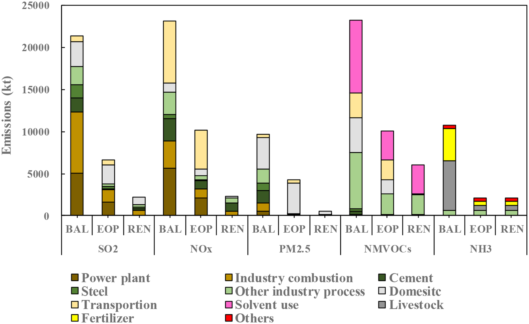
The potential analysis of emission reduction from sectors
The emission of SO2, NOx, primary PM2.5, NMVOCs and NH3 will decrease by 69.2%, 56.1%, 53.8%, 56.6% and 80.3%, respectively under EOP scenario. Under REN scenario by applying renewable energy, the emission of SO2, NOx, primary PM2.5, and NMVOCs will be 89.7%, 89.9%, 94.6%, and 74.0% lower than those in the BAL scenario. The total abatement potential of SO2, NOx, primary PM2.5, NMVOCs and NH3 in 2014 is estimated as 19.2 Mt, 20.8 Mt, 9.1 Mt, 17.2 Mt and 8.6 Mt, respectively.
For the end-of-pipe control measures, the industry sector, including cement, iron and steel and other industry processes, has the largest abatement nationwide, with SO2, NOx, primary PM2.5 and NMVOCs reduced by 31.7%, 32.5%, 72.5% and 36.5%, respectively. In particular, for cement and steelmaking sectors, the application of advanced technology including SNCR for NOx controls and high efficiency deduster (i.e., HEFF, ESP+HEFF) for PM controls in cement manufacture, as well as the activated carbon adsorption technology for collaborative reduction of SO2 and NOx during iron and steel making, would bring substantial emission reductions. The application of EOP in industry combustion and power plant can reduce the SO2 emissions by 39.5% and 23.3%, and reduce PM2.5 emissions by 16.8% and 9.1%, respectively. The abatement potential of NOx largely comes from EOP controls in power plant (26.7%) and transportation (20.7%). Petroleum industry and solvent use exhibit largest abatement potentials for NMVOCs with 32.5% and 39.2% emission reduction, respectively. The livestock sector will reach the NH3 abatement by 62.2% due to the application of large scale raising and breeding farm.
Table 8 summaries the abatement potential and the total cost of multi-pollutants in each province in China. In this study, different cost values of the same end-of-pipe measures are investigated due to different economy level and the total cost calculated by the average value. Shandong province exhibits the largest abatement potential with SO2, NOx, primary PM2.5 and NMVOCs reduced by 1993.4 kt, 2268.8 kt, 798.0 kt and 1667.4 kt, respectively. Furthermore, Henan province as one of major agricultural province exhibits the largest abatement potential of NH3 with 748.2 kt, followed by Sichuan province and Shandong province. In JJJ region, the abatement ratio of SO2, NOx, primary PM2.5, NMVOCs and NH3 was 85.6%, 89.8%, 94.4%, 71.8%, and 78.1%, respectively. In YRD region, the abatement ratio of SO2, NOx, primary PM2.5, NMVOCs and NH3 was 93.4%, 90.6%, 96.9%, 67.3%, and 79.2%, respectively. In PRD region, the ratio of that was 92.9%, 88.2%, 96.5%, 71.1% and 81.0%, respectively. Compared with JJJ and PRD region, the YRD region has the largest potential abatement emissions of SO2, NOx, and primary PM2.5, which indicated that further reduction needed to be considered in this region.
Table 8.
Potential for reducing emissions and total cost of multi-pollutants with respect to 2014.
| Pollutants | SO2 | NOx | PM2.5 | NMVOCs | NH3c | ||||||||||||||||||||||||
|---|---|---|---|---|---|---|---|---|---|---|---|---|---|---|---|---|---|---|---|---|---|---|---|---|---|---|---|---|---|
| MPRa
kt (%) |
Total Costb | MPR kt (%) |
Total Cost | MPR kt (%) |
Total Cost | MPR kt (%) |
Total Cost | MPR kt (%) |
Total Cost | ||||||||||||||||||||
| low | high | mean | low | high | mean | low | high | mean | low | high | mean | low | high | mean | |||||||||||||||
| Beijing | 55.8 | (79.4) | 0.3 | 0.4 | 0.4 | 173.3 | (89.7) | 8.9 | 9.4 | 9.1 | 34.5 | (85.7) | 0.2 | 0.2 | 0.2 | 233.6 | (68.7) | 4.6 | 9.5 | 7.0 | 26.0 | (63.1) | 0.0 | 1.4 | 1.4 | ||||
| Tianjin | 212.0 | (88.4) | 1.0 | 1.5 | 1.2 | 264.4 | (91.1) | 6.6 | 7.4 | 7.0 | 88.2 | (94.6) | 0.5 | 0.7 | 0.6 | 226.5 | (69.1) | 3.4 | 8.0 | 5.7 | 37.3 | (73.2) | 0.0 | 1.8 | 1.8 | ||||
| Hebei | 729.1 | (85.3) | 3.1 | 4.3 | 3.7 | 1084.3 | (89.5) | 31.6 | 34.4 | 33.0 | 661.7 | (94.9) | 3.6 | 5.2 | 4.4 | 1025.0 | (73.2) | 17.1 | 34.7 | 25.9 | 461.3 | (77.0) | 0.0 | 18.4 | 18.4 | ||||
| Shanxi | 833.6 | (87.9) | 3.8 | 5.1 | 4.4 | 776.9 | (91.2) | 15.7 | 17.9 | 16.8 | 453.7 | (94.4) | 1.9 | 2.6 | 2.3 | 522.1 | (79.9) | 6.6 | 12.4 | 9.5 | 111.4 | (62.5) | 0.0 | 4.5 | 4.5 | ||||
| Neimeng | 945.1 | (85.8) | 4.8 | 6.1 | 5.5 | 1035.3 | (91.7) | 15.8 | 18.8 | 17.3 | 347.3 | (87.4) | 2.5 | 3.1 | 2.8 | 459.2 | (76.2) | 6.4 | 13.3 | 9.8 | 312.1 | (77.3) | 0.0 | 9.9 | 9.9 | ||||
| Liaoning | 754.2 | (89.9) | 2.7 | 5.6 | 4.1 | 914.1 | (91.2) | 17.4 | 21.0 | 19.2 | 377.3 | (96.6) | 2.3 | 3.2 | 2.7 | 731.4 | (70.3) | 8.5 | 24.7 | 16.6 | 288.0 | (80.1) | 0.0 | 13.5 | 13.5 | ||||
| Jilin | 324.8 | (90.5) | 1.2 | 1.9 | 1.6 | 500.1 | (91.3) | 9.3 | 11.0 | 10.2 | 248.2 | (95.8) | 1.5 | 1.8 | 1.6 | 331.2 | (76.2) | 5.5 | 13.0 | 9.2 | 233.7 | (80.3) | 0.0 | 8.9 | 8.9 | ||||
| Heilongjiang | 255.0 | (90.0) | 1.1 | 1.9 | 1.5 | 585.5 | (91.6) | 11.2 | 13.1 | 12.2 | 287.1 | (93.2) | 2.3 | 2.4 | 2.3 | 418.3 | (78.4) | 6.7 | 17.0 | 11.8 | 273.3 | (78.8) | 0.0 | 10.8 | 10.8 | ||||
| Shanghai | 453.5 | (89.5) | 1.6 | 4.3 | 2.9 | 283.7 | (91.7) | 6.9 | 7.9 | 7.4 | 77.6 | (93.7) | 0.3 | 0.7 | 0.5 | 438.5 | (62.8) | 3.2 | 14.7 | 8.9 | 19.2 | (63.1) | 0.0 | 1.1 | 1.1 | ||||
| Jiangsu | 900.6 | (93.3) | 3.6 | 5.0 | 4.3 | 1170.1 | (90.1) | 28.0 | 30.7 | 29.4 | 461.8 | (97.4) | 4.2 | 5.3 | 4.7 | 1371.9 | (70.2) | 19.6 | 52.8 | 36.2 | 403.7 | (78.1) | 0.0 | 13.9 | 13.9 | ||||
| Zhejiang | 1079.4 | (95.2) | 3.9 | 5.1 | 4.5 | 835.4 | (91.0) | 20.1 | 21.9 | 21.0 | 226.6 | (96.9) | 2.2 | 2.6 | 2.4 | 1114.5 | (65.7) | 12.9 | 40.0 | 26.4 | 148.9 | (75.7) | 0.0 | 7.3 | 7.3 | ||||
| Anhui | 529.6 | (91.8) | 1.6 | 2.7 | 2.2 | 946.4 | (91.6) | 25.4 | 27.7 | 26.6 | 431.9 | (97.7) | 3.9 | 4.5 | 4.2 | 784.3 | (82.2) | 13.7 | 33.8 | 23.8 | 329.0 | (77.7) | 0.0 | 13.9 | 13.9 | ||||
| Fujian | 448.1 | (93.1) | 1.6 | 2.3 | 1.9 | 622.0 | (86.8) | 9.7 | 12.0 | 10.8 | 170.7 | (96.0) | 1.6 | 1.9 | 1.7 | 473.2 | (69.7) | 6.0 | 16.7 | 11.3 | 178.3 | (79.7) | 0.0 | 8.6 | 8.6 | ||||
| Jiangxi | 344.4 | (90.8) | 1.0 | 1.6 | 1.3 | 471.9 | (86.8) | 9.3 | 10.6 | 10.0 | 222.0 | (96.6) | 1.9 | 2.4 | 2.2 | 354.1 | (75.6) | 6.3 | 13.3 | 9.8 | 242.3 | (80.0) | 0.0 | 14.4 | 14.4 | ||||
| Shandong | 1993.4 | (90.4) | 7.8 | 10.8 | 9.3 | 2168.8 | (91.3) | 41.5 | 48.4 | 45.0 | 798.0 | (95.3) | 4.7 | 5.9 | 5.3 | 1667.4 | (70.7) | 26.5 | 60.3 | 43.4 | 579.2 | (76.7) | 0.0 | 24.4 | 24.4 | ||||
| Henan | 837.9 | (90.0) | 3.0 | 4.2 | 3.6 | 1458.2 | (90.8) | 32.8 | 36.6 | 34.7 | 660.6 | (95.4) | 4.4 | 5.2 | 4.8 | 1033.6 | (77.7) | 18.9 | 40.5 | 29.7 | 748.2 | (78.9) | 0.0 | 30.7 | 30.7 | ||||
| Hubei | 971.8 | (87.4) | 3.6 | 6.0 | 4.8 | 858.3 | (87.8) | 17.6 | 20.6 | 19.1 | 470.0 | (92.8) | 3.4 | 4.0 | 3.7 | 710.7 | (76.9) | 10.0 | 25.7 | 17.9 | 440.5 | (76.7) | 0.0 | 19.9 | 19.9 | ||||
| Hunan | 683.6 | (87.5) | 2.5 | 3.7 | 3.1 | 667.6 | (87.3) | 14.1 | 16.1 | 15.1 | 325.1 | (91.1) | 2.9 | 3.4 | 3.1 | 512.6 | (74.0) | 8.6 | 19.0 | 13.8 | 471.6 | (81.4) | 0.0 | 26.9 | 26.9 | ||||
| Guangdong | 885.4 | (92.9) | 3.5 | 5.1 | 4.3 | 1253.5 | (88.2) | 27.2 | 31.2 | 29.2 | 357.4 | (96.5) | 3.3 | 3.8 | 3.5 | 1182.8 | (71.1) | 18.8 | 43.7 | 31.2 | 350.6 | (78.5) | 0.0 | 16.6 | 16.6 | ||||
| Guangxi | 571.4 | (91.3) | 2.0 | 2.8 | 2.4 | 493.5 | (87.7) | 10.0 | 11.5 | 10.7 | 319.6 | (96.9) | 2.6 | 3.0 | 2.8 | 506.0 | (77.5) | 11.1 | 22.4 | 16.8 | 322.3 | (81.0) | 0.0 | 16.0 | 16.0 | ||||
| Hainan | 71.7 | (95.2) | 0.2 | 0.3 | 0.3 | 97.9 | (89.3) | 1.7 | 2.0 | 1.8 | 28.6 | (96.7) | 0.4 | 0.4 | 0.4 | 96.0 | (70.7) | 1.4 | 3.7 | 2.5 | 56.8 | (77.1) | 0.0 | 2.7 | 2.7 | ||||
| Chongqing | 816.4 | (87.3) | 3.4 | 4.6 | 4.0 | 393.1 | (88.0) | 8.9 | 10.1 | 9.5 | 186.2 | (93.4) | 1.7 | 1.9 | 1.8 | 311.0 | (79.3) | 4.7 | 12.5 | 8.6 | 203.7 | (78.7) | 0.0 | 9.6 | 9.6 | ||||
| Sichuan | 1388.6 | (90.1) | 5.1 | 7.6 | 6.3 | 848.4 | (87.4) | 16.3 | 19.3 | 17.8 | 522.6 | (97.4) | 4.8 | 5.4 | 5.1 | 1002.0 | (83.2) | 17.0 | 45.1 | 31.0 | 714.5 | (80.2) | 0.0 | 35.1 | 35.1 | ||||
| Guizhou | 856.7 | (84.1) | 3.9 | 5.0 | 4.4 | 500.1 | (87.3) | 7.6 | 9.0 | 8.3 | 313.9 | (87.1) | 3.0 | 3.3 | 3.2 | 301.5 | (84.2) | 4.7 | 9.7 | 7.2 | 202.0 | (72.9) | 0.0 | 9.2 | 9.2 | ||||
| Yunnan | 375.9 | (87.9) | 1.0 | 1.7 | 1.4 | 438.8 | (87.9) | 9.4 | 10.5 | 9.9 | 240.3 | (93.0) | 2.2 | 2.6 | 2.4 | 334.3 | (80.5) | 6.7 | 12.3 | 9.5 | 393.8 | (80.2) | 0.0 | 17.3 | 17.3 | ||||
| Xizang | 3.3 | (92.8) | 0.0 | 0.0 | 0.0 | 22.1 | (94.1) | 0.8 | 0.8 | 0.8 | 6.0 | (98.1) | 0.1 | 0.1 | 0.1 | 13.0 | (88.2) | 0.5 | 0.7 | 0.6 | 70.9 | (78.9) | 0.0 | 2.6 | 2.6 | ||||
| Shaanxi | 622.2 | (87.9) | 2.9 | 3.5 | 3.2 | 592.0 | (89.7) | 11.5 | 13.0 | 12.3 | 301.1 | (95.0) | 2.5 | 2.9 | 2.7 | 430.4 | (78.5) | 6.0 | 13.4 | 9.7 | 210.2 | (76.3) | 0.0 | 6.4 | 6.4 | ||||
| Gansu | 247.4 | (88.8) | 0.9 | 1.5 | 1.2 | 320.6 | (88.9) | 8.6 | 9.3 | 8.9 | 166.7 | (93.8) | 1.4 | 1.7 | 1.5 | 206.9 | (80.7) | 3.8 | 7.5 | 5.7 | 158.0 | (76.8) | 0.0 | 5.6 | 5.6 | ||||
| Qinghai | 42.6 | (88.5) | 0.1 | 0.3 | 0.2 | 97.7 | (88.5) | 2.1 | 2.4 | 2.2 | 43.9 | (91.9) | 0.4 | 0.4 | 0.4 | 46.2 | (81.0) | 0.9 | 1.6 | 1.3 | 65.6 | (76.8) | 0.0 | 2.6 | 2.6 | ||||
| Ningxia | 238.0 | (93.9) | 1.1 | 1.4 | 1.2 | 190.4 | (91.5) | 3.5 | 4.0 | 3.8 | 80.1 | (97.2) | 0.4 | 0.6 | 0.5 | 71.3 | (79.7) | 1.3 | 2.2 | 1.7 | 46.0 | (74.7) | 0.0 | 1.2 | 1.2 | ||||
| Xinjiang | 721.3 | (93.9) | 2.7 | 3.9 | 3.3 | 696.3 | (93.5) | 9.6 | 11.8 | 10.7 | 209.1 | (95.5) | 1.4 | 1.8 | 1.6 | 272.5 | (76.6) | 4.2 | 8.5 | 6.3 | 260.7 | (76.8) | 0.0 | 6.5 | 6.5 | ||||
| Total | 19192.9 | (89.7) | 75.0 | 110.0 | 92.5 | 20760.5 | (89.9) | 439.0 | 500.4 | 469.7 | 9117.6 | (94.6) | 68.3 | 83.0 | 75.7 | 17181.9 | (74.0) | 265.5 | 632.4 | 449.0 | 8359.3 | (78.0) | 0.0 | 361.8 | 361.8 | ||||
MPR: Maximum potential reduction emissions, unit: kt; (%) represents the reduction ratio to that in 2014.
Total Cost: Calculated by average cost and the range of cost is in supplementary information, unit: billion;
NH3: the low cost of ammonia is zero for uncontrolled in China at present.
Identifying the key province and sector which exhibits the largest potential of air pollutant is useful for policymaker to design effective control policy. From our analysis, the provinces of Shandong, Hebei, Henan and Sichuan show the largest abatement potential for SO2, NOx and primary PM2.5. For NMVOCs controls, the regions of YRD have the substantial abatement potential. Compared to power plant and industry combustion sector, the cement, steelmaking and other industry process (e.g., oil refining, glassmaking and chemical industry) exhibits larger abatement potential to reduce emissions.
4.2. Estimation of marginal abatement cost curves
Figure 2 displays the total marginal abatement cost of five pollutants in China. Both end-of-pipe measures and energy structure adjustment were applied in the development of marginal abatement cost curves. In summary, the total cost of five major air pollutants is up to 1448.6 billion CNY, in which 801.5 billion CNY for EOP scenario (see detail in Table S6). Under REN scenario, the abatement cost of NOx and NMVOCs is much higher than SO2 and PM2.5, about 5 to 6 times high, which is up to 469.7 billion and 449.0 billion CNY compared with SO2 of 92.5 billion, PM2.5 of 75.7 billion CNY and NH3 of 361.8 billion CNY, respectively. The total cost for SO2, NOx and primary PM2.5, and NMVOCs under REN scenario is 2.2, 4.8, 1.8, 1.8 times higher than that of EOP scenario, respectively. High NOx and NMVOCs cost is associated with the lower removal percent and utilization rates with higher marginal abatement cost for denitrification and NMVOCs extraction.
Figure 2.

The marginal abatement cost of multi-pollutants in China
For SO2 controls, the marginal abatement cost curve increases sharply when the reduction ratio reaches 10% and 83%, respectively. The low efficiency end-of-pipe measures in power plant, including turning off some power plants with installed capacity less than 100 MW, were replaced by high-efficiency FGD technology when the reduction ration reach 10%. After that of 83%, the raise of marginal abatement cost curve depended on the higher unit cost of FGD by using nature gas and liquefied petroleum gas (LPG) of boilers and domestic stoves. Furthermore, the application of energy structure adjustment by replacing fossil fuel with wind or solar energy could further reduce SO2 emission, which indicated the renewables may be a cost-effective solution in the future.
For NOx, three turning points appeared as the rising of the marginal abatement cost curve. When the reduction ratio is less than 58.0%, the LNB+SCR technologies and energy structure adjustment were mainly applied in power plant, industry combustion, and domestic. After that, the marginal cost increases sharply with higher cost of activated carbon absorbing method used in sintering process or the SCR technology in gas-fired or oil-fired boilers and domestic stoves. Then, the large-scale upgrade the quality of gasoline product and promote new energy electric vehicle policy, which resulted in the further abatement of NOx after the reduction ration of 77.1%.
For primary PM2.5, when the reduction ratio was larger than 29.3%, the substitution of renewables in coal-fired power plant were more expensive than conventional technologies (i.e., ESP, FF, ESP+FF) as depicted in the cost curve of PM2.5. The dedusting in gas-fired or oil-fired boilers was difficultly and costly of the reduction ratio over 90.5%.
For NMVOCs, the production process of synthetic material, painting, chemical industry, plant oil extraction and solvent use of NMVOCs showed large potential abatement and marginal cost with the reduction ratio of 42.6% to 62.0%. When the reduction ratio was larger than 62.0%, the marginal cost was up to 267.3 billion because of implementation of new energy electric vehicle policy. The urea substitution was used in fertilizer application that the reduction ratio under 38.4% is costly for removing ammonia. Meanwhile it demonstrated there exit larger potential abatement and marginal cost of NH3 in livestock if the reduction ratio exceeded 40%.
Hence, the further reduction of air pollutants should depend on the adjustment of energy structure in our country, e.g., increase of renewable energy generation proportion, closure of high-emission plants, which cause significant social marginal benefit.
Figure 3 shows the abatement potential emissions and cost in different sectors. Industry combustion exhibits the most abatement potential of SO2 with 35.0% in all sectors, which also has the highest abatement cost of 34.4% (31.9 billion CNY). For SO2, the power plant and domestic sectors still exit the larger abatement potential and higher cost. However, the industry process sector, including cement, iron and steel and other industry process, not only has the larger abatement potential (24.5%) but has the lower abatement cost which account for 14.9 billion CNY (16.2%). Compared to power plant and industry combustion, the controls of cement, steelmaking and other industry process are more cost-effective. Similarly, the potential reduction emission of NOx in industry process was 4209 kt (20.3% in total potential abatement emission) with cost of 35.2 billion (7.5% in total cost). About 69.5% abatement cost of NOx is from transportation sector due to the high technology cost and new energy vehicles. For primary PM2.5, the most economically abatement sector is other industry process with 0.1% abatement cost, i.e., lime production, building ceramic production, glass and brick production, which has the abatement potential with 1624 kt. With the largest abatement potential of PM2.5 (3388 kt) in domestic, the total cost was 31.1 billion CNY. For NMVOCs control, solvent use, other industry process, domestic and transportation sectors have the higher abatement potential and cost resulted from disordered management of control and high investment costs. Up to 25.6% NMVOCs could be reduced in other industry process sector, e.g., car manufacturing, vehicle refinishing, and it has the 18.0% of abatement cost (80.9 billion CNY). According to research (He et al., 2018), electric vehicles is a cost-effective way to alleviate air pollution from a life cycle perspective, which point out electric vehicles could reduce VOCs and NOx emission by 1770 to 2354 g/year per vehicle and 930 to 1354 g/year per vehicle, respectively. Especially, the reduction potential of VOCs emissions for vehicle material cycle mainly focus on vehicle fluids (i.e., windshield washer fluid) and vehicle manufacturing (notably the painting process). The maximum potential reduction of NH3 in livestock and fertilizer application were 5352 kt and 3254 kt with the total cost of 347.7 billion and 14.1 billion, respectively. The unit cost of NH3 in livestock was the highest in all sectors which indicated it was more difficult and expensive for reducing NH3 in livestock.
Figure 3.

The abatement potential and total cost by sector
4.3. Relationship between abatement cost and local economy
We also investigated the relationship of unit abatement costs and local economy at provincial level, as displayed in Figure 4. The R was the ratio of GDP at each province to the nationwide in 2014. The larger the R value, the higher the ratio of GDP. The slope represents the unit cost of abated emissions (purple line represents the national level). Generally, the total abatement cost increases along with the total abatement potential. However, differences in slope are still noticeable among provinces.
Figure 4.

The unit costs of abated air pollutants at provincial level with local economy.
For SO2, two kinds of regions exhibit cost-effective reduction emissions, which one represented high GDP with intensive industries (i.e., Zhejiang, Shandong) and another represented lower GDP with high sulfur content of coal for reduction SO2 emissions (i.e., Sichuan). The better quality of coal with low sulfur constant results in the higher unit cost of abatement emissions in Inner Mongolia which are the main coal mining and renewable energy supply areas as explained in previous studies (Dong et al., 2015). Meanwhile, the less cost-effective regions were Beijing, Tianjin, and Shanghai, which showed relatively lower potential reduction. That is because the end-of-pipe measures has been fully implement in those developed eastern regions and the unit cost raised for further reduction which highly depended on renewable energy application.
For NOx, the cost-effective reduction regions were Inner Mongolia, Xinjiang, and Guizhou province. The least cost-effective regions are located in the provinces with high potential abatement, high population density and vehicle population, including Beijing, Shandong, Henan, Hebei, Guangdong, Jiangsu, Anhui, and Zhejiang.
For primary PM2.5, Shandong, Henan, and Hebei provinces exhibit huge potential abatement and high cost to control. The most cost-effective region was Shanxi, while the least cost-effective regions included Hainan, Xizang, and Qinghai.
For NMVOCs, there was higher potential abatement and total cost in developed areas, such as Shandong, Jiangsu, Guangdong, Sichuan, Henan, and Zhejiang province.
For NH3, the potential abatement regions included some major agricultural provinces, such as Sichuan, Henan, Hunan, and Shandong. In summary, it is important to pay more attention to regional disparity with different economic levels and energy structures for policy making to improve the whole air quality.
5. Conclusion
This study investigated the abatement potential and cost of multi-pollutants in China, by implementing local dataset which reflect the fact of actual operating conditions, including investment cost, fixed operating and maintenance cost, removal percent and application rate of end-of-pipe control technologies.
The result shows that the total maximum abatement potentials of SO2, NOx, primary PM2.5, NMVOCs and NH3 in China are 19.2 Mt, 20.8 Mt, 9.1 Mt, 17.2 Mt and 8.6 Mt, respectively, based on the emission level of 2014. For the end-of-pipe control measures, the industry sector, including cement, iron and steel and other industry process (i.e., oil refining, glassmaking and chemical industry), still has the largest abatement nationwide. The SO2, NOx, primary PM2.5 and NMVOCs can be reduced by 31.7%, 32.5%, 72.5% and 36.5%, respectively after the application of end-of-pipe control measures. Compared to other regions, Shandong province has the most abatement potential with SO2, NOx, PM2.5 and NMVOCs accounting for 1993.4 kt, 2168.8 kt, 798.0 kt and 1667.4 kt respectively, followed by Sichuan, Hebei, and Henan provinces.
Application of renewable energy can further reduce the pollutants but with much more cost from end-of-pipe controls. Results suggest that the emission of SO2, NOx, PM2.5, and NMVOCs will be further decreased by 89.7%, 89.9%, 94.6%, and 74.0% under REN scenario based on 2014 emission level. The marginal abatement cost of air pollutants in China, including applications of both end-of-pipe measures and renewable energy application, is 92.5 billion of SO2, 469.7 billion of NOx, 75.7 billion of primary PM2.5, 449.0 billion of NMVOCs, and 361.8 billion of NH3, respectively. Comparing the limitation of conventional EOP technologies, the application of renewable energy to replace fossil fuel could result in further reduction of pollutants, which illustrated the renewable energy application can be another option besides end-of-pipe measures in the future.
Different control measures are suggested to be implemented based on local industry structure and economy level. For SO2 and NOx, the end-of-pipe technologies employed in industry process (i.e., lime production, building ceramic production, glass and brick production) were more cost-effective than that of in fossil fuel sectors (i.e., power plant, industry combustion, domestic). The application of renewable energy could significantly increase the marginal abatement cost for further reduction especially for SO2 and NOx. For PM2.5, the total cost in cement was still larger than other sectors, suggesting implement more stringent end-of-pipe controls. However, the end-of-pipe technology, as a matter of priority, still can be a cost-efficiency way to control NMVOCs and NH3 which have huge abatement potential in China.
The discrepancy in the economic level among provinces are also recommended to be taken into consideration when designing control policy. Provinces with higher potential abatement emissions and total abatement costs are those developed regions with higher GDP, such as Shandong, Jiangsu, Henan, Zhejiang, and Guangdong. However, the least-effective regions with high GDP, including Beijing, Shanghai, and Tianjin, have limited potential reduction due to the high unit abated cost.
In general, this study gathered most available local information about marginal abatement cost, the application rate of control measures, and further calculated the corresponding emission abatement and associated costs in China. These abatement potential analysis and costs assessment will contribute to the analysis with integrated assessment model (e.g., ABaCAS) to design cost-effective control strategies for policymakers to improve air quality. The marginal abatement cost curves developed in this study can also be used by combining with air quality model simulation, to further evaluate the cost-effectiveness of abatement policy designed to achieve certain ambient air quality target.
Supplementary Material
Acknowledgment
This work was supported in part by National Science Foundation of China (51861135102), National Key R & D program of China (2017YFC0210006), National Research Program for Key Issues in Air Pollution Control (DQGG0301), National Key R & D program of China (2017YFC0213005), and National Key Technology R&D Program (2014BAC06B05). This work was completed on the “Explorer 100” cluster system of Tsinghua National Laboratory for Information Science and Technology.
Reference
- Eyth Alison, Del Vecchio Darin and Yang D (2008). Recent Applications of the Control Strategy Tool (CoST) within the Emissions Modeling Framework. 17th Annual Emissions Inventory Conference. Portland. [Google Scholar]
- Amann M, Bertok I, Borken-Kleefeld J, Cofala J, et al. , (2011). “Cost-effective control of air quality and greenhouse gases in Europe: Modeling and policy applications.” Environmental Modelling & Software 26(12): 1489–1501. [Google Scholar]
- Amann M, Johansson M, Lükewille A, Schöpp W, et al. , (2001). “An integrated assessment model for fine particulate matter in Europe.” Water, Air, and Soil Pollution 130(1–4): 223–228. [Google Scholar]
- Amann M, Kejun J, Jiming HAO, Wang S, et al. , (2008). GAINS Asia:Scenarios for cost-effective control of air pollution and greenhouse gases in China. Sixth Framework Program (FP6) of the European Union Report. Laxenburg, Austria, IIASA. [Google Scholar]
- Bollen J, van der Zwaan B, Brink C and Eerens H (2009). “Local air pollution and global climate change: A combined cost-benefit analysis.” Resource and Energy Economics 31(3): 161–181. [Google Scholar]
- Buonocore JJ, Luckow P, Norris G, Spengler JD, et al. , (2015). “Health and climate benefits of different energy-efficiency and renewable energy choices.” Nature Climate Change 6(1): 100–105. [Google Scholar]
- Burke M, Davis WM and Diffenbaugh NS (2018). “Large potential reduction in economic damages under UN mitigation targets.” Nature 557(7706): 549–553. [DOI] [PubMed] [Google Scholar]
- Chestnut LG and Mills DM (2005). “A fresh look at the benefits and costs of the US acid rain program.” J Environ Manage 77(3): 252–266. [DOI] [PubMed] [Google Scholar]
- Cofala J, Amann M, Gyarfas F, Schoepp W, et al. , (2004). “Cost-effective control of SO2 emissions in Asia.” Journal of Environmental Management 72(3): 149–161. [DOI] [PubMed] [Google Scholar]
- Dong L, Dong H, Fujita T, Geng Y, et al. , (2015). “Cost-effectiveness analysis of China’s Sulfur dioxide control strategy at the regional level: regional disparity, inequity and future challenges.” Journal of Cleaner Production 90: 345–359. [Google Scholar]
- ERINDRC (2015). China 2050 High Renewable Energy Penetration Scenario and Roadmap Study, Energy Research Institute of National Development and Reform Commission, Beijng, China. [Google Scholar]
- Fu X, Wang S, Zhao B, Xing J, et al. , (2013). “Emission inventory of primary pollutants and chemical speciation in 2010 for the Yangtze River Delta region, China.” Atmospheric Environment 70: 39–50. [Google Scholar]
- Heo J, Adams PJ and Gao HO (2016). “Public Health Costs of Primary PM2.5 and Inorganic PM2.5 Precursor Emissions in the United States.” Environ Sci Technol 50(11): 6061–6070. [DOI] [PubMed] [Google Scholar]
- Hill J, Polasky S, Nelson E, Tilman D, et al. , (2009). “Climate change and health costs of air emissions from biofuels and gasoline.” Proc Natl Acad Sci U S A 106(6): 2077–2082. [DOI] [PMC free article] [PubMed] [Google Scholar]
- Hu X, Jiang K and Yang H (2003). Application of AIM/Enduse model to China. Climate Policy Assessment, Springer: 75–91. [Google Scholar]
- Huang K, Fu JS, Gao Y, Dong X, et al. , (2014). “Role of sectoral and multi-pollutant emission control strategies in improving atmospheric visibility in the Yangtze River Delta, China.” Environ Pollut 184: 426–434. [DOI] [PubMed] [Google Scholar]
- IRENA (2015). Renewable power generation costs in 2014. Amin AZ, The International Renewable Energy Agency. [Google Scholar]
- Kanada M, Dong L, Fujita T, Fujii M, et al. , (2013). “Regional disparity and cost-effective SO2 pollution control in China: A case study in 5 mega-cities.” Energy Policy 61: 1322–1331. [Google Scholar]
- Klimont Z, Cofala J, Bertok I, Amann M, et al. , (2002). Modeling Particulate Emissions in Europe. A framework to estimate reduction potential and control costs. IIASA Interim Report. Laxenburg, Austria, IIASA. IR-11–027. [Google Scholar]
- Klimont Z and Winiwarter W (2011). Integrated ammonia abatement -Modelling of emission control potentials and costs in GAINS. IIASA Interim Report. Laxenburg, Austria, IIASA. IR-11–027. [Google Scholar]
- Liu F, Klimont Z, Zhang Q, Cofala J, et al. , (2013). “Integrating mitigation of air pollutants and greenhouse gases in Chinese cities: development of GAINS-City model for Beijing.” Journal of Cleaner Production 58: 25–33. [Google Scholar]
- Loughlin DH, Macpherson AJ, Kaufman KR and Keaveny BN (2017). “Marginal abatement cost curve for nitrogen oxides incorporating controls, renewable electricity, energy efficiency, and fuel switching.” J Air Waste Manag Assoc 67(10): 1115–1125. [DOI] [PMC free article] [PubMed] [Google Scholar]
- Lu X, Yao T, Fung JC and Lin C (2016). “Estimation of health and economic costs of air pollution over the Pearl River Delta region in China.” Sci Total Environ 566–567: 134–143. [DOI] [PubMed] [Google Scholar]
- MEE (2012). Emission standard of air pollutants for cement industry. E. S. Institute, Ministry of Ecology and Environment of the People’s Republic of China. [Google Scholar]
- MEE (2016). Limits and measurement methods for emissions from light-duty vehicles(CHINA 6). GB18352.6—2016. E. S. Institute, Ministry of Ecology and Environment of the People’s Republic of China. [Google Scholar]
- Millstein D, Wiser R, Bolinger M and Barbose G (2017). “The climate and air-quality benefits of wind and solar power in the United States.” Nature Energy 2(9): 17134. [Google Scholar]
- Shi Minjun, Xiang Nan and Li N (2017). Policy assessment report of air pollution management in Beijing -Tianjin-Heibei. Renmin University of China, National Academy of development and strategy. [Google Scholar]
- NBS (2013). China statistical yearbook, China Statistics Press Beijing. [Google Scholar]
- NBS (2015). China statistical yearbook, China Statistics Press Beijing. [Google Scholar]
- Pearce D (1998). “cost benefit analysis and environmental policy.” Oxford review of economic policy 14(4): 84–100. [Google Scholar]
- Schopp W, Amann M, Cofala J, Heyes C, et al. , (1999). “Integrated assessment of European air pollution emission control strategies “ Environmental Modelling & Software 14(1999): 1–9. [Google Scholar]
- Sun J, Schreifels J, Wang J, Fu JS, et al. , (2014). “Cost estimate of multi-pollutant abatement from the power sector in the Yangtze River Delta region of China.” Energy Policy 69: 478–488. [Google Scholar]
- van Donkelaar A, Martin RV, Brauer M and Boys BL (2015). “Use of satellite observations for long-term exposure assessment of global concentrations of fine particulate matter.” Environ Health Perspect 123(2): 135–143. [DOI] [PMC free article] [PubMed] [Google Scholar]
- Wang J, Xing J, Mathur R, Pleim JE, et al. , (2016). “Historical Trends in PM2.5-Related Premature Mortality during 1990–2010 across the Northern Hemisphere.” Environ Health Perspect 125(3): 400–408. [DOI] [PMC free article] [PubMed] [Google Scholar]
- Wang J, Zhao B, Wang S, Yang F, et al. , (2017). “Particulate matter pollution over China and the effects of control policies.” Sci Total Environ 584–585: 426–447. [DOI] [PubMed] [Google Scholar]
- Wang S, Nan J, Shi C, Fu Q, et al. , (2015). “Atmospheric ammonia and its impacts on regional air quality over the megacity of Shanghai, China.” Scientific Reports 5: 15842. [DOI] [PMC free article] [PubMed] [Google Scholar]
- Wang S, Xing J, Chatani S, Hao J, et al. , (2011). “Verification of anthropogenic emissions of China by satellite and ground observations.” Atmospheric Environment 45(35): 6347–6358. [Google Scholar]
- Wang SX, Zhao B, Cai SY, Klimont Z, et al. , (2014). “Emission trends and mitigation options for air pollutants in East Asia.” Atmospheric Chemistry and Physics 14(13): 6571–6603. [Google Scholar]
- Wei W, Wang S, Chatani S, Klimont Z, et al. , (2008). “Emission and speciation of non-methane volatile organic compounds from anthropogenic sources in China.” Atmospheric Environment 42(20): 4976–4988. [Google Scholar]
- Wei W, Wang S, Hao J and Cheng S (2011). “Projection of anthropogenic volatile organic compounds (VOCs) emissions in China for the period 2010–2020.” Atmospheric Environment 45(38): 6863–6871. [Google Scholar]
- Xing J, Wang S, Jang C, Zhu Y, et al. , (2017). “ABaCAS: an overview of the air pollution control cost-benefit and attainment assessment system and its application in China.” The Magazine for Environmental Managers–Air & Waste Management Association. [Google Scholar]
- Xing R, Hanaoka T, Kanamori Y, Dai H, et al. , (2015). “An impact assessment of sustainable technologies for the Chinese urban residential sector at provincial level.” Environmental Research Letters 10(6): 065001. [Google Scholar]
- Zhang J, Zhang Y.-x., Yang H, Zheng C.-h., et al. , (2017). “Cost-effectiveness optimization for SO 2 emissions control from coal-fired power plants on a national scale: A case study in China.” Journal of Cleaner Production 165: 1005–1012. [Google Scholar]
- Zhang S, Worrell E and Crijns-Graus W (2015). “Evaluating co-benefits of energy efficiency and air pollution abatement in China’s cement industry.” Applied Energy 147: 192–213. [Google Scholar]
- Zhao B, Jiang JH, Diner DJ, Su H, et al. , (2018). “Intra-annual variations of regional aerosol optical depth, vertical distribution, and particle types from multiple satellite and ground-based observational datasets.” Atmospheric Chemistry and Physics 18(15): 11247–11260. [DOI] [PMC free article] [PubMed] [Google Scholar]
- Zhao B, Wu W, Wang S, Xing J, et al. , (2017). “A modeling study of the nonlinear response of fine particles to air pollutant emissions in the Beijing–Tianjin–Hebei region.” Atmospheric Chemistry and Physics 17(19): 12031–12050. [Google Scholar]
- Zhao B, Xu J and Hao J (2011). “Impact of energy structure adjustment on air quality: a case study in Beijing, China.” Frontiers of Environmental Science & Engineering in China 5(3): 378–390. [Google Scholar]
- Zheng H, Cai S, Wang S, Zhao B, et al. , (2018). “Development of a unit-based industrial emission inventory in the Beijing-Tianjin-Hebei region and resulting improvement in air quality modeling.” Atmospheric Chemistry and Physics Discussions: 1–24. [Google Scholar]
Associated Data
This section collects any data citations, data availability statements, or supplementary materials included in this article.