Abstract
This work proposes a novel framework for brain tumor segmentation prediction in longitudinal multi-modal MRI scans, comprising two methods; feature fusion and joint label fusion (JLF). The first method fuses stochastic multi-resolution texture features with tumor cell density feature to obtain tumor segmentation predictions in follow-up timepoints using data from baseline pre-operative timepoint. The cell density feature is obtained by solving the 3D reaction-diffusion equation for biophysical tumor growth modelling using the Lattice-Boltzmann method. The second method utilizes JLF to combine segmentation labels obtained from (i) the stochastic texture feature-based and Random Forest (RF)-based tumor segmentation method; and (ii) another state-of-the-art tumor growth and segmentation method, known as boosted Glioma Image Segmentation and Registration (GLISTRboost, or GB). We quantitatively evaluate both proposed methods using the Dice Similarity Coefficient (DSC) in longitudinal scans of 9 patients from the public BraTS 2015 multi-institutional dataset. The evaluation results for the feature-based fusion method show improved tumor segmentation prediction for the whole tumor(DSCWT = 0.314, p = 0.1502), tumor core (DSCTC = 0.332, p = 0.0002), and enhancing tumor (DSCET = 0.448, p = 0.0002) regions. The feature-based fusion shows some improvement on tumor prediction of longitudinal brain tumor tracking, whereas the JLF offers statistically significant improvement on the actual segmentation of WT and ET (DSCWT = 0.85 ± 0.055, DSCET = 0.837 ± 0.074), and also improves the results of GB. The novelty of this work is two-fold: (a) exploit tumor cell density as a feature to predict brain tumor segmentation, using a stochastic multi-resolution RF-based method, and (b) improve the performance of another successful tumor segmentation method, GB, by fusing with the RF-based segmentation labels.
Keywords: Tumor segmentation prediction, Longitudinal MRI, Feature and label fusion, Reaction-diffusion equation, Lattice-Boltzmann method, Texture features, BraTS
1. Introduction
Brain tumors may be classified as benign or malignant based on grade, and primary or metastatic based on origin. According to the World Health Organization (WHO) diagnostic schema [1], tumors of the central nervous system (CNS) may be graded as I, II, III, and IV, based on multiple factors including similarity of tumor cells to normal cells, growth rate, presence of definitive tumor margins, and vascularity. Among these classes, grade III tumor contains actively reproducing abnormal cells that infiltrate between adjacent cells, and grade IV tumors are the most malignant with rapid proliferation and infiltration to surrounding tissues [2,3]. In 2016, WHO suggested a new CNS tumor classification schema, based on both phenotype and genotype expressions in addition to growth pattern and behaviors [4]. Glioblastoma (formerly glioblastoma multiforme, GBM) is the most common and deadly among all human primary CNS tumors [5], with extensive heterogeneity radiographically reflected by various sub-regions, comprising enhancing (ET) and non-enhancing tumor (NET), as well as peritumorally edematous/invaded tissue (ED). GBM originates from glial cells and grows by infiltrating surrounding tissues. Even though there have been many treatment advancements, the median overall survival period of patients diagnosed with GBM still remains 12–16 months [5].
Brain tumor detection, segmentation, and tracking its changes over time (henceforth, tumor segmentation prediction) is of particular importance for diagnosis, treatment planning, patient management, and monitoring. In practice, manual tumor segmentation by radiologists is tedious, time-consuming and prone to human error. Longitudinal brain tumor segmentation is a critically challenging task due to the tumor’s unpredictable appearance, infiltration to surrounding tissue, intensity heterogeneity, size, shape, and location variation [6]. There are many brain tumor segmentation techniques published in the literature. Active contour methodologies have been used for both image recognition tasks [7], as well as brain tumor segmentation tasks [8,9], to identify in single 2D MRI slices the boundary of the whole tumor extent as a single region. However, they cannot be considered directly applicable for the task of our study, which attempts to identify multiple tumor sub-regions in 3D, within the whole tumor extent, while utilizing multiple MRI modalities. Gooya et al. introduced a generative approach for registering a probabilistic atlas of a healthy population to brain MRI scans with glioma and simultaneously segmenting these scans into tumor and healthy tissue labels [10,11]. Cuadra et al. proposed an atlas-based segmentation of pathological brain MRI scans using a lesion growth model [12]. Bauer et al. also introduced an atlas-based segmentation of brain tumor images using a Markov random field-based tumor growth model and non-rigid registration [13]. However, these atlas-registration based techniques may be tedious and error prone, since they require accurate deformable image registration of tumor bearing slices with the atlas.
To avoid the issues with image registration, other studies consider the brain tumor segmentation as a feature-based classification problem [14,15]. The general idea of feature-based methods is to extract features and provide them to a classifier, to learn the most representative of the class(es) in question, and hence obtain segmentation labels in new unseen cases. Islam et al. extracted sophisticated texture features among others and applied the AdaBoost algorithm to segment tumors [16]. Reza et al. proposed an improved texture feature based multiple abnormal brain tissue classification method using Random Forest (RF) [17,18]. SVM has also been used as a classifier for brain tumor segmentation [19]. In addition, others have utilized super-pixels to classify tumor tissue. Wang et al. used a graph-based segmentation technique to over-segment images into homogeneous regions [20,21]. Pei et al. applied simple linear iterative clustering (SLIC) to obtain super-pixel [22]. Kadkhodaei et al. applied a semi-supervised ‘tumor-cut’ method to over-segment images [23]. The super-pixel-based segmentation relies on the quality of the approach used for the over-segmentation. Finally, over recent years, various approaches based on CNN have been used for brain tumor segmentation [14,24,25]. However, to the best of our knowledge, the tumor cell density pattern has not been used as a feature in tumor segmentation prediction by others. The cell density feature can be obtained from solving the biophysical tumor growth modeling such that to predict potential tumor development in the future.
Longitudinal brain tumor segmentation prediction is not only related to the accurate segmentation of the various tumor sub-regions, but also reveals information about the tumor development over time. Monitoring longitudinal brain tumor changes is useful for follow-up of treatment-related changes, assessment of treatment response and guiding dynamically changing treatments, including surgery, radiation therapy and chemotherapy. Fig. 1 shows a longitudinal brain tumor example for a patient from BraTS 2015 patient dataset [6]. This figure shows that enhancing, necrosis and other surrounding tissues of the tumor for an example patient in timepoint 2 are evolving (increasing) during the elapsed time by comparing that of timepoint 1.
Fig. 1.
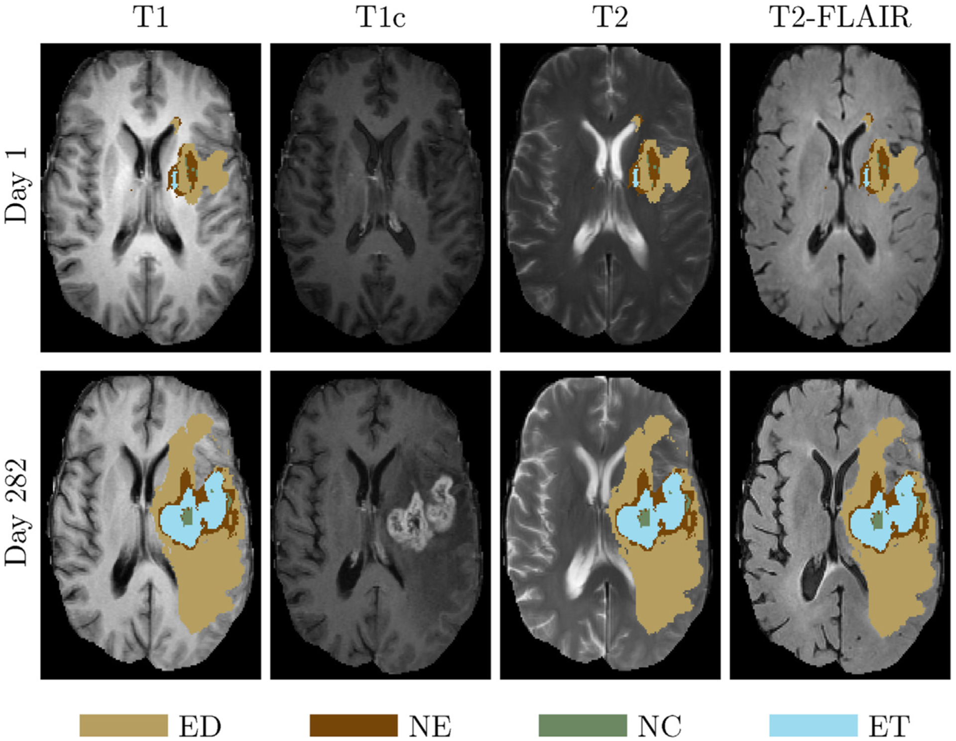
A longitudinal brain tumor example. Top from left to right: T1 overlaid with GT, T1c, T2 overlaid with GT, T2-FLAIR overlaid with GT at timepoint 1. Bottom shows the corresponding images overlaid with GT at timepoint 2 (282 days after timepoint 1).
To model and predict the growth of a tumor, a reaction-diffusion equation is generally employed [11,26–30]. Hu et al. simulated one-dimensional tumor growth based on logistic models [31]. Sallemi et al. simulated brain tumor growth based on cellular automata and fast marching method [32]. However, none of these methods explicitly obtains tumor segmentation using growth patterns as features. Clatz et al. proposed a GBM tumor growth simulation by solving reaction-diffusion equation using finite element method [33]. Xu et al. used phase fields to model cellular growth, and reaction-diffusion equations for the dynamics of angiogenic factors and nutrients [34]. We have recently proposed a novel feature, which assesses temporal changes of tumor cell density, based on biophysical tumor growth modeling, for segmentation prediction [22]. Meier et al. used a fully automatic segmentation method for longitudinal brain tumor volumetry [35]. However, Meier’s work only focuses on analyzing each timepoint independently, and does not include a setting to integrate knowledge from prior timepoints for longitudinal tumor study.
Here we propose a novel longitudinal brain tumor segmentation prediction, using two different fusion approaches: a feature-fusion approach, where unique tumor growth-based cell density and texture features are used, and a label-fusion, where segmentation labels obtained from two state-of-the-art tumor growth and stochastic texture models are utilized. In the feature-fusion-based segmentation prediction method, we build upon a stochastic multiresolution texture model [17] to obtain cell density information from tumor growth patterns as novel features and then fuse them with texture features. The tumor growth model is based on a reaction-diffusion equation that is solved in 3D using a Lattice-Boltzmann method (LBM), a class of computational fluid dynamics method for fluid simulation. On the other hand, the proposed joint label-fusion (JLF) method fuses segmentation labels obtained from a hybrid generative-discriminative brain tumor segmentation method that incorporates a biophysical tumor growth model [36,37] and the stochastic tumor segmentation models [16–18], to achieve tumor segmentation predictions. For traditional multi-label fusion, multiple target images are registered and weighted by comparing a target image to multiple atlas images. Further, the reference labels are obtained by considering tissue labels from registering the target image to the atlas images. In this study, due to the presence of multiple tumors in the provided MRI volumes, we did not use healthy atlases as reference images, but instead created consensus average images across all patients for each MRI modality. The reference labels are obtained by the RF and the GB segmentation models. The fusion weight is obtained proportional to the inverse of intensity difference by target images to reference images.
The overall novelty of this work is two-fold: (a) the tumor cell density is used as a novel feature to obtain tumor growth segmentation prediction for a prior successful stochastic multiresolution RF-based segmentation method, and (b) it obtains improved tumor segmentation performance of another successful tumor segmentation tool, GB, by fusing labels obtained from with the RF-based tumor segmentation method.
The remaining sections are organized as follows: Section 2 introduces the related background, including texture-based tumor segmentation, biophysical tumor growth modeling, and JLF. Section 3 discusses proposed methods in the paper, whereas Section 4 describes the algorithm used in the paper. Finally, Section 5 discusses the experiments and results, and conclusions are discussed in Section 6.
2. Background
In this section, we discuss texture-based tumor segmentation, tumor growth modeling, and JLF.
2.1. Multi-fractal Brownian Motion (mBm) process and feature extraction
The mBm is a non-stationary zero-mean Gaussian random process that corresponds to the generalization of fractional Brownian motion (fBm) [18]. The fBm considers a rough heterogeneous appearance of tumor texture in brain MRI. In the fBm process, the local degree of Hurst index (H) is a constant. The value of H determines the randomness of the fBm process. However, tumor texture in MRI may appear as a multifractal structure that is a time (t) and/or space varying process and is represented by mBm. The mBm process is defined as x(at) = aH(t)x(t), where x(t) is the mBm process with a scaling factor, a, and the time varying Hurst index H(t). The mBm features effectively model spatially varying heterogeneous tumor texture. Its derivation combines the multi-resolution analysis enabling one to capture spatially varying random inhomogeneous tumor texture at different scales [16]. More details for these multiscale texture features and their efficacy in brain tumor segmentation can be found in [16–18].
2.2. Random Forest classification
Random Forest (RF) is an ensemble learning method that can be used for classification, regression, and segmentation [38]. Classification based on RF, has been heavily used in the medical image analysis domain due to its very fast, and efficient multi-class handling capability [17,39].
Consider n samples and feature vectors with outcomes yi, then the data are represented as D = {(v1, y1), …, (vn, yn)}. The feature vector (v) of a sample (i) is represented by vi = (vi1, …, vid), where d denotes the dimensionality of the feature vector. A classification tree is a decision tree in which each node has a binary decision based on whether vi is less than a threshold a. At each node, feature vid and threshold a are chosen to minimize resulting ‘diversity’ in the children nodes that are measured by the Gini criterion [38]. Ensemble of classifiers h = {h1 (v), …, hk(v)}, and we define parameters of the decision tree for each classifier hk(x) to be θk = (θk1, θk2, …, θkp). We can write: hk(v) = h(v|θk). A Random Forest is a classifier based on a family of classifiers {h(v|θk), k = 1, 2, …, K} with parameters θk, which are randomly chosen from a model random vector θ.
In RF classification, given a fixed ensemble h = {h1(v), …, hk(v)}, where v is a random vector and K is the number of trees in the forest, the estimated probability for predicting class c for a sample set, is defined as:
| (1) |
where pt(c|v) is the estimated density of class labels at the tth tree. The final multi-class decision function of the forest is defined as:
| (2) |
The generalization error (GE) has an upper bound in form of:
| (3) |
where is the mean correlation between pairs of trees in the forest, and s is the strength of the set of classifiers.
2.3. Biophysical tumor growth model
Tumor growth describes an abnormal growth of tissue, which usually involves cell proliferation, invasion, and mass effect to the tumor surrounding tissues. During cell invasion, tumor cells migrate as a cohesive and multicellular group with retained cell–cell junctions and penetrate to surrounding healthy tissues. Tissues in the brain may deform due to mass effect. Biophysical tumor growth modeling simulates the interactive process occurring between the abnormal tissue (i.e., tumor) and the surrounding brain tissues, and parameterizes the collective changes in the brain, including death, infiltration to surrounding tissues, and proliferation. The reaction-diffusion equation has been widely used to model brain tumor growth [28–31], using a diffusion and a logistic proliferation term given as:
| (4) |
and
| (5) |
where ns is the tumor cell density, D is the diffusion coefficient while infiltrating, and ρ is the proliferation rate. Eq. (5) enforces Neumann boundary conditions on the brain domain Ω, and is unit normal vector on the ∂Ω pointing inward to the domain.
2.4. Joint label fusion
Joint label fusion (JLF) has been developed in recent years and used for analysis medical images [20,21]. Compared to the single-atlas based method, multi-atlas based label fusion reduces errors associated with any single atlas propagation in the process of combination, and the weight for each atlas is computed independently. However, different atlases may produce similar label errors. To solve this issue, Wang et al. proposed an advanced multi-atlas label fusion, known as joint label fusion [40]. Multi-atlas label fusion enforces co-registration with sample images to target image and minimizes independent errors to improve the segmentation result [41]. In general, the label map is computed by using the following equation:
| (6) |
where is the ith training image, and ϕi is the transfer function during image registration. l is the candidate label map of the testing image I. JLF () achieves consensus segmentation as,
| (7) |
where ωx(i) is the individual voting weight of ith reference, and is the probability that x votes for label l of the i-th reference. The weight is determined by,
| (8) |
where 1n = [1 ; 1 ; …, 1] is a vector of size n and Mx(i) is the pairwise dependency matrix that estimates the likelihood of two references both producing wrong segmentations on a per-voxel basis for the target images.
For the ith reference, the dependency matrix is computed as:
| (9) |
where m indices correspond to all modality channels, and is the vector of absolute intensity difference between a selected reference image and the target image over local patches υ centered at voxel j and x, respectively. 〈 · , · 〉 is the dot product. LM is the total number of modalities [40].
3. Materials and methods
This study proposes two distinct methods for longitudinal brain tumor segmentation prediction: a feature-based and JLF-based. Application of the proposed methods, assumes appropriate preprocessing of the provided multimodal MRI brain scans, consisting of noise reduction, bias field correction, scale standardization, and histogram matching.
3.1. Data
The brain tumor scans used to quantitatively evaluate the proposed methods in this study belong to retrospective longitudinal multi-institutional cohorts of patients diagnosed with GBM, from the publicly available Multimodal BRAin Tumor Segmentation (BraTS 2015) challenge dataset [6]. Nine patients with longitudinal multimodal MRI (mMRI) scans with growing tumors along time were chosen from the BraTS 2015 dataset. The brain scans for each patient consist of four MRI modalities, namely native T1-weighted (T1), contrast-enhanced T1-weighted (T1c), T2-weighted (T2), and T2 Fluid-attenuated inversion recovery (T2-FLAIR).
Note that we use the BraTS 2015 dataset instead of the latest BraTS 2018 dataset [6,37,42,43], as the latter provides only pre-operative mMRI scans, whereas the BraTS 2015 data describes paired combinations of pre- and post-surgical mMRI brain scans for each patient, with isotropic (1 mm3) resolution images of size 240 × 240 × 155. The manually evaluated ground truth labels of these brain scans were also available, allowing for the quantitative validation of the proposed methods. These ground truth labels delineate the tumor sub-regions of necrotic/fluid-filled core (NC), non-enhancing/solid tumor (NE/ET), edema (ED), and everything else grouped together, with labels of 1, 3, 4, 2, and 0, respectively. In this study, we apply the proposed method to the nine longitudinal patient data from BraTS 2015.
3.2. Pre-processing
MRI scans are known to be significantly affected by numerous acquisition artifacts, such as intensity non-uniformities, which are caused by the inhomogeneity of the scanner’s magnetic field during image acquisition (also known as bias field), and Gaussian noise. These factors degrade the MRI quality significantly [44], potentially affecting the accuracy of automated segmentation of various tissue regions, as well as the image registration process. Therefore, preprocessing is an essential step for MRI analysis that includes several steps, such as skull-stripping (also known as brain extraction), noise reduction, bias field correction, and co-registration across modalities. The BraTS brain scans used in this study were already co-registered and skull-stripped. We corrected for the appearing bias field using N4ITK [45].
3.3. Feature fusion based method
The method proposed in this study utilizes tumor growth patterns as novel features to improve texture-based tumor segmentation in longitudinal MRI. The proposed pipeline is shown in Fig. 2.
Fig. 2.
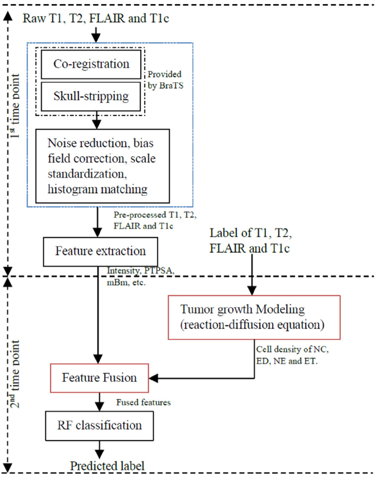
Pipeline of the proposed method. At the 1st scan date, we extract texture (e.g., fractal, and mBm) and intensity features, and obtain the ground truth label map for different brain tissues from baseline pre-operative (i.e., first timepoint) mMRI scans. The ground truth at this first timepoint is used to obtain the tumor growth modeling and enable to predict cell density for the next timepoint. Finally, considering the cell density pattern as a new feature, we fuse it with other features using a RF classifier to generate the label of the second timepoint.
By using proposed feature-based fusion, the random vector v is defined as:
| (10) |
and the label of target image is defined as:
| (11) |
where c is the candidate label of target image. K is the number of the tree applied. v is a feature vector. θt is the classifier parameter obtained from training process and pt is the classification probability of label c by giving feature v at tth tree, respectively. FD describes the mBm feature. ns is the tumor cell density derived by tumor growth model (Eq. (4)). Ipre and Ipost are the image intensities before and after intensity normalization (scale standardization [46]), respectively. Hist is the intensity histogram of all modality images (T1, T1c, T2, and T2-FLAIR).
Two feature types were used in the proposed method, representing local and spatial descriptors. Local features comprise the intensity of each modality before and after scaling standardization, as well as after histogram matching, their pairwise intensity differences among image modalities, and the cerebrospinal fluid (CSF) mask, obtained by the CSF expected intensity across modalities. Spatial features include a fractal feature extracted from multi-modal MRI, named piecewise-Triangular Prism Surface Area (PTPSA), the mBm features that combine both multiresolution-fractal and wavelet analyses for each modality after scaling standardization, and 6 Gabor-like Texton features.
3.4. Joint label fusion based method
Label fusion has been successfully used for tumor segmentation in recent years [40,41]. The method proposed here employs JLF for improving tumor segmentation prediction by fusing stochastic feature-based tumor labels, with segmentation labels obtained from a hybrid generative-discriminative brain tumor segmentation method that incorporates a biophysical tumor growth model, namely GLISTRboost [36,37,47]. Our proposed pipeline is shown in Fig. 3. Initially, GB is applied on the 2nd timepoint in parallel with independent application of the RF-based approach, and their output segmentation labels are then fused together leading to the consensus result.
Fig. 3.
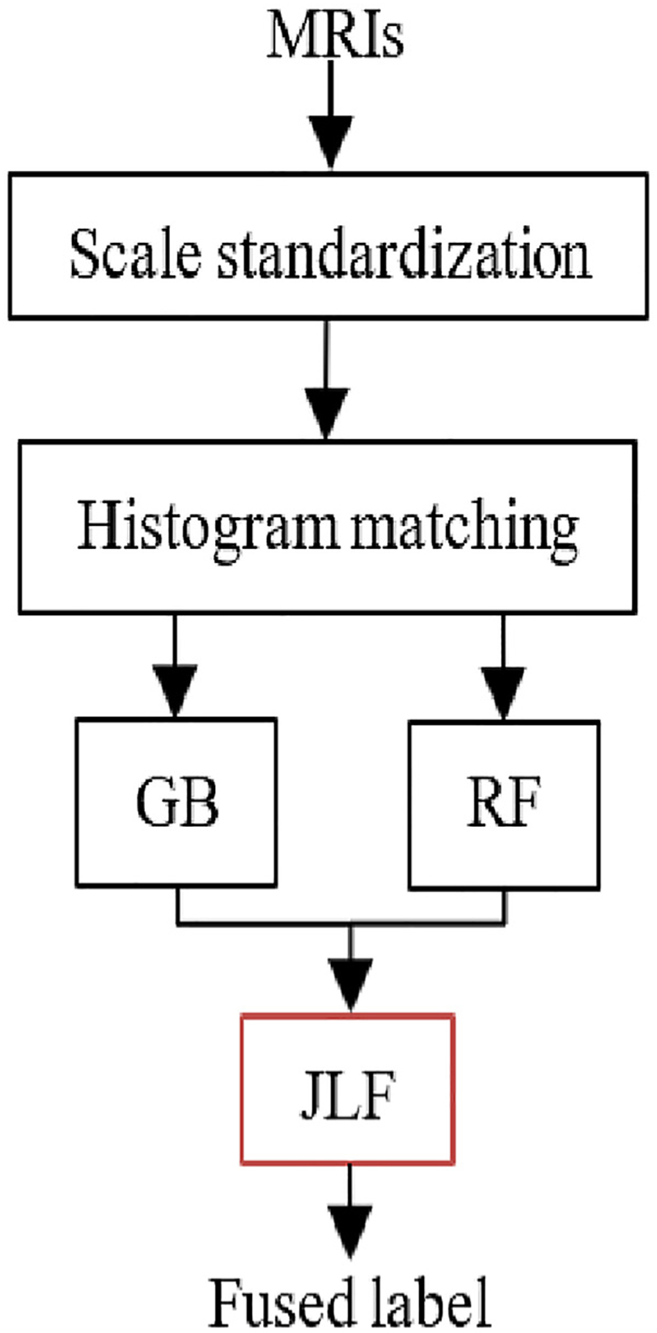
Pipeline for joint label fusion based tumor segmentation prediction.
All provided MRI scans were affinely co-registered to an atlas template [48] and skull-stripped by BraTS. We then scaled all modality intensities for one reference subject to the range [0–255] and then matched the histograms of each modality across all subjects. The error dependence matrix (Eq. (9)) was then computed between the target and the reference image, which describes the consensus average images across all patients. By using the error dependency matrix, we calculate the voting weight (Eq. (8)), and finally the agreement label (Eq. (7)) is obtained.
In GB, the probabilities of ET and NE are defined as:
| (12) |
where Y is observation set, Φ is the intensity distribution, h is the reference domain, q is the tumor growth model parameters. πk is the k abnormal tissue, and fk· is a multivariate Gaussian distribution.
Application of the JLF method requires all four provided MRI volumes (T1, T1c, T2, and FLAIR), the label map LGB obtained by GB (Eq. (12)) and the segmentation result LRF obtained by Eqs. (1) and (2). Specifically, in order to use the JLF, the voting weights are obtained by computing the error dependency matrix from all the available modalities to the reference images (Eq. (8)). For calculating the dependency matrix (Eq. (9)). υ(x) is a 5 × 5 ×5 patch centered at location x. Am(m ∈ {1, 2, 3, 4}) describes the volumes T1, T1c, T2, and T2-FLAIR of the training images, respectively. Tm is the target image. A is the reference image including the GB segmentation (AGB) and RF classification (ARF). The candidate labels at location x for either the GB or the RF segmentations are defined as:
| (13) |
Let’s define Dirac delta function δ(l|x) as 1, if the predicted label is the same as the reference label, otherwise 0, then, Eq. (13) becomes:
| (14) |
where the dependency matrix of M is computed by using Eq. (9). In the special case of the images among references being the same, , then Eq. (14) will be simplified as a majority voting: p(l|x) = 0.5 (δGB(l|x) + δRF(l|x)). Therefore, it is recommended to choose an odd number of templates.
3.5. Lattice-Boltzmann method for tumor growth modeling
To solve the reaction-diffusion in Eq. (4), different methods such as finite element method (FEM) [26] and Lattice-Boltzmann method (LBM) [30] may be used. We use the LBM method for its computational efficiency and easy parallelization. The LBM is defined as [49]:
| (15) |
where is the one particle distribution function of specifies s with velocity at node , at time t. and are non-reactive and active terms, respectively.
| (16) |
where τ is the relaxation time. is the equilibrium distribution function, which depends on and t corresponding to a system with zero mean flow given as:
| (17) |
where ns is the cell density and Λs,i weight depending on the lattice system.
Two-dimensional nine-velocity (D2Q9) model is commonly used in 2D cases. The nine discrete velocities are as follows (Fig. 4).
Fig. 4.
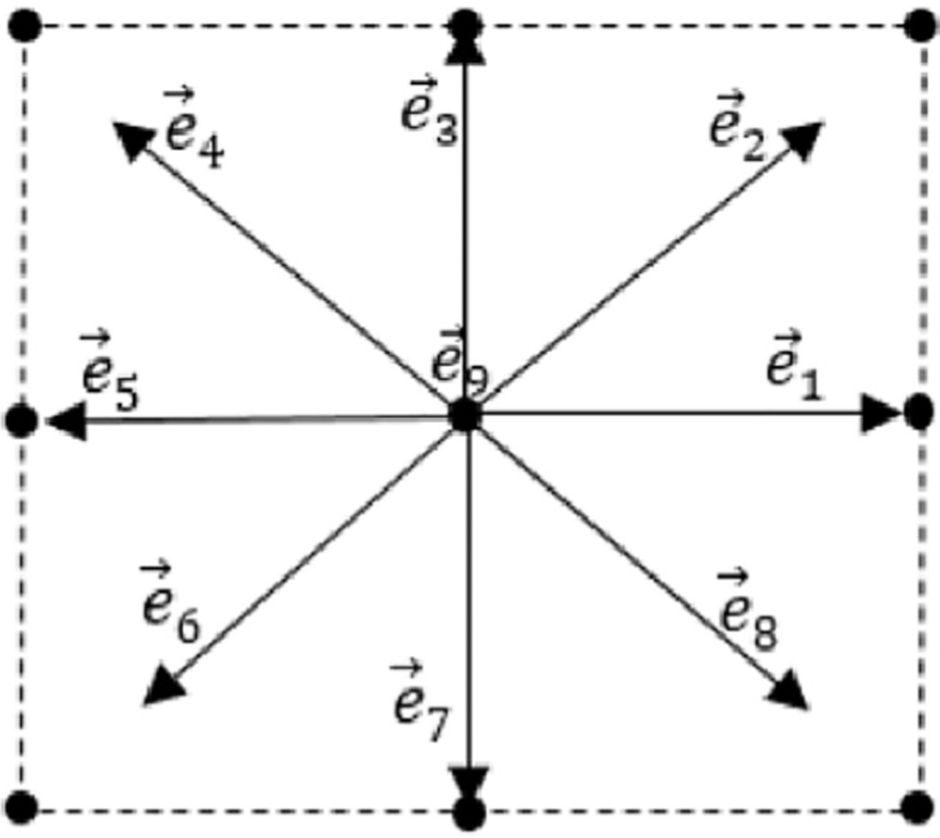
Illustration of a lattice with D2Q9 model.
Let’s define:
| (18) |
Here ns is the cell density as defined in Eq. (1), and Λs,i is defined as:
| (19) |
By using LBM, the reaction-diffusion equation (Eq. (4)) can be recovered as:
| (20) |
| (21) |
Setting offers solution for Eq. (4).
The algorithm of the proposed method is listed in Algorithm 1.
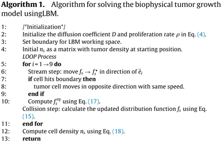
3.6. Longitudinal tumor segmentation prediction
By longitudinal tumor segmentation prediction, we refer to the accurate delineation of the tumor boundaries in any follow up time-point, given the segmentation of the tumor in the first scan. This does not only allow for the segmentation of the tumor but it also reveals information about its longitudinal growth and aggressiveness/behavior.
For feature fusion-based method, we build a tumor growth model by solving the reaction-diffusion equation using LBM. Diffusion coefficient D and proliferation rate ρ are important parameters to simulate tumor growth using the model. To predict tissues growth using the model, the parameters of the model are suggested within [0.02, 1.5] mm2/day, and [0.002, 0.2]/day [30]. We empirically set DNC, ρNC as 0.052, 0.01, DED, ρED as 0.06, 0.009, DNE, ρNE as 0.03, 0.014, DET, ρET as 0.05, 0.01 for NC, ED, NE, and ET, respectively. For the JLF method, we integrate a stochastic texture feature-based segmentation with another state-of-the-art, named GLISTRboost (GB) to achieve a better segmentation.
4. Evaluation
4.1. Performance evaluation
In the BraTS dataset, the ground truth is manually annotated by qualified raters, following a hierarchical majority voting rule [6,25]. To quantitatively evaluate the proposed brain tumor segmentation prediction method, a criteria policy is required. Specifically, three different tumor regions are evaluated, as defined by the BraTS challenge [6].
-
Region 1 – Whole tumor (WT)
This region defines the whole tumor (WT), which consists of the union of all tumor labels. Although the ED is a peripheral tissue to the tumor core, it is still considered as part of the WT since it is not pure edema but also includes invaded tumor cells.
-
Region 2 – Tumor core (TC)
This region defines the tumor core (TC), which comprises the combination of NC, NE and ET. Note that the TC describes what is typically resected during surgery.
-
Region 3 – Enhancing tumor (ET)
The ET region biologically represents regions of contrast leakage through disrupted blood-brain barrier.
We evaluate the 3D volume overlap by computing the Dice similarity coefficient [50], where A and B represent the segmentation labels of a given method and the manually annotated (i.e., ground truth) labels. The DSC value ranges in [0, 1], where 0 represents that the two comparing regions do not have any overlap and 1 means that the regions are identical.
5. Experimental results and discussion
5.1. Experiment with feature fusion based method
To solve the biophysical brain tumor growth model using LBM, three parameters need to be considered: diffusion coefficient D, proliferation rate ρ, and simulated days t. The diffusion coefficient and proliferation rate are variable to the model. Choosing a value for these variables is challenging. The value of D is chosen within [0.02, 1.5] mm2/day, ρ ∈ [0.002, 0.2]/day, after considering the available literature [30]. Fig. 5 shows an example of longitudinal tumor growth using the proposed method and as depicted by ground truth labels in a single slice for a patient in the BraTS 2015 dataset.
Fig. 5.
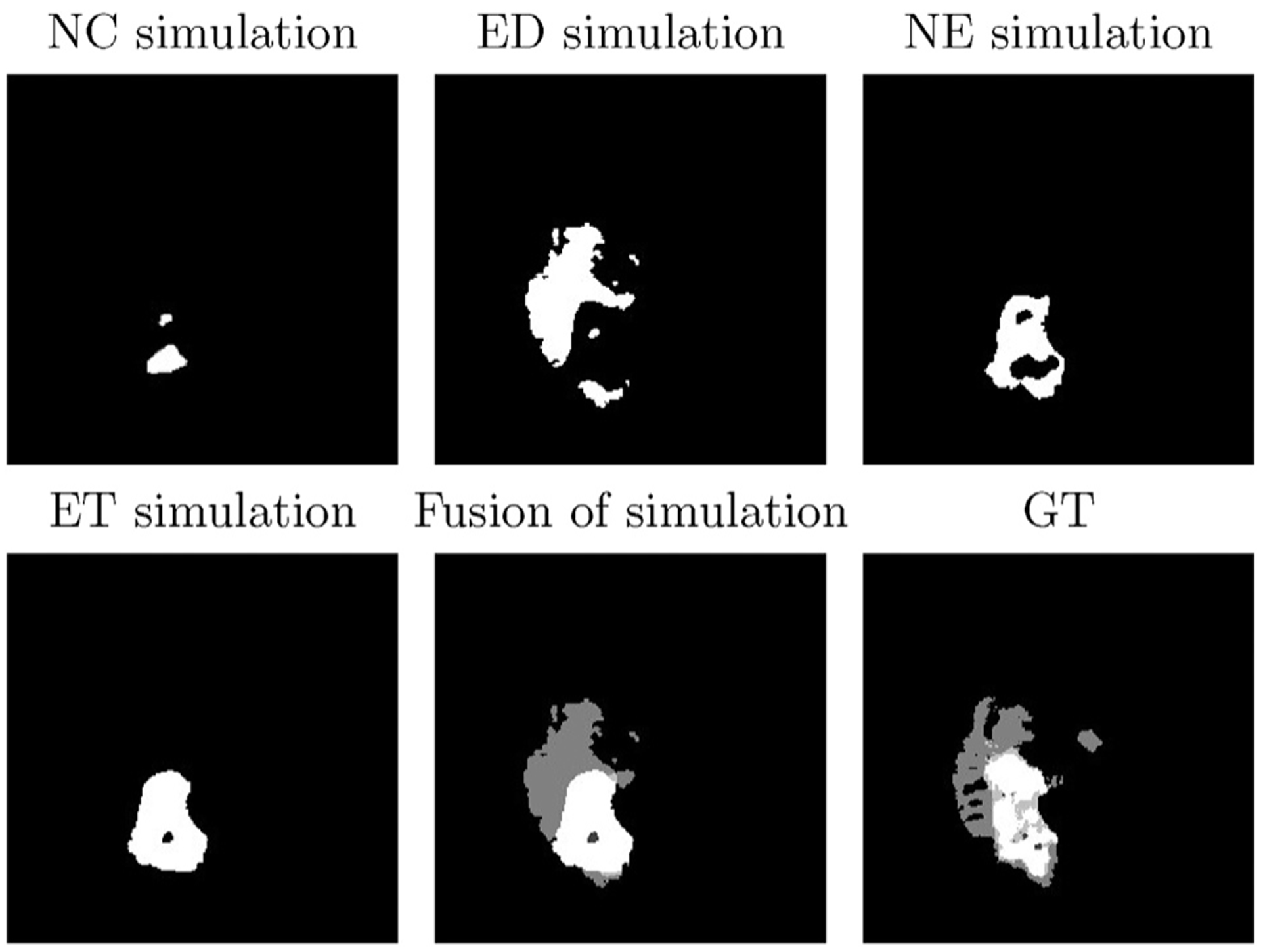
An example of longitudinal tumor growth by using the proposed method for one slice of patient 439. Top row (from left to right): NC simulation with D = 0.052, ρ = 0.01, ED simulation with D = 0.06, ρ = 0.009, and NE simulation with D = 0.03, ρ = 0.014. Bottom row (left to right): ET simulation with D = 0.05, ρ = 0.01, fusion of all simulations, and corresponding GT.
We then apply the tumor growth model to real patient data from the BraTS dataset, where each patient’s scan includes information of all sub-regions, i.e., NC, ED, NE, and ET. We simulate all these abnormal tissues separately, and then fuse them all into the final label map of the patient. Parameters vary among the various tissues [30]. By using the LBM model, we obtain the cell density patterns for the NE, ET and the WT tissues, respectively. Note that the WT comprises all sub-regions including ED and NC. Following previous work [18], we use a total of 30 features (completed features in Appendix A) including fractal, mBm, intensity and intensity difference among MRI modalities. The fractal and mBm are spatial features that capture surface variation.
For specification of (Eq. 11), label c ∈ {0, 1, 2, 3, 4} which represents background, NC, ED, NE and ET, respectively. K is empirically chosen as 20, and number of random feature is 5, which is approximately equal to the square root of total number of features. Addition of cell density as a feature, results in 30 features (density of NC, ED, NE, and ET) extracted from each MRI slice. Fig. 6 gives an illustrative example of comparing two cases between tissue segmentation obtained before and after adding cell density as a feature type for a patient.
Fig. 6.
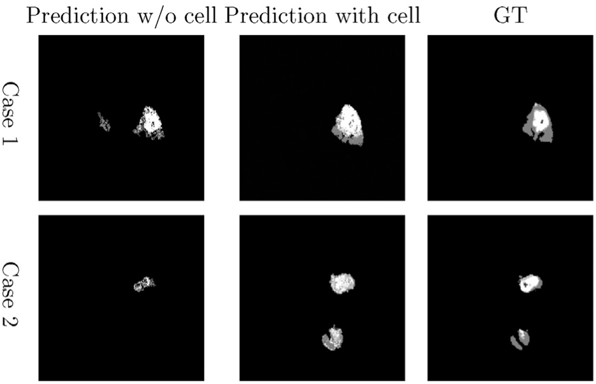
Examples of tumor segmentation prediction by using the proposed method. Left column: Segmentation without cell density feature. Middle column: Segmentation with cell density, and right column: Corresponding ground truth of each patient at second time scan.
We evaluate the performance of the proposed method and compare the DSC to the segmentation prediction without cell density features (Fig. 7). We further evaluate the statistical significance of the obtained results using paired t-test for all patients. The p-values for segmentation prediction obtained with and without inclusion of the cell density feature show statistical significance for WT, TC and ET tissues (Table 1). The paired t-test analysis shows that fusion of tumor growth pattern with texture and intensity features offers a significant improvement in the segmentation prediction of TC and ET tissue regions. However, the statistical analysis does not suggest significant improvement for the WT tissue. We hypothesize that the reason for this is that the WT label, which represents the abnormal T2-FLAIR signal, is well-segmented by the originally applied methods (both GB and RF) and hence there is not substantial significant improvement offered by the proposed method.
Fig. 7.
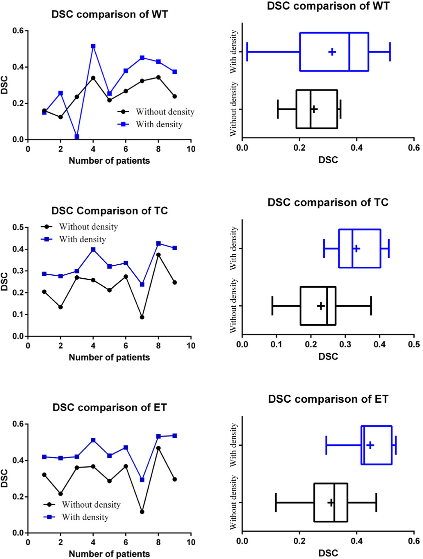
Comparison of tumor growth prediction segmentation using the proposed method. Vertical line and + sign indicate the median and the mean, respectively.
Table 1.
Paired t-test for comparison of volume between w/o and with cell density by using RF to predict the tumor segmentation labels in timepoint 2, using data from timepoint 1.
| DSCWT | DSCTC | DSCET | |
|---|---|---|---|
| Result w/o cell density | 0.251 ±0.08 | 0.229 ±0.08 | 0.311 ± 0.101 |
| Result with cell density | 0.314 ±0.16 | 0.332 ± 0.065 | 0.448 ±0.076 |
| p-Value | 0.150 | 0.0002 | 0.0002 |
5.2. Experiment with joint label fusion-based method
We apply the JLF-based brain tumor segmentation prediction to process data from all nine patients at timepoint 2 (post-op scans). To evaluate the performance, we use a Leave-One-Out cross-validation schema to compute the DSC of segmentations at timepoint 2 from the proposed method and compare to the ground truth and to segmentations generated by GB [36,37] (Fig. 8). An example segmentation prediction result is shown in Fig. 9. From the collective summary of comparisons, we note that the proposed method offers better results than GB alone. The result DSC for the proposed method is 0.850 ± 0.055 for WT, 0.836 ± 0.041 for TC, and 0.837 ± 0.0074 for ET.
Fig. 8.
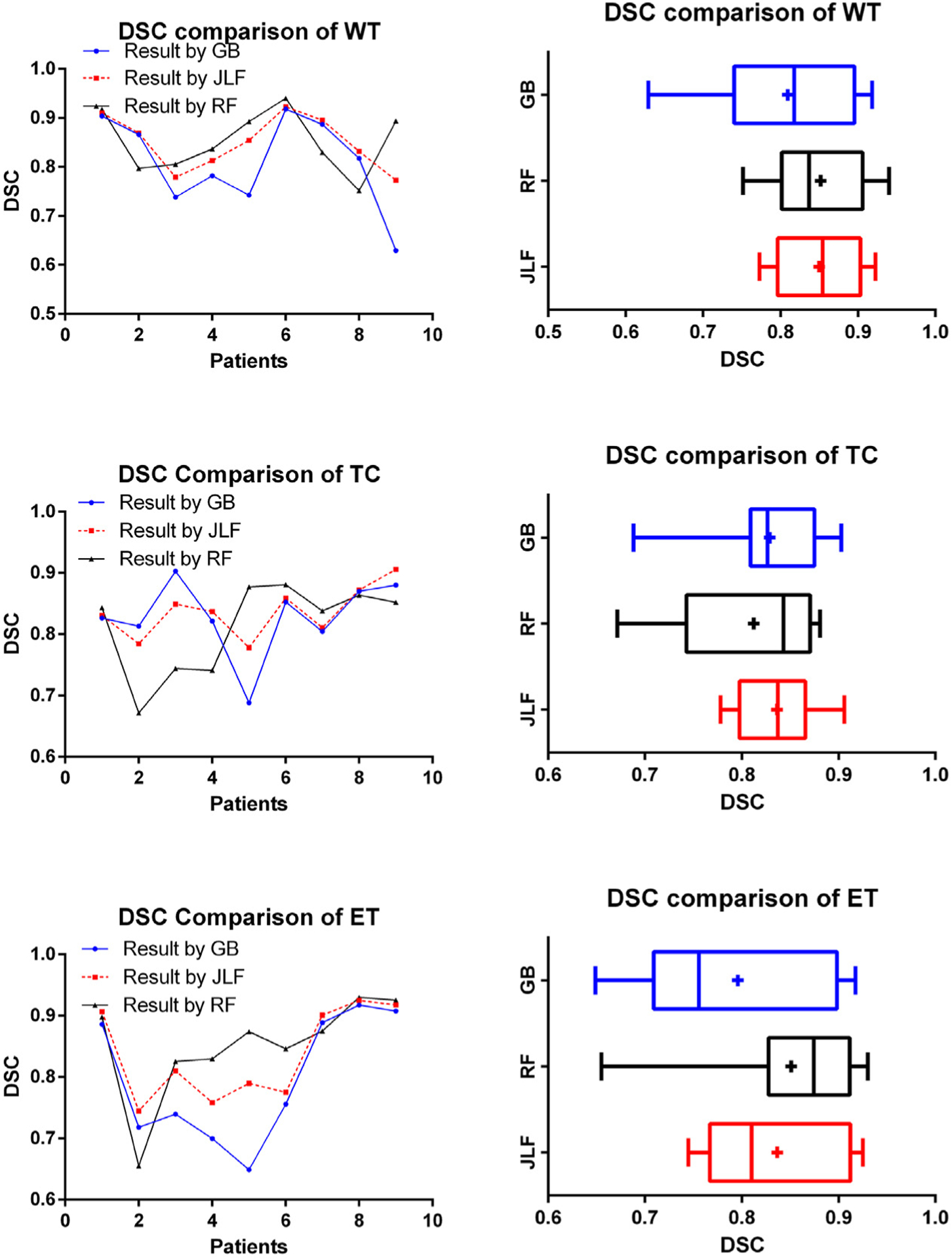
DSC comparison results among GB, RF, and proposed method (JLF). Vertical line and + sign indicate the median and the mean, respectively.
Fig. 9.
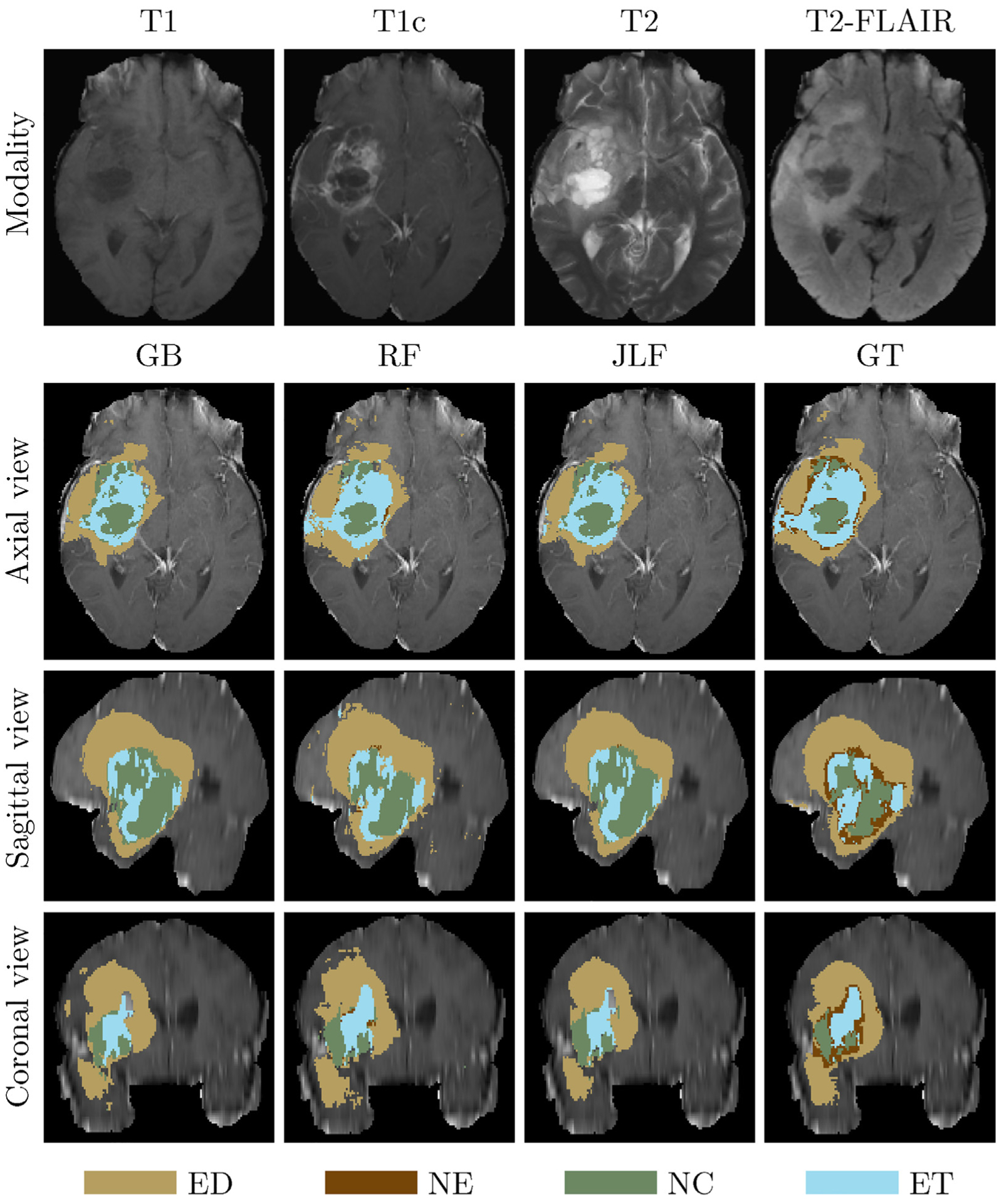
An example of label fusion-based application. The first (top) row denotes the input brain scans. Rows 2–4 illustrate shows the axial, sagittal, and coronal views, respectively, of the T1c input scan overlaid with GB, RF, JLF and GT labels.
We also statistically evaluate the segmentation prediction results using ANOVA and the resulting p-values are shown in Table 2. The JLF method offers statistically significant improvements on tumor segmentation performance for the WT and ET regions, when compared to the results of the GB method. The overall performance is better than GB and RF across all patients, as shown in Fig. 8.
Table 2.
Performance of 3D brain tumor growth prediction segmentation.
| WT | TC | ET | |
|---|---|---|---|
| Ave. DSC by GB | 0.810 ±0.095 | 0.829 ±0.062 | 0.796 ±0.104 |
| Ave. DSC by RF | 0.852 ±0.063 | 0.812 ±0.074 | 0.851 ± 0.093 |
| Ave. DSC by JLF | 0.850 ±0.055 | 0.836 ±0.041 | 0.837 ±0.007 |
| Median DSC by GB | 0.8177 | 0.8266 | 0.7557 |
| Median DSC by RF | 0.8369 | 0.8430 | 0.8743 |
| Median DSC by JLF | 0.8544 | 0.8372 | 0.8100 |
| p-Value (GB,JLF) | 0.047 | 0.579 | 0.023 |
In addition, we also compare the proposed work with BraTumIA (BTIA) [35], a state-of-art tool that has been previously used for brain tumor segmentation in longitudinal scans. We applied BraTumIA to the patient data used in our experiments and the obtained results shown the superiority of our proposed approach (Table 3). Results for all experiments are also given in false positive and false negative rates (Appendix B).
Table 3.
Longitudinal tumor segmentation comparison of average DSC between BraTumIA [35] and JLF.
| DSCWT | DSCTC | DSCET | |
|---|---|---|---|
| BraTumlA [35] | 0.761 ±0.104 | 0.703 ±0.186 | 0.732 ±0.140 |
| JLF | 0.850 ±0.055 | 0.836 ±0.041 | 0.837 ±0.075 |
5.3. Discussion
In this work, we propose two methods for longitudinal brain tumor segmentation prediction, in longitudinal mMRI. Feature fusion using RF and tumor cell density offers improved performance for predicting longitudinal tumor growth. Specifically, this method shows significant prediction improvement of TC and ET abnormal tissues, while these is no significant improvement for WT tissue. On the other hand, the JLF using RF and GB labels shows improvement on WT and ET abnormal tissues over that of the GB labels alone. Note that due to availability of limited number of longitudinal tumor growth patient cases used in this study, the segmentation prediction performance is not optimal for all possible types of abnormal tissue.
6. Conclusion and future work
This work proposes two novel methods for longitudinal brain tumor segmentation prediction: feature fusion-based and joint label fusion-based. The feature fusion-based method offers improved texture-based brain tumor segmentation in longitudinal mMRI by fusing tumor cell density patterns obtained from biophysical tumor growth modeling with the stochastic texture features in a RF-based segmentation method. Statistical analysis shows significant performance improvement for the proposed feature fusion method for the areas of TC and ET. The JLF-based method fuses results obtained from RF with that of GB and helps to improve GB, a state-of-the-art method on longitudinal brain tumor segmentation.
In order to make the proposed framework more useful, we plan to extend the models for segmentation of other abnormal tissues such as cyst and necrosis associated with brain tumor. A more robust label fusion may help for the second method to obtain improved longitudinal tumor segmentation prediction. We further plan to improve the underlying feature extraction, tumor growth and segmentation models. A more comprehensive tumor growth model development that also considers the treatment modalities may be interesting.
Acknowledgements
This work was partially funded through NIH grants by NIBIB, NINDS, and NCI/ITCR, under award numbers R01EB020683, R01NS042645, and U24CA189523, respectively.
Appendix A.
All 30 features used in our proposed method [17].
| 1 | 2 | 3 | 4 | 5 | 6 |
| Intensity of T1 (pre) | PTPSA of T1 | mBm of T1 | Intensity of T2 (pre) | PTPSA of T2 | mBm of T2 |
| 7 | 8 | 9 | 10 | 11 | 12 |
| Intensity of FL (pre) | PTPSA of FL | mBm of FL | Intensity of T1c (pre) | PTPSA of T1c | mBm of T1c |
| 13 | 14 | 15 | 16 | 17 | 18 |
| Texton of T2 (No. 37) | Texton of T2 (No. 38) | Texton of FL (No. 4) | Texton of FL (No. 37) | Texton of FL (No. 38) | Texton of T1c (No. 37) |
| 19 | 20 | 21 | 22 | 23 | 24 |
| Intensity of T1 (post) | Intensity of T2 (post) | Intensity of FL (post) | Intensity of T1c (post) | D21 | D21C |
| 25 | 26 | 27 | 28 | 29 | 30 |
| D2f | Hist. T1 | Hist. T2 | Hist. FL | Hist. T1c | CSF mask |
Note: Note: In the Table, “pre” means before normalization, “post” is after normalization. “FL” represents FLAIR modality, “D21” is the intensity difference between T2 and T1. “D21C” is intensity difference between T2 and TIC, and “D2f” is for intensity difference between T2 and FLAIR. “Hist.” means histogram matched.
Appendix B.
Average false negative rate (FNR) and false positive rate (FPR) comparison between result of the proposed method and BraTumIA (BTIA)
| Tumor type | WT | TC | EN | |||
|---|---|---|---|---|---|---|
| JLF | BTIA | JLF | BTIA | JLF | BTIA | |
| FNR | 0.227 | 0.3426 | 0.2489 | 0.3833 | 0.1159 | 0.2698 |
| FPR | 0.000889 | 0.000956 | 0.000344 | 0.0006 | 0.0009 | 0.000778 |
Footnotes
Declaration of Competing Interest
The authors do not have any conflict of interest for this work.
References
- [1].Louis DN, Ohgaki H, Wiestler OD, Cavenee WK, Burger PC, Jouvet A, Scheithauer BW, Kleihues P, The 2007 who classification of tumours of the central nervous system, Acta Neuropathol. 114 (2) (2007) 97–109. [DOI] [PMC free article] [PubMed] [Google Scholar]
- [2].Hill CI, Nixon CS, Ruehmeier JL, Wolf LM, Brain tumors, Phys. Therapy 82 (5) (2002) 496–502. [PubMed] [Google Scholar]
- [3].Kralik S, Taha A, Kamer A, Cardinal J, Seltman T, Ho C, Diffusion imaging for tumor grading of supratentorial brain tumors in the first year of life, Am. J. Neuroradiol 35 (4) (2014) 815–823. [DOI] [PMC free article] [PubMed] [Google Scholar]
- [4].Louis DN, Perry A, Reifenberger G, von Deimling A, Figarella-Branger D, Cavenee WK, Ohgaki H, Wiestler OD, Kleihues P, Ellison DW, The 2016 world health organization classification of tumors of the central nervous system: a summary, Acta Neuropathol. 131 (6) (2016) 803–820. [DOI] [PubMed] [Google Scholar]
- [5].Chen J, McKay RM, Parada LF, Malignant glioma: lessons from genomics, mouse models, and stem cells, Cell 149 (1) (2012) 36–47. [DOI] [PMC free article] [PubMed] [Google Scholar]
- [6].Menze BH, Jakab A, Bauer S, Kalpathy-Cramer J, Farahani K, Kirby J, Burren Y, Porz N, Slotboom J, Wiest R, et al. , The multimodal brain tumor image segmentation benchmark (brats), IEEE Trans. Med. Imaging 34 (10) (2015) 1993. [DOI] [PMC free article] [PubMed] [Google Scholar]
- [7].Olszewska JI, Active contour based optical character recognition for automated scene understanding, Neurocomputing 161 (2015) 65–71. [Google Scholar]
- [8].Sachdeva J, Kumar V, Gupta I, Khandelwal N, Ahuja CK, A novel content-based active contour model for brain tumor segmentation, Magn. Reson. Imaging 30 (5) (2012) 694–715. [DOI] [PubMed] [Google Scholar]
- [9].Angulakshmi M, Lakshmi Priya G, Automated brain tumour segmentation techniques – a review, Int. J. Imaging Syst. Technol 27 (1) (2017) 66–77. [Google Scholar]
- [10].Gooya A, Biros G, Davatzikos C, Deformable registration of glioma images using em algorithm and diffusion reaction modeling, IEEE Trans. Med. Imaging 30 (2) (2011) 375–390. [DOI] [PMC free article] [PubMed] [Google Scholar]
- [11].Gooya A, Pohl KM, Bilello M, Cirillo L, Biros G, Melhem ER, Davatzikos C, Glistr: glioma image segmentation and registration, IEEE Trans. Med. Imaging 31 (10) (2012) 1941–1954. [DOI] [PMC free article] [PubMed] [Google Scholar]
- [12].Cuadra MB, Pollo C, Bardera A, Cuisenaire O, Villemure J-G, Thiran J-P, Atlas-based segmentation of pathological MR brain images using a model of lesion growth, IEEE Trans. Med. Imaging 23 (10) (2004) 1301–1314. [DOI] [PubMed] [Google Scholar]
- [13].Bauer S, Seiler C, Bardyn T, Buechler P, Reyes M, Atlas-based segmentation of brain tumor images using a markov random field-based tumor growth model and non-rigid registration, in: 2010 Annual International Conference of the IEEE Engineering in Medicine and Biology Society (EMBC), IEEE, 2010, pp. 4080–4083. [DOI] [PubMed] [Google Scholar]
- [14].Pereira S, Pinto A, Alves V, Silva CA, Brain tumor segmentation using convolutional neural networks in MRI images, IEEE Trans. Med. Imaging 35 (5) (2016) 1240–1251. [DOI] [PubMed] [Google Scholar]
- [15].Sachdeva J, Kumar V, Gupta I, Khandelwal N, Ahuja CK, Multiclass brain tumor classification using ga-svm, in: Developments in E-systems Engineering (DeSE), 2011, IEEE, 2011, pp. 182–187. [Google Scholar]
- [16].Islam A, Reza SM, Iftekharuddin KM, Multifractal texture estimation for detection and segmentation of brain tumors, IEEE Trans. Biomed. Eng 60 (11) (2013) 3204–3215. [DOI] [PMC free article] [PubMed] [Google Scholar]
- [17].Reza S, Iftekharuddin K, Multi-fractal texture features for brain tumor and edema segmentation, SPIE Medical Imaging, International Society for Optics and Photonics (2014) 903503. [Google Scholar]
- [18].Reza SM, Islam A, Iftekharuddin KM, Texture estimation for abnormal tissue segmentation in brain MRI, in: The Fractal Geometry of the Brain, Springer, 2016, pp. 333–349. [Google Scholar]
- [19].Iftekharuddin K, Zheng J, Islam M, Ogg R, Lanningham F, Brain tumor detection in MRI: technique and statistical validation, in: Fortieth Asilomar Conference on Signals, Systems and Computers, 2006. ACSSC’06, IEEE, 2006, pp. 1983–1987. [Google Scholar]
- [20].Wang H, Yushkevich PA, Multi-atlas segmentation without registration: a supervoxel-based approach, in: International Conference on Medical Image Computing and Computer-Assisted Intervention, Springer, 2013, pp. 535–542. [DOI] [PMC free article] [PubMed] [Google Scholar]
- [21].Su P, Yang J, Li H, Chi L, Xue Z, Wong ST, Superpixel-based segmentation of glioblastoma multiforme from multimodal MR images, in: International Workshop on Multimodal Brain Image Analysis, Springer, 2013, pp. 74–83. [Google Scholar]
- [22].Pei L, Reza SM, Iftekharuddin KM, Improved brain tumor growth prediction and segmentation in longitudinal brain MRI, in: International Conference on Bioinformatics and Biomedicine (BIBM), 2015 IEEE, IEEE, 2015, pp. 421–424. [Google Scholar]
- [23].Kadkhodaei M, Samavi S, Karimi N, Mohaghegh H, Soroushmehr S, Ward K, All A, Najarían K, Automatic segmentation of multimodal brain tumor images based on classification of super-voxels, in: 2016 IEEE 38th Annual International Conference of the Engineering in Medicine and Biology Society (EMBC), IEEE, 2016, pp. 5945–5948. [DOI] [PubMed] [Google Scholar]
- [24].Kamnitsas K, Ledig C, Newcombe VF, Simpson JP, Kane AD, Menon DK, Rueckert D, Glocker B, Efficient multi-scale 3d CNN with fully connected CRF for accurate brain lesion segmentation, Med. Image Anal 36 (2017) 61–78. [DOI] [PubMed] [Google Scholar]
- [25].Bakas S, Reyes M, Jakab A, Bauer S, Rempfler M, Crimi A, et al. , Identifying the Best Machine Learning Algorithms for Brain Tumor Segmentation, Progression Assessment, and Overall Survival Prediction in the Brats Challenge, 2018. arXiv:1811.02629. [Google Scholar]
- [26].Clatz O, Sermesant M, Bondiau P-Y, Delingette H, Warfield SK, Malandain G, Ayache N, Realistic simulation of the 3-d growth of brain tumors in MR images coupling diffusion with biomechanical deformation, IEEE Trans. Med. Imaging 24 (10) (2005) 1334–1346. [DOI] [PMC free article] [PubMed] [Google Scholar]
- [27].Marušić M, Mathematical models of tumor growth, Math. Commun 1 (2) (1996) 175–188. [Google Scholar]
- [28].Hogea C, Davatzikos C, Biros G, Modeling glioma growth and mass effect in 3d MR images of the brain, in: International Conference on Medical Image Computing and Computer-Assisted Intervention, Springer, 2007, pp. 642–650. [DOI] [PubMed] [Google Scholar]
- [29].Konukoglu E, Clatz O, Menze BH, Stieltjes B, Weber M-A, Mandonnet E, Delingette H, Ayache N, Image guided personalization of reaction-diffusion type tumor growth models using modified anisotropic eikonal equations, IEEE Trans. Med. Imaging 29 (1) (2010) 77–95. [DOI] [PubMed] [Google Scholar]
- [30].Lê M, Delingette H, Kalpathy-Cramer J, Gerstner ER, Batchelor T, Unkelbach J, Ayache N, MRI based bayesian personalization of a tumor growth model, IEEE Trans. Med. Imaging 35 (10) (2016) 2329–2339. [DOI] [PubMed] [Google Scholar]
- [31].Hu R, Ruan X, A logistic cellular automaton for simulating tumor growth, in: Proceedings of the 4th World Congress on Intelligent Control and Automation, vol. 1, 2002, IEEE, 2002, pp. 693–696. [Google Scholar]
- [32].Sallemi L, Njeh I, Lehericy S, Towards a computer aided prognosis for brain glioblastomas tumor growth estimation, IEEE Trans. Nanobiosci 14 (7) (2015) 727–733. [DOI] [PubMed] [Google Scholar]
- [33].Clatz O, Bondiau P-Y, Delingette H, Sermesant M, Warfield SK, Malandain G, Ayache N, Brain Tumor Growth Simulation, Ph.D. Thesis, INRIA, 2004. [Google Scholar]
- [34].Xu J, Vilanova G, Gomez H, A mathematical model coupling tumor growth and angiogenesis, PLOS ONE 11 (2) (2016), e0149422. [DOI] [PMC free article] [PubMed] [Google Scholar]
- [35].Meier R, Knecht U, Loosli T, Bauer S, Slotboom J, Wiest R, Reyes M, Clinical evaluation of a fully-automatic segmentation method for longitudinal brain tumor volumetry, Sci. Rep 6 (2016) 23376. [DOI] [PMC free article] [PubMed] [Google Scholar]
- [36].Bakas S, Zeng K, Sotiras A, Rathore S, Akbari H, Gaonkar B, Rozycki M, Pati S, Davatzikos C, Glistrboost: combining multimodal MRI segmentation, registration, and biophysical tumor growth modeling with gradient boosting machines for glioma segmentation, in: Brainlesion: Glioma, Multiple Sclerosis, Stroke and Traumatic Brain Injuries, Springer, 2015, pp. 144–155. [DOI] [PMC free article] [PubMed] [Google Scholar]
- [37].Bakas S, Akbari H, Sotiras A, Bilello M, Rozycki M, Kirby JS, Freymann JB, Farahani K, Davatzikos C, Advancing the cancer genome atlas glioma MRI collections with expert segmentation labels and radiomic features, Nat. Sci. Data 4 (2017) 170117. [DOI] [PMC free article] [PubMed] [Google Scholar]
- [38].Breiman L, Random forests, Mach. Learn 45 (1) (2001) 5–32. [Google Scholar]
- [39].Zikic D, Glocker B, Konukoglu E, Criminisi A, Demiralp C, Shotton J, Thomas OM, Das T, Jena R, Price SJ, Decision forests for tissue-specific segmentation of high-grade gliomas in multi-channel MR, in: International Conference on Medical Image Computing and Computer-Assisted Intervention, Springer, 2012, pp. 369–376. [DOI] [PubMed] [Google Scholar]
- [40].Wang H, Suh JW, Das SR, Pluta JB, Craige C, Yushkevich PA, Multi-atlas segmentation with joint label fusion, IEEE Trans. Pattern Anal. Mach. Intell 35 (3) (2013) 611–623. [DOI] [PMC free article] [PubMed] [Google Scholar]
- [41].Sabuncu MR, Yeo BT, Van Leemput K, Fischl B, Golland P, A generative model for image segmentation based on label fusion, IEEE Trans. Med. Imaging 29 (10) (2010) 1714–1729. [DOI] [PMC free article] [PubMed] [Google Scholar]
- [42].Bakas S, Akbari H, Sotiras A, Bilello M, Rozycki M, Kirby J, Freymann J, Farahani K, Davatzikos C, Segmentation labels and radiomic features for the pre-operative scans of the tcga-lgg collection, Cancer Imaging Arch. 286 (2017). [DOI] [PMC free article] [PubMed] [Google Scholar]
- [43].Bakas S, Akbari H, Sotiras A, Bilello M, Rozycki M, Kirby J, Freymann J, Farahani K, Davatzikos C, Segmentation labels and radiomic features for the pre-operative scans of the tcga-gbm collection, Cancer Imaging Arch. (2017). [DOI] [PMC free article] [PubMed] [Google Scholar]
- [44].Palumbo D, Yee B, O’Dea P, Leedy S, Viswanath S, Madabhushi A, Interplay between bias field correction, intensity standardization, and noise filtering for t2-weighted MRI, in: Engineering in Medicine and Biology Society, EMBC, 2011 Annual International Conference of the IEEE, IEEE, 2011, pp. 5080–5083. [DOI] [PubMed] [Google Scholar]
- [45].Tustison NJ, Avants BB, Cook PA, Zheng Y, Egan A, Yushkevich PA, Gee JC, N4itk: improved n3 bias correction, IEEE Trans. Med. Imaging 29 (6) (2010) 1310–1320. [DOI] [PMC free article] [PubMed] [Google Scholar]
- [46].Nyúl LG, Udupa JK, Zhang X, New variants of a method of MRI scale standardization, IEEE Trans. Med. Imaging 19 (2) (2000) 143–150. [DOI] [PubMed] [Google Scholar]
- [47].Zeng K, Bakas S, Sotiras A, Akbari H, Rozycki M, Rathore S, Pati S, Davatzikos C, Segmentation of gliomas in pre-operative and post-operative multimodal magnetic resonance imaging volumes based on a hybrid generative-discriminative framework, in: Brainlesion: Glioma, Multiple Sclerosis, Stroke and Traumatic Brain Injuries, Springer, 2016, pp. 184–194. [DOI] [PMC free article] [PubMed] [Google Scholar]
- [48].Rohlfing T, Zahr NM, Sullivan EV, Pfefferbaum A, The sri24 multichannel atlas of normal adult human brain structure, Hum. Brain Mapp 31 (5) (2010) 798–819. [DOI] [PMC free article] [PubMed] [Google Scholar]
- [49].Ngamsaad W, Triampo W, Kanthang P, Tang I, Nuttawut N, Modjung C, et al. , A One-Dimensional Lattice Boltzmann Method for Modeling the Dynamic Pole-to-pole Oscillations of Min Proteins for Determining the Position of the Midcell Division Plane, 2005. arXiv preprint q-bio/0412018. [Google Scholar]
- [50].Dice LR, Measures of the amount of ecologic association between species, Ecology 26 (3) (1945) 297–302. [Google Scholar]


