A semisupervised model to predict regulatory effects of genetic variants at single nucleotide resolution using massively parallel reporter assays

Abstract

Motivation

Predicting regulatory effects of genetic variants is a challenging but important problem in functional genomics. Given the relatively low sensitivity of functional assays, and the pervasiveness of class imbalance in functional genomic data, popular statistical prediction models can sharply underestimate the probability of a regulatory effect. We describe here the presence-only model (PO-EN), a type of semisupervised model, to predict regulatory effects of genetic variants at sequence-level resolution in a context of interest by integrating a large number of epigenetic features and massively parallel reporter assays (MPRAs).

Results

Using experimental data from a variety of MPRAs we show that the presence-only model produces better calibrated predicted probabilities and has increased accuracy relative to state-of-the-art prediction models. Furthermore, we show that the predictions based on pretrained PO-EN models are useful for prioritizing functional variants among candidate eQTLs and significant SNPs at GWAS loci. In particular, for the costimulatory locus, associated with multiple autoimmune diseases, we show evidence of a regulatory variant residing in an enhancer 24.4 kb downstream of CTLA4, with evidence from capture Hi-C of interaction with CTLA4. Furthermore, the risk allele of the regulatory variant is on the same risk increasing haplotype as a functional coding variant in exon 1 of CTLA4, suggesting that the regulatory variant acts jointly with the coding variant leading to increased risk to disease.

Availability and implementation

The presence-only model is implemented in the R package ‘PO.EN’, freely available on CRAN. A vignette describing a detailed demonstration of using the proposed PO-EN model can be found on github at https://github.com/Iuliana-Ionita-Laza/PO.EN/

Supplementary information

Supplementary data are available at Bioinformatics online.

1 Introduction

Predicting regulatory effects of genetic variants in noncoding regions of the genome is difficult, especially because of the lack of gold standard data with respect to the true functional effects of genetic variants in noncoding regions that could be used to train accurate prediction models. Although high-throughput functional assays such as massively parallel reporter assays or MPRAs can have relatively high specificity, they suffer from low sensitivity (Kinney and McCandlish, 2019; Tewhey et al., 2016). Furthermore, a common feature of the functional genomic data is the pervasive class imbalance with the positive (e.g. functional) class being a lot less abundant than the negative class (He and Garcia, 2009). As a consequence, popular prediction models such as logistic type models will tend to underestimate the probability of regulatory effects. Despite extensive literature on statistical prediction models for the functional consequences of genetic variation, these challenges in functional genomics data have not been rigorously addressed, and researchers do not usually adjust for the underestimation of these probabilities. More generally, machine learning methods commonly used in the functional genomics setting such as boosted decision trees, SVMs, naive Bayes do not produce well calibrated probabilities, and although various calibration methods have been proposed, such adjustments are rarely applied in practice (Niculescu-Mizil and Caruana, 2005a, b). For example, the DeepSEA model (Zhou and Troyanskaya, 2015) generates predictions from boosted logistic regression classifiers, and these predicted probabilities tend to concentrate around 0.5.

Supervised methods (such as logistic regression, support vector machine, random forests, deep neural networks) make use of two sets of variants, ‘functional’ and ‘nonfunctional’, for training purposes. Ideally, these labels are derived from functional (or experimental) studies. However, a negative experimental result does not necessarily signify that the variant is not functional. For example, MPRA experiments are performed in a plasmid context and in cultured cell lines which can affect the results relative to a native genomic/tissue context (Inoue et al., 2017). Similarly, for TF-DNA binding assays ChIP-seq peaks may not accurately capture the situations with low-affinity binding even though TF-binding sites with low affinity can influence gene expression levels (Rastogi et al., 2018). In addition to technological limitations, other factors such as timing play an important role. Therefore, in these experimental settings we may have available a limited number of positive responses that we are confident they represent truly regulatory variants, and a larger number of background variants that includes a mixture of regulatory and nonregulatory variants. This scenario is called presence-only in ecology studies on the geographic distribution of species, where one can usually trust the presence of species in particular locations, but the absences are difficult to record (Song and Raskutti, 2019; Ward et al., 2009). In our application, the presence-only situation arises because the negative responses are not reliable. Here, we propose to use the presence-only responses, i.e. positive data, together with unlabeled/background data, and large number of functional covariates, such as epigenetic features (open chromatin, methylation, histone modifications) in large number of tissues and cell types from the ENCODE and Roadmap Epigenomics projects (Consortium et al., 2012; Bernstein et al., 2010) to build presence-only prediction models of regulatory effects.

Another challenge for the supervised prediction models is the pervasive class imbalance problem, with examples from the negative class vastly outnumbering those from the positive or functional class. This issue has received a great deal of attention in both the machine learning and statistics literature (Chawla et al., 2004; He and Garcia, 2009; King and Zeng, 2001). If naively applied to the imbalanced setting, most classifiers such as logistic regression and support vector machine (SVM) tend to have poor accuracy for predicting the minority class; in particular, the predicted probabilities from the logistic model for these events will be too small. The most commonly used strategy to deal with the imbalance issue is based on subsampling, in a way that enriches for the rare class (Fithian and Hastie, 2014). For example, case–control sampling where often an equal number of cases (functional variants) and controls (nonfunctional variants) are sampled is a standard approach. However, this sampling needs to be implemented with care, so that controls are as similar to cases as possible, e.g. control variants should have the same genomic context as the cases. Additionally, the subsampling methods face the difficulty of retrospectively correcting the estimates based on knowledge of the true fraction of regulatory variants, information that is not easily available to us, unlike in other application domains. Therefore, implementing this strategy is nontrivial. We show here that the proposed presence-only model is much more robust than conventional prediction models in imbalanced settings.

MPRAs represent high-throughput functional assays that can be used to assess regulatory effects of genetic variation in particular cellular contexts, a significant feature given the importance of cell type to regulatory variation (Mulvey et al., 2020). There is growing interest in applying MPRAs to identify SNPs at GWAS loci that are functional in disease relevant cellular contexts. We introduce here the presence-only model, a semisupervised model, that integrates epigenetic data with results from MPRAs on limited number of variants in a cell type of interest to make genome-wide predictions. We investigate its performance in comparison with conventional logistic elastic net and the DeepSEA models, and show that the presence-only model leads to better calibrated predicted probabilities and higher accuracy. Furthermore, we show how these models can be used to make predictions for eQTLs for genes of interest or for SNPs at GWAS loci to prioritize a small number of putative regulatory variants based on pretrained PO-EN models.

2 Materials and methods

In this section, we present the details of a new semisupervised model to predict regulatory effects of noncoding genetic variants at sequence-level resolution. Specifically, we introduce the presence-only model with elastic net penalty (PO-EN) as an alternative to the logistic model that results in better calibrated predicted probabilities. In the presence-only model, the positive responses are assumed to indicate true regulatory effects, while the negative responses are treated as background. By taking into account the uncertainty in the background data, the proposed model naturally produces larger predicted probabilities.

2.1 Presence-only (PO) model

Let $y\in \left\{0,1\right\}$ denote the true functional status (unknown to us) of a variant. For each variant we assume that a p-dimensional covariate vector $\mathbf{x}\in {\mathbb{R}}^p$ is available. The goal here is to model the probabilistic relationship between the true labels y and the corresponding covariate vector x:

$$\text{Pr}\left(y=1|\mathbf{x};\mathit{\beta }\right)=\frac{\hspace{0.17em}\text{exp}\hspace{0.17em}\left\{\eta \left(\mathbf{x}\right)\right\}}{1+\text{exp}\hspace{0.17em}\left\{\eta \left(\mathbf{x}\right)\right\}}, \eta \left(\mathbf{x}\right)={\mathbf{x}}^T\mathit{\beta },$$

where $\mathit{\beta }$ is a p-dimensional coefficients vector.

The true functional status y is unknown to us, and we assume we can only observe the presence variable $z\in \left\{0,1\right\}$ instead, where z = 1 means that the true functional status y = 1, while z = 0 indicates that the status of the true response y is unknown. Notice that we assume that the presence variable z is only associated with the corresponding true status y and independent from x.

For a size n sample, we assume that we collect n_l labeled variants from variants with z = 1, and n_u unlabeled variants from variants with z = 0, with $n=n_l+n_u$. We introduce a binary random variable $s\in \left\{0,1\right\}$ to indicate whether a variant is sampled or not. The sampling of the observed variable z_i is independent of the latent variable y_i and the covariates ${\mathbf{x}}_{\mathbf{i}}$, and

$$\frac{\text{Pr}\left(z=1|s=1\right)}{\text{Pr}\left(z=0|s=1\right)}=\frac{n_l}{n_u}.$$

We wish to estimate $\eta \left(\mathbf{x}\right)$ by maximizing the log-likelihood of the data, and the following lemma, derived in Ward et al. (2009), shows the form of the observed and the full log-likelihood. Note that the true response $y_i\in \left\{0,1\right\}$ is treated as a latent variable, hence the observed likelihood is only associated with the observed variable z_i.

Lemma 1

(Ward et al., 2009). The observed log-likelihood ${\ell }_o=\text{log}\hspace{0.17em}\left(L(\mathit{\beta };\mathbf{x},\mathbf{z})\right)$  of the presence-only model is  

$$\begin{array}{c}{\ell }_o=\hspace{0.17em}\text{log}\hspace{0.17em}\left(\prod _{i=1}^n\text{Pr}\left(z_i|{\mathbf{x}}_{\mathbf{i}},s_i=1\right)\right)\\ & =\sum _{i=1}^n\{z_i\hspace{0.17em}\text{log}\hspace{0.17em}\left(\frac{\frac{n_l}{\pi n_u}\text{exp}\hspace{0.17em}\left\{\eta \left({\mathbf{x}}_{\mathbf{i}}\right)\right\}}{1+(1+\frac{n_l}{\pi n_u})\text{exp}\hspace{0.17em}\left\{\eta \left({\mathbf{x}}_{\mathbf{i}}\right)\right\}}\right)\\ & & +\left(1-z_i\right)\hspace{0.17em}\text{log}\hspace{0.17em}\left(\frac{1+\text{exp}\hspace{0.17em}\left\{\eta \left({\mathbf{x}}_{\mathbf{i}}\right)\right\}}{1+(1+\frac{n_l}{\pi n_u})\text{exp}\hspace{0.17em}\left\{\eta \left({\mathbf{x}}_{\mathbf{i}}\right)\right\}}\right)\}.\end{array}$$

The full log-likelihood ${\ell }_f=\text{log}\hspace{0.17em}\left(L(\mathit{\beta };\mathbf{x},\mathbf{y},\mathbf{z})\right)$  is  

$$\begin{array}{cc}{\ell }_f& =\hspace{0.17em}\text{log}\hspace{0.17em}\left(\prod _{i=1}^n\text{Pr}\left(y_i,z_i|{\mathbf{x}}_{\mathbf{i}},s_i=1\right)\right)\\ & \propto \sum _{i=1}^n\{y_i\left[\eta \left({\mathbf{x}}_{\mathbf{i}}\right)+\text{log}\hspace{0.17em}\left(\frac{n_l+\pi n_u}{\pi n_u}\right)\right]\\ & & -\hspace{0.17em}\text{log}\hspace{0.17em}\left(1+\text{exp}\hspace{0.17em}\left\{\eta \left({\mathbf{x}}_{\mathbf{i}}\right)+\text{log}\hspace{0.17em}\left(\frac{n_l+\pi n_u}{\pi n_u}\right)\right\}\right)\},\end{array}$$

where n_l and n_u are the numbers of the positive and unlabeled observations with $n=n_l+n_u$, and π is the true prevalence.

The proof of the lemma can be found in Ward et al. (2009). The inference of the presence-only model is based on an EM algorithm to be described below.

Note. The true prevalence $\pi =\text{Pr}\left(y=1\right)$ is assumed to be known when fitting the presence-only model, but we will show in the implemented algorithm that π can be regarded as a tuning parameter and optimized during the model training. In some of our applications, variants for experimental validation are chosen in previously characterized regulatory elements including putative promoter or enhancer elements (e.g. in saturation mutagenesis experiments). Naturally these selected regions are enriched in functional variants relative to the overall genome. Let R denote an index set such that the genomic regions included in R are the ones surveyed in a particular experiment. We are interested here in recovering the probabilistic relationship between the functional effects and the covariates in the specific regions denoted by R. Hence, the true prevalence in R is ${\pi }_R=\text{Pr}\left(y_i=1|i\in R\right)$.

2.1.1 Penalized-likelihood (PO-EN)

Given the large number of possible epigenetic annotations and the complex correlation structure among them, a penalized-likelihood method (including Lasso, elastic net and extensions) can be used to reduce overfitting by introducing constraints on the regression coefficients (Tibshirani, 1996). Such feature selection can help mitigate the class imbalance problem in high-dimensional settings (Liu et al., 2018; Wasikowski and Chen, 2010). In Song and Raskutti (2019), the authors selected the group Lasso penalty and showed an innovative algorithm to fit the presence-only model. Here, we consider elastic net because of the possibly high correlations among covariates. Specifically, we seek the solution of the following optimization problem:

$$\underset{\beta }{\text{minimize}}-\frac{1}{n}\sum _{i=1}^n{\ell }_o(\mathit{\beta };{\mathbf{x}}_{\mathbf{i}},z_i)+P_{\lambda }(\mathit{\beta }),$$

where $P_{\lambda }(\mathit{\beta })$ is the elastic net penalty (Zou and Zhang, 2009):

$$P_{\lambda }(\mathit{\beta })=\lambda \alpha \sum _{j=1}^p\left|{\beta }_j\right|+\lambda (1-\alpha )\left|\right|\mathit{\beta }|{|}_2^2.$$

2.1.2 Mixing parameter α

The parameter α represents the mixing parameter between the l₁ and l₂ penalties in the elastic net penalty. It is possible for α to be tuned by cross-validation along with λ, but that would dramatically increase the computational burden. Here, we choose $\alpha =0.5$ in order to balance the computational efficiency and the prediction accuracy. We found that the elastic net model with $\alpha =0.5$ works better when some predictors are correlated and signals are sparse, which is the case here because the epigenetic features are correlated and only a subset of the annotations are predictive given a target cell type/tissue.

2.1.3 EM algorithm for fitting the presence-only model

The observed likelihood, ${\ell }_o=\text{log}\hspace{0.17em}\left(L(\mathit{\beta };\mathbf{x},\mathbf{z})\right)$, is obtained by integrating out the latent variables y from the full likelihood, ${\ell }_f=\text{log}\hspace{0.17em}\left(L(\mathit{\beta };\mathbf{x},\mathbf{y},\mathbf{z})\right)$. Hence, given the data structure of the presence-only model, a standard approach to seek the solution is to perform the Expectation-Maximization (EM) algorithm (Ward et al., 2009). Here, the true responses y are treated as missing variables and estimated in the E-step, i.e. ${\widehat{y}}_i({\mathit{\beta }}^{(m)})=E\left[y_i|{\mathit{\beta }}^{(m)},{\mathbf{x}}_{\mathbf{i}},z_i\right]$. Then, the estimates ${\widehat{y}}_i$ are plugged into the full likelihood in the M-step. At a specific step m, the EM algorithm can be summarized as follows:

E-step: Estimate ${\widehat{y}}_i({\mathit{\beta }}^{(m)})=E\left[y_i|{\mathit{\beta }}^{(m)},{\mathbf{x}}_{\mathbf{i}},z_i\right]$ using the current estimation of coefficients ${\mathit{\beta }}^{(m)}$.

M-step: Obtain ${\mathit{\beta }}^{(m+1)}$ by

$$\begin{array}{cc}{\mathit{\beta }}^{m+1}& :=\underset{\beta }{\text{argmin}}-\frac{1}{n}\sum _i{\widehat{y}}_i({\mathit{\beta }}^m)\left({\mathbf{x}}_{\mathbf{i}}\mathit{\beta }+b\right)\\ & & -\text{log}\hspace{0.17em}\left(1+\text{exp}\hspace{0.17em}\left\{{\mathbf{x}}_{\mathbf{i}}\mathit{\beta }+b\right\}\right)+P_{\lambda }(\mathit{\beta }),\end{array}$$

where $b=\text{log}\hspace{0.17em}\left(1+\frac{n_l}{\pi n_u}\right)$.

2.1.4 Cross-validation procedure for tuning parameters $\mathit{\lambda }$ and $\mathit{\pi }$

Tuning $\mathit{\lambda }$.

The tuning procedure of the penalty parameter λ is always an important aspect of fitting a penalized-likelihood model. A standard method for choosing λ is cross-validation (10-fold cross-validation in our examples). One important aspect of cross-validation is the choice of the performance measure on the validation dataset. For logistic regression, the area under the receiver operating characteristics (AUROC) can be selected as the accuracy metric. However, in order to compute the AUROC, one has to assume the availability of presence–absence data, which contradicts the assumptions of the presence-only model. Therefore, here, we use the deviance as the accuracy metric, as it can be computed based on the log-likelihood ${\ell }_o=\mathit{log}(L(\widehat{\mathit{\beta }};\mathbf{x},\mathbf{z}))$, which preserves the unlabeled status of the background data. Hence, λ is chosen so that to minimize the average deviance on the validation datasets in the cross-validation procedure.

Tuning $\mathit{\pi }$.

The estimation of the presence-only model requires as input the value of the true prevalence parameter π, which is typically unknown in practice. One possibility is to rely on domain knowledge, but there is currently limited information on the true prevalence of functional variants in a certain setting. The true prevalence parameter π is not identifiable from the presence-background data alone without making strong parametric assumptions, but such assumptions may not be realistic (Ward et al., 2009). Phillips and Elith (2013) also demonstrated using simulation studies that models (including the presence-only model) that take an estimate of π (e.g. expert opinion) as an additional parameter outperform models with strong parametric assumptions on π.

In this paper, we propose to tune the value of π via cross-validation. The accuracy measure for selecting π is the F${}_{\alpha }$ measure, which is a very useful metric for coping with the class imbalance problem mentioned in Section 1. We set α of the F${}_{\alpha }$ measure equal to $\sqrt{0.5}$ yielding a conservative measure to control the false positive rate.

Cross-validation procedure.

We tune the parameters π and λ through a 10-fold cross-validation. We set up a two-dimensional grid with candidate values for π and λ as follows. For π we choose a regular sequence of 10 values from $[0.1,\hspace{0.17em}0.45]$. For λ, we form a decreasing candidate sequence of values of $\mathit{\lambda }=\left({\lambda }_1,\dots ,{\lambda }_{100}\right)$, where λ₁ is the smallest value of λ such that all the coefficients are zero (null model), and ${\lambda }_{100}=\frac{{\lambda }_1}{200}$. We train the models with each pair of values for π and λ using 9-folds of the data, and we compute the F${}_{\alpha }$ and the deviance on the remaining tenth fold. We select the optimal value for π, yielding the highest average F${}_{\alpha }$ value, then conditional on the selected π, we select λ that results in the lowest deviance. The final model is the one with the selected π and λ values.

2.1.5 Comparison with the conventional elastic net (EN) model

We compare the presence-only model described above with the conventional elastic net model. The penalized log-likelihood for this model can be written as

$$\frac{1}{n}\sum _i^n{z}_i{\mathbf{x}}_i^{\prime }\mathit{\beta }+\text{log}\hspace{0.17em}\left(1+\text{exp}\hspace{0.17em}\left\{{\mathbf{x}}_i^{\prime }\mathit{\beta }\right\}\right)+P_{\lambda }(\mathit{\beta }).$$

This is the ‘naive’ approach that treats the pseudo-absences as true absences. Let ${\eta }_{\mathit{naive}}(\mathbf{x})$ denote the linear predictor from the naive models, such as

$$\text{logit}(\text{Pr}\left(z=1|s=1,\mathbf{x};\mathit{\beta }\right))={\eta }_{\mathit{naive}}(\mathbf{x}),$$

where the observed variable z is treated as true (positive or negative) response and the selection variable s indicates that the corresponding observation is selected into the training set from the population.

The naive approach is problematic, not only because it ignores the possibly significant fraction of true positives among the pseudo-absences, but also because the presences may not be sampled according to their true prevalence. Therefore, the predicted probability for classification should be correspondingly adjusted:

$$\text{logit}(\text{Pr}\left(z=1|\mathbf{x};\mathit{\beta }\right))={\eta }_{\mathit{naive}}^{\mathit{adj}}(\mathbf{x}),$$

where ${\eta }_{\mathit{naive}}^{\mathit{adj}}(\mathbf{x})$ is the adjusted linear predictor defined below. The following lemma shows a canonical transformation from ${\eta }_{\mathit{naive}}(\mathbf{x})$ to ${\eta }_{\mathit{naive}}^{\mathit{adj}}(\mathbf{x})$ in general, which can be found in Ward et al. (2009) and which is also known as prior correction (Prentice and Pyke, 1979).

Lemma 2.

For a typical logistic regression, suppose that z is the binary response, ${\pi }_{\mathit{naive}}=P(z=1)$, s is the selection variable (selection is independent of the covariates), and we define the canonical linear predictor ${\eta }_{\mathit{naive}}^{\mathit{adj}}(\mathbf{x})$  and case–control linear predictor ${\eta }_{\mathit{naive}}(\mathbf{x})$  as follows:  

$$\begin{array}{ccc}\text{logit}(\text{Pr}\left(z=1|\mathbf{x};\mathit{\beta }\right))& =& {\eta }_{\mathit{naive}}^{\mathit{adj}}(\mathbf{x});\\ \text{logit}(\text{Pr}\left(z=1|\mathbf{x},s=1;\mathit{\beta }\right))& =& {\eta }_{\mathit{naive}}(\mathbf{x}).\end{array}$$

Then the relationship between ${\eta }_{\mathit{naive}}^{\mathit{adj}}(\mathbf{x})$  and ${\eta }_{\mathit{naive}}(\mathbf{x})$  is as follows:  

$${\eta }_{\mathit{naive}}^{\mathit{adj}}(\mathbf{x})={\eta }_{\mathit{naive}}(\mathbf{x})-\text{log}\hspace{0.17em}\left(\frac{(1-{\pi }_{\mathit{naive}})n_P}{{\pi }_{\mathit{naive}}{n}_N}\right),$$

where n_P and n_N are the numbers of the positive (z = 1) and negative (z = 0) responses in the training set respectively.

Proof.

The proof is shown in the Appendix. □

Lemma 2

provides a proper adjustment for the case–control sampling. For the naive models, the adjustment requires the knowledge of ${\pi }_{\mathit{naive}}=P(z=1)$ which is different from ${\pi }_R=P(y=1)$ if we assume that the pseudo-absence data includes true positives. For simulation experiments, we know the actual value of π_R for generating the data, and we will approximate π_naive by π_R. For the validation studies using MPRA data in Section 2.2, we always sample the training and the testing sets according to the same imbalance ratio, i.e. a particular value for π_naive. Hence, in those instances no adjustment is needed to the naive EN model.

In addition, in the simulation experiments below we will consider an Oracle model, i.e. the elastic net model trained with the true responses (y):

$$\text{logit}(\text{Pr}\left(y=1|s=1,\mathbf{x};\mathit{\beta }\right))={\eta }_{\mathit{oracle}}(\mathbf{x}).$$

Then according to Lemma 2

$$\begin{array}{c}{\eta }_{\mathit{oracle}}(\mathbf{x})=\eta (\mathbf{x})+\text{log}\hspace{0.17em}\left(\frac{(1-{\pi }_R)n_P}{{\pi }_R{n}_N}\right)=\text{log}\hspace{0.17em}\left(\frac{(1-{\pi }_R)n_P}{{\pi }_R{n}_N}\right).\end{array}$$

Hence, the threshold for the predicted probability from the Oracle model should be $\frac{(1-{\pi }_R)n_P}{(1-{\pi }_R)n_P+{\pi }_R{n}_N}$.

Decision boundary for presence-only model versus logistic elastic net.

It is helpful to understand intuitively how the presence-only model compares with the Oracle model (an elastic net model trained with the correct labels) and the elastic net model in terms of the decision boundary in a simplified example with two classes and only two covariates. We follow a similar simulation setting as described in the Supplemental Material. In particular, we assume that 30% of the negative examples in the training set are in reality positive, and 10% of all examples are positives; the decision boundaries for the logistic elastic net and Oracle models have been adjusted as detailed above.

2.2 Description of MPRA experimental datasets

We focus on several datasets from existing studies with MPRA experimental data in three human cell lines, namely liver carcinoma (HepG2), erythrocytic leukemia (K562) and human embryonic kidney (HEK293T). More details are shown in Table 1. For each dataset, we label as positive those variants with P-value (from a differential gene expression test reported by the original studies) below a stringent threshold $t={10}^{-5}$. For the presence-only model, we use the remaining variants as the set of unlabeled/background variants, while for the elastic net model we treat the remaining variants as the negative variants. In terms of epigenetic features, we use 919 predicted chromatin features at single nucleotide resolution from DeepSEA as the predictors of PO-EN, including 690 TF-binding profiles for 160 different TFs, 125 DHS profiles and 104 histone mark profiles. Table S1 shows a summary of the cell lines/tissues and the epigenetic features represented in the set of input features. The features we use are the ‘E-value’ for a variant, which is defined as the expected proportion of SNPs with larger predicted effect (from reference allele to alternative allele) for this chromatin feature. Hence, the value of the chromatin features is a continuous measurement within 0 and 1. Given the fact that the epigenetic features are predicted based on sequence data using DeepSEA, there is no missing data.

Table 1.

Description of MPRA datasets used in applications

MPRA dataset	Total	# positives (%)	Threshold (t)
SuRE (HepG2)	39 689	559 (1.41%)	1.00e−05
SuRE (K562)	40 035	785 (1.96%)	1.00e−05
Saturation mutagenesis (HepG2)	3010	1096 (36.41%)	1.00e−05
Saturation mutagenesis (K562)	1816	210 (11.56 %)	1.00e−05
Saturation mutagenesis (HEK293T)	3969	433 (10.91%)	1.00e−05

2.2.1 SuRE screen of 5.9 million SNPs (van Arensbergen et al., 2019)

The SuRE assay is an MPRA able to systematically screen millions of SNPs for potential regulatory effects (van Arensbergen et al., 2019). van Arensbergen et al. applied this technology genome-wide to assess regulatory effects of SNPs in the HepG2 and K562 cell lines. For each SNP they reported a P-value from a differential gene expression test, and we use a threshold $t={10}^{-5}$ to define the positive examples. Because of the large number of variants in these assays, for training purposes we focus on those variants falling in putative enhancer elements in the GeneHancer database (Fishilevich et al., 2017) with score greater than 1 ($\sim 70$th percentile), and select background variants randomly among those with P-value above the threshold (Table 1). More details on the P-value threshold selection are in the Supplemental Material.

2.2.2 Saturation mutagenesis-based MPRA dataset (Kircher et al., 2019)

In Kircher et al. (2019), the authors use saturation mutagenesis-based MPRA to functionally test 30 000 single nucleotide substitutions and deletions in several cell lines, including HepG2, K562 and HEK293T. Specifically, they generated variant-specific activity maps for 20 disease associated regulatory elements, including 10 promoters (of TERT, LDLR, HBB, HBG, HNF4A, MSMB, PKLR, F9, FOXE1 and GP1BB) and 10 enhancers (of SORT1, ZRS, BCL11A, IRF4, IRF6, MYC (2x), RET, TCF7L2 and ZFAND3) and one ultraconserved enhancer (UC88). For these analyses, we consider as positive examples those variants with a P-value below a threshold $t={10}^{-5}$ (Table 1). The remaining variants are considered unlabeled in the presence-only model, and treated as negative for the elastic net model.

2.3 Comparisons with existing methods

We compare the performance of the proposed presence-only (PO-EN) model and the conventional elastic net (EN) model. We also include several single nucleotide resolution scores provided by DeepSEA, including the functional significance score and three scores representing predictions from boosted logistic regression classifiers trained based on labels from eQTL, GWAS and HGMD (Human Gene Mutation Database) collections. We also compare with predicted DNase I sensitivity scores (from DeepSEA) in the corresponding cell lines (only for HepG2 and K562), and with three other commonly used functional scores, FUN-LDA, CADD and Eigen (Backenroth et al., 2018; Ionita-Laza et al., 2016; Kircher et al., 2014), even though FUN-LDA offers only 25 bp resolution, while CADD and Eigen are not cell-type/tissue specific scores. Note that because of its limited resolution, we do not include FUN-LDA in the comparisons on the saturation mutagenesis-based datasets. We use several accuracy metrics including AUROC, AUPR and the F1 score; the F1 score is only computed for those methods that produce predicted probabilities.

2.4 Construction of pretrained PO-EN models

For making predictions on new variants, we first build pretrained presence-only models based on the SuRE data in Table 1 in two cell lines, K562 and HepG2, and the chromatin features from DeepSEA. For training, we use the number of positive examples in Table 1, and assume an imbalance ratio of 1:20 for the positive to background responses.

2.5 Applications to finemapping of eQTLs and GWAS variants

The pretrained models can be further employed to make genome-wide predictions at previously seen or unseen variants. We make predictions for $\sim 5.9$ million SNPs included on the SuRE assay, and a random set of 1 million variants from gnomAD v3.0 (Karczewski et al., 2020) which, unlike the variants on the SuRE assay, includes a more representative sample of minor allele frequencies (MAF) in the population. We show applications to the prioritization among eQTLs for specific genes (van Arensbergen et al., 2019), or SNPs at GWAS loci based on the predictions in relevant tissues (Astle et al., 2016; Brophy et al., 2006; Butty et al., 2007; Edwards et al., 2013; Harismendy et al., 2011; Sawai et al., 2018; Ueda et al., 2003; van Arensbergen et al., 2019).

3 Results

We first show that the proposed PO-EN model has a similar decision boundary to the Oracle model in a simple simulation study. We then describe applications and comparisons of the PO-EN model with existing methods for functional effect prediction using the MPRA experimental datasets. We also show predictions for experimentally validated functional variants among candidate eQTLs and significant SNPs at GWAS loci based on pretrained PO-EN models.

3.1 Decision boundaries of the different methods

Figure 1 shows that the Oracle model can find the optimal decision boundary that passes through the low-density region between the two classes. Because of the nature of the presence-only model, i.e. it treats the nonpositive observations as background rather than negative, the presence-only model has a decision boundary that is similar to the Oracle decision boundary. However, the conventional elastic net model that treats the nonpositives as negatives has a decision boundary that passes through the positive class. In terms of the predicted probabilities, the presence-only model is similar to the Oracle model, while the logistic elastic net leads to sharply lower predicted probabilities relative to those from the presence-only or Oracle model (Fig. 1), consistent with the theoretical expectation that the logistic model underestimates the predicted probabilities. A more extreme example but illustrating the same points is shown in Figure S1. More comprehensive simulations are also presented in the Supplemental Material.

Fig. 1.

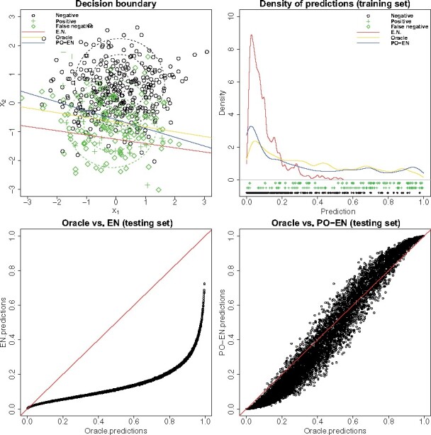
Example illustrating the advantages of the presence-only (PO-EN) model versus elastic net (EN) using a simplified simulation setting with only two covariates with correlation ρ = 0 and d = 0.8. We assume that 30% of the negative examples are in reality positive, and 10% of all examples are positives. Shown in the upper part, the decision boundary for the presence-only model is close to that of the Oracle model, an elastic net model trained with the correct labels, while the decision boundary of the naive EN model passes through the positive class. In the lower part, comparisons between predictions on the test data from the Oracle versus EN model and Oracle versus PO-EN model

3.2 Prediction accuracy of the different methods

For the training set, we randomly select n_l positive labels, and n_u background/negative labels with n_l:$n_u=1$:5 along with the corresponding DeepSEA epigenetic features. The testing set is similarly selected from the rest of the data with the same size and imbalance ratio as the training set. Results below are averages over 100 replicates. We vary the number of positive labels in the training set n_l in order to investigate the effect on the performance of the PO-EN and EN models. We focus on the four datasets with the largest number of positive labels, namely saturation mutagenesis MPRA data (in HepG2 and HEK293T), and SuRE assay data (in HepG2, K562).

We use several accuracy metrics including AUROC, AUPR and the F1 score; the F1 score is only computed for those methods that produce predicted probabilities. In terms of AUROC and AUPR, PO-EN and EN models show improved performance with increasing size of the training data as expected, and consistently outperform all other scores when the number of positive examples in the training set is at least 50 (Fig. 2). As with the simulation results (comprehensive results from simulations are in the Supplemental Material), the presence-only model performs much better than the EN in terms of the F1 score due to the fact that the EN model tends to underestimate the probabilities of regulatory effects, while the PO-EN model leads to better calibrated predicted probabilities. The DeepSEA classifiers using eQTLs or GWAS SNPs for training perform rather poorly for the MPRA datasets considered here. The functional significance score and the classifier based on HGMD variants perform better, and similar to the predicted DNase I sensitivity score (Fig. 2). Finally, FUN-LDA, CADD and Eigen generally have lower prediction accuracy relative to the PO-EN/EN models, and DeepSEA scores (DeepSEA-significance and DeepSEA-HGMD), which is expected given that these scores are either not tissues-specific (CADD and Eigen) or at a lower resolution (FUN-LDA). Note that the tissue-specific score FUN-LDA tends to perform better than the nontissue-specific scores CADD and Eigen. The PO-EN model overall performs the best in terms of all three accuracy measures.

Fig. 2.

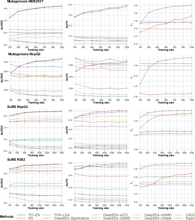
Prediction accuracy for MPRA datasets assuming different sizes for the training dataset with fixed imbalanced ratio (1:5). Average performance for three accuracy measures (AUROC, AUPR and F1 score) is shown for the different methods for each MPRA dataset (except saturation mutagenesis K562 due to small sample size)

Note that although the presence-only model avoids the issue of false negatives in the training stage, the accuracy metrics we use for evaluation in the testing stage treat the nonpositive labels as true negatives. Therefore, there is a maximum achievable accuracy (regardless of the actual metric used, e.g. AUROC, AUPR or F score) even with a perfect classifier, and therefore the accuracy values we report here need to be interpreted in this context.

3.3 Effect of class imbalance on the performance of the different methods

As we have discussed in Section 1, one of the advantages of the presence-only model is its robustness in the class imbalance setting. For the training set in here, we randomly select n_l = 100 positive labels and n_u background/negative labels with n_l:$n_u=R$, where R is the imbalance ratio. The testing set is also formed in a similar way (same size and imbalance ratio as the training set). We consider values for the imbalance ratio R from 1:2 to 1:20 depending on the dataset.

In terms of AUROC and AUPR, the PO-EN and EN models perform better than the other comparison scores (Fig. 3). Additionally, the PO-EN model performs the best in terms of the F1 score, especially as the imbalance ratio increases. Its performance decreases with increasing values of the imbalance ratio (e.g. 1:20), but less so relative to the EN model. Interestingly, for high imbalance ratio, the density of the PO-EN predictions has a mode close to 0, and additional mass distributed on the unit interval, while the EN model again underestimate the probabilities and its predictions are concentrated around the proportion of the positive labels (Fig. S2). The performance of the DeepSEA scores is as described before, with the classifier based on HGMD variants performing the best among the DeepSEA scores, but with lower accuracies than the proposed PO-EN model. As before, CADD, Eigen and FUN-LDA tends to perform worse than the PO-EN models.

Fig. 3.

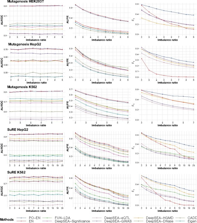
Prediction accuracy for MPRA datasets assuming different values for the imbalance ratio. Average performance for three accuracy measures (AUROC, AUPR and F1 score) is shown for the different methods for each MPRA dataset

3.4 Po-EN has better calibrated predicted probabilities relative to comparison methods

Using the MPRA experimental datasets, we also study the distributions of predicted probabilities of the different models. The predicted probabilities from the DeepSEA classifiers are shifted away from 0 and 1, and tend to concentrate around 0.5 (Fig. S2). The EN model predictions have a fairly similar distribution to those of the PO-EN model when the imbalance ratio is small or moderate. However, the density functions differ significantly when the imbalance ratio is more severe (1:7 or 1:20). In Fig. S3, we show that the PO-EN model has improved sensitivity over the EN model for different classification thresholds.

Negative correlation between MAF and PO-EN predicted probability. Based on 1 million randomly selected variants, we have observed a very small but significant negative correlation between the minor allele frequency and the predicted probability from the presence-only model: for HepG2, $r=-0.002$ (P = 0.018) and for K562, $r=-0.003$ (P = 0.002). This may suggest a slight negative selection pressure on the predicted regulatory variants. These results are concordant with those in Kircher et al. (2019) and van Arensbergen et al. (2019).

Enhancers versus promoters. We compare the predicted probabilities for variants falling in putative cis-regulatory elements, including promoters and enhancers (defined as explained in the Supplemental Material). Whereas the SuRE signals for enhancers tend to be weaker than for promoters, the predicted probabilities from the presence-only model do not seem to differ significantly between promoter and enhancer regions (Fig. S4).

3.5 Finemapping of eQTLs and GWAS variants

We show here applications to the prioritization among eQTLs for specific genes, or SNPs at GWAS loci based on the predictions of PO-EN models in relevant tissues. We focus on the comparisons here between the PO-EN model and the popular DeepSEA models, but in Supplemental Figures we also report comparisons with other functional scores including FUN-LDA, CADD and Eigen.

3.5.1 PO-EN can prioritize putative functional eQTLs in GTEx

Based on eQTL results in GTEx for two tissues related to those used here (whole blood for K562 and liver for HepG2), we have generated functional predictions using the PO-EN model on eQTLs for each eGene for the two tissues in order to identify putative functional eQTLs for these genes. The number of candidate functional eQTLs for each eGene has a median of 3, down from a median of 57 eQTLs per eGene (Fig. S5), providing a prioritized set of putative functional eQTLs for each eGene.

We next consider a specific example concerning the adjacent genes YEATS4 and LYZ with overlapping sets of eQTLs in whole blood. SuRE identified two SNPs in K562 cells, and subsequent in vitro binding proteomic experiments confirmed that variation at both SNPs may affect binding of TFs and their co-factors (van Arensbergen et al., 2019). The presence-only model predicts a high probability for these variants to be functional ($\sim 0.8$) in K562 (Fig. 4). We also compare with the predictions from DeepSEA. Regardless of which DeepSEA score we look at the predicted probabilities tend to center around 0.5. The predictions from DeepSEA-eQTL, the model trained using eQTL variants, are shown in Figure 4. As shown, this model fails to prioritize the putative functional eQTLs. However, the model trained using the HGMD labels and the functional significance score perform better and help prioritize these variants (Figs S6 and S7).

Fig. 4.

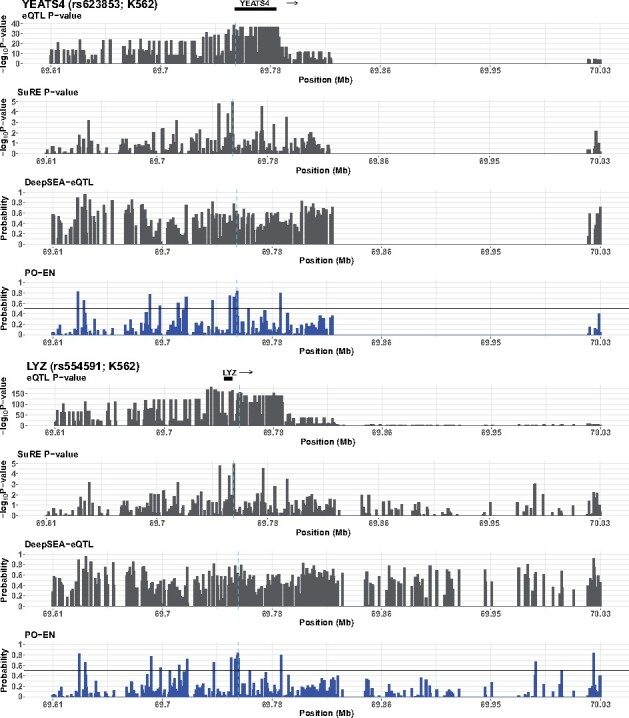
Predicted functional eQTLs in K562 for the YEATS4 and LYZ genes. In addition to PO-EN predicted probabilities, P-values from the eQTL (GTEx) and differential expression test in SuRE assay, and predicted probabilities from DeepSEA-eQTL are also shown in each region. The known functional variants are indicated with vertical broken lines

Comparing with SuRE results for eQTLs in whole blood and liver, we show that for those eQTLs with very small differential expression test P-values (e.g. $<{10}^{-14}$) in the SuRE experiment a large fraction of those (over 80%) have predicted probability greater than 0.5 in the corresponding cell line (Fig. S8). Overall, the PO-EN model leads to a higher proportion of putative regulatory variants (with predicted probability greater than 0.5) compared to the SuRE experiment, which could be due to increased sensitivity, although higher false positive rates can also play a role. Additional examples of predictions for eQTLs for several genes with good concordance between SuRE and PO-EN further illustrate this point (see Figs S9–S12).

3.5.2 PO-EN can prioritize putative functional SNPs at GWAS loci

Predictions based on pretrained PO-EN models are also useful for prioritizing putative regulatory SNPs at GWAS loci. We first focused on specific examples highlighted by van Arensbergen et al. (2019). One such example is rs4572196 residing at a GWAS locus associated with various mature red blood cell traits such as hemoglobin concentration and hematocrit, and containing $\sim 170$ genome-wide significant SNPs in high LD (Astle et al., 2016). Of these, 88 SNPs are also included on the SuRE assay. The PO-EN model leads to five SNPs having predicted probabilities greater than 0.5 in K562 in the region, with a predicted probability of $\sim 0.8$ for rs4572196 (Fig. 5). In van Arensbergen et al. (2019), they show by in vitro proteomics that several proteins exhibit differential binding activity to the two rs4572196 alleles. Another example is rs3748136 at a GWAS locus containing a total of 36 GWAS significant SNPs in high LD, associated with blood counts of reticulocytes (Astle et al., 2016). As with the first example, in van Arensbergen et al. (2019), they show by in vitro proteomics that several proteins exhibit differential binding activity to the two alleles. Of the 32 SNPs on the SuRE assay, only three have predicted probabilities greater than 0.5 in the PO-EN model, including rs3748136. A third example is a locus identified in a GWAS study for hepatitis B virus (HBV)-related hepatocellular carcinoma (HCC) (Sawai et al., 2018). This study identified 61 candidate SNPs in a ∼200 kb region. We generated predictions for HepG2 for all 48 SNPs in this region on the SuRE assay. Only three SNPs show predicted probabilities by the PO-EN model greater than 0.5, two of which, rs2735069 and rs7741418, were detected by the SuRE assay as well (Fig. 5). The predictions from the DeepSEA-GWAS model for these three loci are also shown in Figure 5, and predictions from the various DeepSEA models are reported in Figures S13–S15. Overall, the models DeepSEA-GWAS and DeepSEA-eQTL fail to prioritize the putative functional variants at these loci; the HGMD-based model and the functional significance score perform better; however, for the GWAS locus in HBV-related HCC, only the proposed PO-EN model can identify the two putative regulatory variants in HepG2.

Fig. 5.

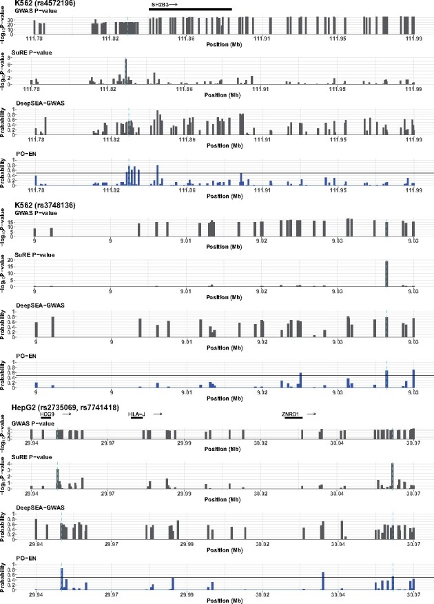
Predicted functional GWAS SNPs for three GWAS loci. In addition to PO-EN predicted probabilities, P-values from the GWAS and differential expression test in SuRE assay, and predicted probabilities from DeepSEA-GWAS are also shown in each region. The known functional variants in each region are indicated with vertical broken lines

We additionally investigated several other experimentally validated functional GWAS SNPs reported in the literature (Edwards et al., 2013). Specifically, for a set of GWAS loci with follow-up experimental evidence, we have generated predictions in HepG2 and K562 for the putative functional SNPs at these loci. We also show predictions for SNPs in 100 kb regions centered around the putative functional SNP(s). For a direct comparison with the results from the SuRE assay, we focus on those SNPs assayed on the SuRE assay (although the putative functional SNPs of interest are included regardless). Results for 11 loci with functional SNPs (Table S2) are shown in Figures 6 and S16–S24. One interesting example is the SORT1 locus on 1p13, associated with low-density lipoprotein cholesterol. The likely causal variant is rs12740374. This SNP is located in an enhancer, and it was shown that it affects its activity by creating a C/EBP TF-binding site (Musunuru et al., 2010). The predictions for this locus are shown in Figures 6 and S25. The predicted probability in HepG2 for rs12740374 is $\sim 0.9$, the highest in the region; the predicted probability in K562 is $\sim 0.77$. This particular SNP has not been assayed in the SuRE assay. This example illustrates a main advantage of the PO-EN model, namely its ability to produce predicted probabilities at any genetic variant of interest beyond those assayed in a particular experiment.

Fig. 6.

Predicted functional SNPs for SORT1 and CDKN2A loci in HepG2. In addition to PO-EN predicted probabilities, P-values from the differential expression test in SuRE assay and predicted probabilities from DeepSEA-GWAS are also shown in a 100 kb region. The known functional variants are indicated with vertical broken lines

Another interesting example is the CDKN2B-CDKN2A locus on 9p21 associated with coronary artery disease (CAD). One or two SNPs (rs10811656 or rs10757278) have been identified as putative functional at this locus; these two SNPs reside in an enhancer and disrupt a binding site for STAT1, a well-known effector of interferon signaling (Harismendy et al., 2011). We show predictions for these two SNPs in both HepG2 and K562, and for SNPs in the neighboring 100 kb region (Fig. 6). Both SNPs have higher predicted probabilities in HepG2 relative to K562, and in particular rs10811656 has a probability of 0.83 in HepG2 and 0.78 in K562. These two SNPs have been assayed on the SuRE assay, but their signal is weak and are not picked up as regulatory variants. The DeepSEA models fail to prioritize these two putative functional variants (Fig. S26). Additional results for the remaining loci in Table S2 are shown in Figures S16–S24.

3.5.3 The costimulatory locus in Alopecia Areata

We discuss here in more detail the analysis of a GWAS locus, the costimulatory locus, spanning a 270 kb region in the genome (hg19 chr2:204567170-204831755) and associated with several autoimmune disorders, including Alopecia Areata, Graves disease, type 1 diabetes, Celiac disease and rheumatoid arthritis. The costimulatory locus, one of the first loci outside the HLA region to be associated with autoimmune diseases, consists of three linkage disequilibrium (LD) blocks separated by recombination hotspots. Disease association studies consistently implicate the 129 kb LD block spanning CTLA4 and the 5ʹ end of ICOS (hg19 chr2:204687518-204816575, Fig. S27), and haplotype studies have identified two common haplotypes at this locus, along with several rare haplotypes (Brophy et al., 2006; Butty et al., 2007; Ueda et al., 2003). Studies in type 1 diabetes, Graves Disease and Celiac Disease have found increased risk of disease associated with one of the common haplotypes, and evidence for a protective effect with the other common haplotype. Here, we provide evidence of a regulatory variant that is in high LD with a coding, functional variant residing in CTLA4, both associated with Alopecia Areata, with both risk increasing alleles being on the risk increasing haplotype.

We have generated predictions in HepG2 and K562 for SNPs in a 297 kb region encompassing the costimulatory locus. For a direct comparison with the results from the SuRE assay, we focus on those SNPs assayed on the SuRE assay. As reported in Figures 7 and S28, there is one SNP, rs2352546, that is predicted regulatory in both cell lines using both the PO-EN model (predicted probability in K562 0.94 and 0.88 in HepG2) and the SuRE assay (P-value for K562 is $2 \times {10}^{-11}$ and $4.6 \times {10}^{-8}$ in HepG2). Although this SNP does not stand out in terms of its predicted probability in neither DeepSEA-GWAS nor DeepSEA-eQTL models, it is among the higher ranked SNPs for the other two models, DeepSEA-HGMD and the functional significance score. Interestingly, this regulatory SNP is located in an active enhancer in CD14+ monocytes (Fig. S29), and predicted functional in the same cell type by FUN-LDA (Backenroth et al., 2018; Fig. S30). Additionally, using predictions from the GeneHancer database, the SNP is located in an enhancer that is predicted to interact with CTLA4 based on capture Hi-C data in GM12878 and CD34+ cells (Fig. 8). rs2352546 is also tightly linked with the common functional variant rs231775 in exon 1 of CTLA4 ($R^2=0.86$), with the risk increasing allele G of rs2352546 residing on the same risk haplotype as the risk increasing G allele of the coding variant rs231775. Previous studies have shown that guanine at rs231775 is related to lower expression levels of the CTLA4 protein (Ligers et al., 2001), and demonstrate complex expression dynamics that are influenced by the cellular context and disease status (Chen et al., 2018).

Fig. 7.

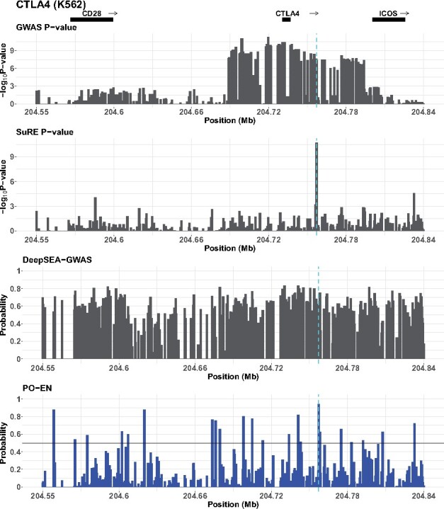
Predicted functional GWAS SNPs for the CTLA4 locus in K562. In addition to PO-EN predicted probabilities (bottom panel), P-values from the Alopecia Areata GWAS, predictions from the DeepSEA-GWAS model and P-values from the differential expression test in the SuRE assay are also shown. The putative functional variant is indicated with a vertical broken line

Fig. 8.

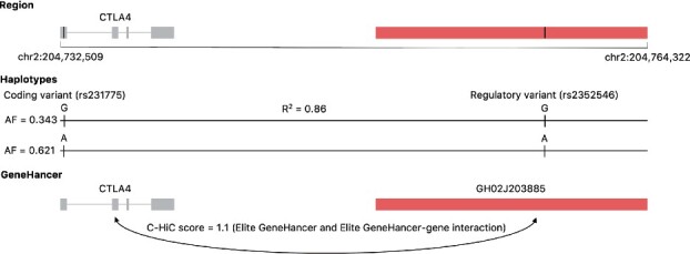
A coding variant in exligers2001ctlaon 1 of CTLA4 and a regulatory variant in an enhancer interacting with CTLA4 within the costimulatory locus. The coding and the regulatory SNPs are in tight LD, with the risk increasing alleles on the same haplotype

Using gene expression data from human scalp skin biopsies from 37 Alopecia Areata research participants collected from four National Alopecia Areata Foundation (NAAF) registry sites (see Supplemental Material for more information on the gene expression data), we have detected significant association between SNP genotypes at rs2352546 and CTLA4 expression (Fig. S31). Interestingly, this association appears nonlinear, with heterozygous AG individuals having significantly reduced expression levels, while homozygous GG individuals having higher expression levels. Such nonlinear associations could be due to interactions with other genetic variants or environmental factors, or different physiological conditions. Although our sample size is limited and results need to be validated, the increased expression for the GG genotype could potentially lead to increased penetrance of the coding variant (Castel et al., 2018). The GG genotype at the regulatory variant is almost exclusively accompanied by the GG genotype at the coding variant, and the odds ratio for the association G-G/G-G versus A-A/A-A is 1.886 [95% CI (1.474, 2.421)], while the odds ratio for the association G-G/A-A versus A-A/A-A is 1.425 [95% CI (1.193, 1.701)]. Overall, these findings suggest that the regulatory variant together with the common coding variant on the same risk haplotype may act together to increase risk to Alopecia Areata.

4 Discussion

We have proposed a semisupervised method for predicting regulatory effects at the sequence level using experimentally (MPRA) derived labels. The proposed model has the significant advantage that it can be trained based on limited experimental MPRA data in a tissue or cell type of interest to make regulatory effect predictions for single nucleotide changes genome-wide, and we show that such an approach can be substantially more accurate relative to state-of-the-art prediction models such as DeepSEA. The method is based on a presence-only model that uses data on positive responses, i.e. likely regulatory variants from MPRAs, together with a larger set of background data, and large number of functional covariates, such as epigenetic features (open chromatin, methylation, histone modifications) to build presence-only prediction models of regulatory effects in a context of interest. Our results demonstrate that the presence-only model is an effective strategy to predict regulatory effects and produces better calibrated probabilities of regulatory effects relative to existing functional prediction models. In particular, by taking into account the uncertainty in the background data, the presence-only model naturally increases the predicted probabilities of regulatory effects. The proposed model is particularly useful when trained on limited MPRA data in a cell type of interest to make predictions at previously seen or unseen variants genome-wide, and to prioritize putative regulatory variants among eQTLs or GWAS SNPs. Unlike recently proposed experimental approaches such as the SuRE assay, our presence-only model can be used to make predictions at any variant of interest, including new variants discovered in sequencing studies.

It is possible to incorporate into the presence-only model prior information on potential functional effects of variants in the genome by using an adaptive elastic net penalty. Such information is available from numerous computational prediction methods (Backenroth et al., 2018; He et al., 2018; Ionita-Laza et al., 2016; Lee et al., 2015; Zhou and Troyanskaya, 2015). Incorporating prior information from external datasets can be beneficial in this setting when the number of experimentally validated variants is limited, as it does not require to further divide the dataset for learning the weights. Additionally, given the high-dimensional nature of the problem with large number of covariates, building a penalized-likelihood model with prior weights can further reduce the dimensionality of the covariate vector, resulting in a faster computation time and better model selection.

Defining the functional consequence for a sequence change is challenging since there are many different ways a variant can have a functional effect. Many supervised methods have been proposed to predict functional effects of genetic variation, focusing on particular aspects of function, including evolutionary conservation, mutations associated with human diseases from HGMD, variants associated with complex diseases from the GWAS catalog, eQTLs, chromatin accessibility, histone modifications, etc. (Kircher et al., 2014; Lee et al., 2015; Ritchie et al., 2014; Zhou and Troyanskaya, 2015). Unsupervised methods alleviate the need to rely on labeled variants (Backenroth et al., 2018; He et al., 2018; Ionita-Laza et al., 2016), but can suffer in accuracy relative to supervised methods if high quality labels are indeed available. Here, we have proposed to use potentially regulatory variants in MPRA experiments to train prediction models since MPRAs provide more direct evidence of regulatory effects on gene expression in a context of interest. We show that, using even a small number of positive labels from an MPRA experiment, we can train classifiers with high accuracy. Given the wide applicability of MPRAs to identify regulatory variants in complex diseases, the proposed prediction model can be trained on limited MPRA data in tissues and cell types of interest (e.g. at one or several GWAS loci) to make genome-wide predictions.

The presence-only model has been implemented in an R package PO-EN and is available on the Comprehensive R Archive Network (CRAN). When MPRA data in a tissue/cell type of interest are available on limited set of variants, the package can be used to train a presence-only model to make predictions for genetic variants genome-wide.

Funding

This research has been supported by awards MH106910 and MH095797 from the National Institute of Mental Health (NIMH).

Conflict of Interest: none declared.

References

- Astle W.J. et al. (2016) The allelic landscape of human blood cell trait variation and links to common complex disease. Cell, 167, 1415–1429. [DOI] [PMC free article] [PubMed] [Google Scholar]
- Backenroth D. et al. (2018) FUN-LDA: a latent Dirichlet allocation model for predicting tissue-specific functional effects of noncoding variation: methods and applications. Am. J. Hum. Genet., 102, 920–942. [DOI] [PMC free article] [PubMed] [Google Scholar]
- Bernstein B.E. et al. (2010) The NIH roadmap epigenomics mapping consortium. Nat. Biotechnol., 28, 1045–1048. [DOI] [PMC free article] [PubMed] [Google Scholar]
- Brophy K. et al. (2006) Haplotypes in the ctla4 region are associated with coeliac disease in the Irish population. Genes Immun., 7, 19–26. [DOI] [PubMed] [Google Scholar]
- Butty V. et al. (2007) Signatures of strong population differentiation shape extended haplotypes across the human CD28, CTLA4, and ICOS costimulatory genes. Proc. Natl. Acad. Sci. USA, 104, 570–575. [DOI] [PMC free article] [PubMed] [Google Scholar]
- Castel S.E. et al. (2018) Modified penetrance of coding variants by cis-regulatory variation contributes to disease risk. Nat. Genet., 50, 1327–1334. [DOI] [PMC free article] [PubMed] [Google Scholar]
- Chawla N.V. et al. (2004) Special issue on learning from imbalanced data sets. ACM SIGKDD Explor. Newsl., 6, 1–6. [Google Scholar]
- Chen Y. et al. (2018) Ctla-4 +49 G/A, a functional T1D risk SNP, affects CTLA-4 level in Treg subsets and IA-2A positivity, but not beta-cell function. Sci. Rep., 8, 10074. [DOI] [PMC free article] [PubMed] [Google Scholar]
- Consortium E. P. et al. (2012) An integrated encyclopedia of DNA elements in the human genome. Nature, 489, 57. [DOI] [PMC free article] [PubMed] [Google Scholar]
- Edwards S.L. et al. (2013) Beyond GWASs: illuminating the dark road from association to function. Am. J. Hum. Genet., 93, 779–797. [DOI] [PMC free article] [PubMed] [Google Scholar]
- Fishilevich S. et al. (2017) Genehancer: genome-wide integration of enhancers and target genes in genecards. Database, 2017, bax028. [DOI] [PMC free article] [PubMed] [Google Scholar]
- Fithian W., Hastie T. (2014) Local case-control sampling: efficient subsampling in imbalanced data sets. Ann. Stat., 42, 1693–1724. [DOI] [PMC free article] [PubMed] [Google Scholar]
- Harismendy O. et al. (2011) 9p21 DNA variants associated with coronary artery disease impair interferon-γ signalling response. Nature, 470, 264–268. [DOI] [PMC free article] [PubMed] [Google Scholar]
- He H., Garcia E.A. (2009) Learning from imbalanced data. IEEE Trans. Knowl. Data Eng., 21, 1263–1284. [Google Scholar]
- He Z. et al. (2018) A semi-supervised approach for predicting cell-type specific functional consequences of non-coding variation using MPRAs. Nat. Commun., 9, 5199. [DOI] [PMC free article] [PubMed] [Google Scholar]
- Inoue F. et al. (2017) A systematic comparison reveals substantial differences in chromosomal versus episomal encoding of enhancer activity. Genome Res., 27, 38–52. [DOI] [PMC free article] [PubMed] [Google Scholar]
- Ionita-Laza I. et al. (2016) A spectral approach integrating functional genomic annotations for coding and noncoding variants. Nat. Genet., 48, 214–220. [DOI] [PMC free article] [PubMed] [Google Scholar]
- Karczewski K.J. et al. (2020) The mutational constraint spectrum quantified from variation in 141,456 humans. Nature, 581, 434–443. [DOI] [PMC free article] [PubMed] [Google Scholar]
- King G., Zeng L. (2001) Logistic regression in rare events data. Polit. Anal., 9, 137–163. [Google Scholar]
- Kinney J.B., McCandlish D.M. (2019) Massively parallel assays and quantitative sequence–function relationships. Annu. Rev. Genomics Hum. Genet., 20, 99–127. [DOI] [PubMed] [Google Scholar]
- Kircher M. et al. (2014) A general framework for estimating the relative pathogenicity of human genetic variants. Nat. Genet., 46, 310–315. [DOI] [PMC free article] [PubMed] [Google Scholar]
- Kircher M. et al. (2019) Saturation mutagenesis of twenty disease-associated regulatory elements at single base-pair resolution. Nat. Commun., 10, 1–15. [DOI] [PMC free article] [PubMed] [Google Scholar]
- Lee D. et al. (2015) A method to predict the impact of regulatory variants from DNA sequence. Nat. Genet., 47, 955–961. [DOI] [PMC free article] [PubMed] [Google Scholar]
- Ligers A. et al. (2001) CTLA-4 gene expression is influenced by promoter and exon 1 polymorphisms. Genes Immun., 2, 145–152. [DOI] [PubMed] [Google Scholar]
- Liu M. et al. (2018) Cost-sensitive feature selection by optimizing f-measures. IEEE Trans. Image Process., 27, 1323–1335. [DOI] [PubMed] [Google Scholar]
- Mulvey B. et al. (2020) Massively parallel reporter assays: defining functional psychiatric genetic variants across biological contexts. Biol. Psychiatry, 89, 76–89. [DOI] [PMC free article] [PubMed] [Google Scholar]
- Musunuru K. et al. (2010) From noncoding variant to phenotype via sort1 at the 1p13 cholesterol locus. Nature, 466, 714–719. [DOI] [PMC free article] [PubMed] [Google Scholar]
- Niculescu-Mizil A., Caruana R. (2005a) Obtaining calibrated probabilities from boosting. In UAI'05: Proceedings of the Twenty-First Conference on Uncertainty in Artificial Intelligence, pp. 413.
- Niculescu-Mizil A., Caruana R. (2005b) Predicting good probabilities with supervised learning. In Proceedings of the 22nd International Conference on Machine Learning, pp. 625–632.
- Phillips S.J., Elith J. (2013) On estimating probability of presence from use–availability or presence–background data. Ecology, 94, 1409–1419. [DOI] [PubMed] [Google Scholar]
- Prentice R.L., Pyke R. (1979) Logistic disease incidence models and case-control studies. Biometrika, 66, 403–411. [Google Scholar]
- Rastogi C. et al. (2018) Accurate and sensitive quantification of protein-DNA binding affinity. Proc. Natl. Acad. Sci. USA, 115, E3692–E3701. [DOI] [PMC free article] [PubMed] [Google Scholar]
- Ritchie G.R. et al. (2014) Functional annotation of noncoding sequence variants. Nat. Methods, 11, 294–296. [DOI] [PMC free article] [PubMed] [Google Scholar]
- Sawai H. et al. (2018) Genome-wide association study identified new susceptible genetic variants in HLA class I region for hepatitis B virus-related hepatocellular carcinoma. Sci. Rep., 8, 1–8. [DOI] [PMC free article] [PubMed] [Google Scholar]
- Song H., Raskutti G. (2019) Pulasso: high-dimensional variable selection with presence-only data. J. Am. Stat. Assoc., 115, 1–30. [DOI] [PMC free article] [PubMed] [Google Scholar]
- Tewhey R. et al. (2016) Direct identification of hundreds of expression-modulating variants using a multiplexed reporter assay. Cell, 165, 1519–1529. [DOI] [PMC free article] [PubMed] [Google Scholar]
- Tibshirani R. (1996) Regression shrinkage and selection via the lasso. J. R. Stat. Soc. Ser. B, 58, 267–288. [Google Scholar]
- Ueda H. et al. (2003) Association of the t-cell regulatory gene CTLA4 with susceptibility to autoimmune disease. Nature, 423, 506–511. [DOI] [PubMed] [Google Scholar]
- van Arensbergen J. et al. (2019) High-throughput identification of human SNPs affecting regulatory element activity. Nat. Genet., 51, 1160–1169. [DOI] [PMC free article] [PubMed] [Google Scholar]
- Ward G. et al. (2009) Presence-only data and the EM algorithm. Biometrics, 65, 554–563. [DOI] [PMC free article] [PubMed] [Google Scholar]
- Wasikowski M., Chen X-w. (2010) Combating the small sample class imbalance problem using feature selection. IEEE Trans. Knowl. Data Eng., 22, 1388–1400. [Google Scholar]
- Zhou J., Troyanskaya O.G. (2015) Predicting effects of noncoding variants with deep learning-based sequence model. Nat. Methods, 12, 931–934. [DOI] [PMC free article] [PubMed] [Google Scholar]
- Zou H., Zhang H.H. (2009) On the adaptive elastic-net with a diverging number of parameters. Ann. Stat., 37, 1733–1751. [DOI] [PMC free article] [PubMed] [Google Scholar]
Associated Data
This section collects any data citations, data availability statements, or supplementary materials included in this article.