Experimental and Simulation Studies on the Slug Flow in Curve Pipes

Abstract

This work focuses on the two-phase slug flow in the curve pipe, which is very common in oil/gas wells. In terms of oil and gas production, the unstable slug flow may cause several problems and reduce production. In the present work, slug flow experiments were conducted in several curve pipes for varying inflow angles and gas–liquid velocity ratios. The real-time pressure was measured at the curve pipe using the Rosemount pressure gauges, and the liquid holdup was measured using the conductivity sensors, which were used to calculate the slug length. Then, we define the dimensionless slug length φ_D = L_S/D (the ratio of slug length L to pipe diameter D), which can make the slug analysis free from the influence of different pipe diameters; φ_D is also used to analyze the change in the slug flow state. The experimental results show that the dimensionless slug length φ_D increases with the increase in the pipe curvature; φ_D first decreases and then increases with the increase in the inflow angle; φ_D also increases with the increase in the gas–liquid velocity ratio. This study adopts a dynamic slug flow model to simulate the well completion and the throttle cases under field conditions based on the hydraulic similarity principle. The pressure and liquid holdup results show that the large-scale segregated completion will lead to decreasing flow instability and the decrease in throttle opening will also lead to the decrease in flow instability.

1. Introduction

In the oil and natural gas industry, the curve section exists in horizontal wells, inclined wells, and subsea risers.^1,2 The curve section will cause the two-phase flow instability, which is the result of the change in forces on the fluid and flow direction. Several flow patterns could occur in the wells and risers; among these flow patterns, slug flow needs to be avoided. It is very unstable and could reduce the oil production,³ cause pipeline fatigue,⁴ increase corrosion,⁵ and affect the pump efficiency. With slug flow in a pipe, the liquid phase exists as liquid slugs entrained with gas bubbles, and the gas phase exists as large Taylor bubbles along the pipe. The slug flow has the characteristic of fluctuated liquid holdup and pressure.⁶⁻¹⁰ For the curve pipe case, some factors will have influences on the pressure and liquid holdups, such as the inflow angle, pipe curvature radius, and liquid–gas velocity ratio. In order to reduce the disadvantage of slug flow in a well, there are several slug control methods¹¹ that can be used during oil and gas production. Therefore, this study is mainly focused on the main factors that will influence the slug flow state in the curve section and the methods to reduce the instability of slug flow.

To study the film thickness change of annular flow in a 90° bend, Maddock et al.¹² used a range of 30–90° curve pipes that are connected after vertical pipes. They obtained the results of the circumferential variation of the film thickness. Chisholm¹³ found that the friction of two-phase flow in the elbow is inversely related to the curvature of the bend pipe and obtained an equation for predicting the two-phase pressure drop in the curve pipe.

Silva et al.¹⁴ measured the liquid holdup and length and frequency of slugs upstream and downstream of a horizontal 90° curve pipe using embedded conductive probes. They noted that the downstream slug flow characteristics of the curve pipe (velocity, frequency, liquid holdup, and length) are completely different from the upstream characteristics of the curve pipe under a fully developed slug flow state.

Using the laser technique, Ribeiro et al.¹⁵ measured the Sauter mean diameter of water droplets in a two-phase flow before and after a horizontal 90° curve pipe. They found that the diameter of water droplets increased due to the curve section and believed that this growth was the result of droplet coalescence, deposition, and entrainment at the curve pipe.

Spedding et al.¹⁶ conducted an experimental study on the factors affecting the pressure gradient of a 90° downward curve pipe. A transparent tube with a diameter of 26 mm was used. It was found that the pressure drop in the straight pipe before entering the curve pipe is much larger, which is mainly due to the throttle effect of the curve pipe. At low flow velocity, the pressure gradient at the horizontal outlet decreases, mainly because the slug flow in the vertical section becomes a stratified wavy flow after entering the horizontal section. They also found that the change in the pressure gradient is related to the total Reynolds number. The experiment facility that Omebere-Iyari and Azzopardi¹⁷ used was a connecting upstream horizontal pipeline, which had a diameter of 189 mm and a height of 52 m. They measured and proposed a time-varying liquid holdup and flow pattern of the nitrogen–oil two-phase mixture. They compared their experimental results with Taitel’s¹⁸ and found that slug flow is formed in the upstream horizontal section and propagates to the vertical pipe section under high liquid flow rates. Moreover, slug flow does not occur when the gas and liquid directly flow into the vertical pipe section.

With the further development of two-phase flow experiments, more advanced modern instruments, such as electrical capacitance tomography (ECT) and wire mesh sensor (WMS), were applied in the study of two-phase flow in inclined pipes.¹⁹ In the experimental study of Abdulkareem et al.,¹⁹ the downstream pipeline of the curve section is horizontal, while the upstream pipeline of the curve section is vertical or horizontal. The ECT probe is installed at the location of 10D upstream of the curve pipe, and the WMS is installed before the curve pipe. The probability density function (PDF) characteristics are obtained from the time-varying cross-sectional average liquid holdup; they are used to determine the flow patterns upstream and downstream of the curve pipe. They found that there are bubble flow, stratified flow, slug flow, and semiannular flow downstream of the vertical 90° pipe, while the flow pattern of the horizontal 90° curve pipe is the same as that upstream of the curve pipe.

Saidj et al.²⁰ conducted a two-phase flow experiment with a 90° upward curve pipe. As shown in Figure 1, transparent tubes with an inner diameter of 34 mm and a radius of curvature (R/D) of 5 were used. They analyzed the PDF of the liquid holdup and dimensionless slug length at different flow rates and found that from horizontal to vertical pipes, the slug frequency increases only in some of the cases; the liquid holdup downstream of the curve pipe is higher than that upstream of the curve pipe, and the slug length becomes longer after the curve section.

Figure 1.

Scheme of the slug flow in a curve pipe.

Hsu et al.²¹ conducted two-phase flow experiments in 90° upward, downward, and horizontal pipes. The inner diameters of the pipes were 5.5 and 9.5 mm, and the curvature ratio was 2R/D (5.4 and 4.2, respectively). They found that the centrifugal force and friction loss in the curve pipe with a small curvature radius are bigger than in the large curvature case, and the pressure loss of the upward curve pipe is the largest due to the appearance of vortex flow and liquid backflow. However, the curvatures of their experimental pipes are too small for the field conditions.

Bowden et al.²² measured the liquid holdup from the air–water inlet at the axial positions of 97.5D, 112.8D, and 130.8D using a WMS, including the upstream and downstream of the 90° curve pipe. The deionized water and compressed air were used as experimental media; the flow parameters of bubble flow, the influence the of 90° curve pipe, and the liquid holdup distribution were studied at a superficial liquid velocity of 3.50–5.42 m/s and a superficial gas velocity of 0.10–1.25 m/s. They measured the area-average, time-average, and volume-average liquid holdup with 27 groups of independent experiments. The distribution of time-average liquid holdup along the vertical axis and the horizontal axis is measured using the WMS. Their results showed the influence of the superficial liquid velocity and the superficial gas velocity on the gas–liquid distribution before and after the curve pipe. They also obtained the transition from the bubble flow pattern to the slug flow pattern.

Eliminating slugs with different tools and methods has been a widely concerned research topic for several years. In the early period, Yocum²³ proposed several slug control methods, which are still being adopted so far to reduce the slug.

The slug catcher is the most commonly used in the slug elimination approach. The slug catcher operates as a slug filter, and the fluctuated gas–liquid inflow will be filtered out to the stratified gas and liquid flows. McGuiness and Cooke²⁴ proposed this method in a transportation pipe to prevent unstable multiphase flow. The principle of a slug catcher in oil production is to separate the liquid and gas at the top of wells. This method is effective but has a high cost and increases the frequency of pigging operations. Thus, the biggest limitation of the slug catchers is their high cost.

Self-gas lifting is an artificial approach to make the slug cycle and the amplitude of the pressure fluctuation smaller. It creates a smaller pipeline, injecting gas from the horizontal section to the riser section, and a check valve is installed in the small pipeline to ensure one-way flow. Sarica and Tengesdal²⁵ came up with this approach in the year 2000, and it is proved that self-gas lifting could bring a smoother startup when there is a severe slugging flow. Tengesdal et al.²⁶ studied the approach of avoiding the gas compressing through separating the gas before the base section and reinjected into the curve section. The reinjected gas reduces the hydrostatic pressure, so that the slug formation will be inhibited to some extent and slug pressure fluctuations will be reduced. The disadvantage of this approach is the cost of the extra pipeline.

The choke valve method is the most studied approach in slug elimination. This is mainly due to the fact that the choking valve is an economical, convenient, and pragmatic solution.²⁹ However, there is a lack of the influence of choke valve opening on flow characteristics, and it is hard to eliminate the slug without reducing the production rate using choke valves. Storkaas and Skogestad²⁷ and Jahanshahi et al.¹ use a theoretical model to investigate the choke valve in an offshore riser well; they aimed to find the most suitable control feedback situation for two-phase flow stabilization.

Most of the slug flow studies focused on the inclined pipe; only a few slug flow research studies followed the curve pipe with interest (as shown in Figure 1). Additionally, the previous studies of two-phase flow in a curve pipe were merely concentrated on the local flow characteristics in a curve pipe and the flow parameter variations between the upstream and the downstream of the curve pipe. In the present work, slug flow experiments were conducted in several curve pipes for varying pipe curvatures, inflow angles, and gas–liquid velocity ratios. The transient pressure and liquid holdup were measured, and the dimensionless slug length φ_D was utilized to analyze the influence of pipe curvatures, inflow angles, and gas–liquid ratios on the slug flow state. Then, the dynamic curve pipe model was adopted to study different methods to reduce the flow instability in a horizontal well under field conditions based on the hydraulic similarity principle.

2. Experimental Facilities

A total of 150 groups of experiments were conducted to study the influences of different factors on the slug flow state. The main factors in the experiments are the pipe curvature, inflow angle, and gas–liquid ratio.

2.1. Experimental Setup

Air and water are used as flow media in the experiments. The flow loop consists of a horizontal pipe and a curve pipe; the outlet is connected to air, as shown in Figure 3. Measurements were taken at a temperature of 20 °C. All the pipes are made of transparent acrylic resin, which is convenient to observe and record the flow patterns. The inner diameter of the pipes is 0.05 m. The pipe curvature radius R is 1, 1.5, and 2 m; the ratio of curvature 2R/D is 20, 30, and 40; and the pipe curvature radius can be changed by replacing the curve pipe, as shown in Figure 2. There are three pressure measure points located at the entrance, the middle, and the outlet of the pipe; the liquid holdup measure point is set at the outlet of the pipe.

Figure 3.

Diagram of the gas–liquid slug flow experiment loop.

Figure 2.

Curve pipe of the experiment loop (the photos were taken by S.S.).

Gas is supplied using an air compressor and stored in a gas storage tank. The gas flow rate is controlled using a magnetic valve downstream from the gas tank and then measured using a gas mass flowmeter with the range of 0.1–100 m³/h, which has an accuracy of ±2% of the measurement range. The liquid is supplied using a centrifugal pump from a water tank and measured using a turbine flowmeter with the range of 0–1 m³/h, which has an accuracy of ±2% of the measurement range. The gas and liquid converge in a mixer; the air and water will be fully blended in the mixer and flow through the test section. Then, the pressure of the curve pipe is measured using RoseMount pressure gauges with a measurement range of 0–500 kPa, and the liquid holdup is measured using a conductivity sensor proposed by Fossa.²⁸ This method is relatively simple and can measure the liquid holdup in real time without breaking the flow pattern. It is installed at the outlet of the curve pipe, and the flow patterns and water film are recorded usingva high-speed camera. The water is then recycled into the water tank, which is connected to the test-section outlet and is open to the atmosphere.

The device uses a high-speed acquisition card to collect all the pressure and liquid holdup data and displays and stores them in the computer. The accuracy of the pressure sensor is ±0.1% of the measurement range. The measurement range of the sensor is 0–500 kpa. The accuracy of the liquid holdup sensor is ±2% of the measurement range. The liquid velocity and the gas velocity were fixed at a certain value, and the pressure and liquid holdup were measured three times. By comparing the data of pressure and liquid holdup and the number of slugs, it can be calculated that the uncertainty is within 10%, which is acceptable for the experiment.

The slug flow velocity can be obtained according to the liquid holdup data and used to analyze the slug parameters such as slug frequency and slug length. Since the distance between the two sensors of the liquid holdup device is very small, it can be considered that the geometric characteristics of the slug do not change when passing through the measuring device, as shown in Figure 5. The frequency and amplitude of liquid holdup curves obtained with the two sensors are very similar, with only a slight difference. This difference is the time that a single slug (consisting of a liquid slug entrained with small bubbles and a large bubble with a liquid film at the pipe wall) passes through two sets of sensors (as shown in Figure 4). Therefore, according to the time that the slug passes through the sensor, the velocity of the slug passing through the sensors can be calculated, which is the slug velocity at this position in the pipeline.

Figure 5.

Liquid holdup measurement unit.³⁰

Figure 4.

Liquid holdup measurement results of two groups of sensors in the same measuring unit.

Slug frequency can be calculated by the slug passing time on the two liquid holdup curves. Combined with the slug flow velocity, the slug length can be calculated in different situations.

1

All parameters and boundary conditions used in the experiments are illustrated in Table 1.

Table 1. Parameters and Boundary Conditions Used in the Experiments.

parameter	case 1	case 2	case 3	unit
pipe diameter	0.05	0.05	0.05	M
superficial gas velocity	1.0–10.0	1.0–10.0	1.0–10.0	m/s
superficial liquid velocity	0.20–0.53	0.20–0.53	0.20–0.53	m/s
temperature	20	20	20	°C
curvature	1	1.5	2	M
water density	998.3	998.3	998.3	kg/m3
gas density	1.20	1.20	1.20	kg/m3
surface tension	0.076	0.076	0.076	N/m

3. Results

3.1. Analysis of the Pipe Curvature Radius

Figure 6 shows the number of slugs that occur in the curve section during the measurement time. The measurement time is 10 s in all cases. According to the slug flow pressure characteristics under different pipe curvatures, it can be seen that with the increase in the pipe curvature radius, the slug frequency decreases from 1.1 to 1.0/s gradually, which indicates that the slug shape is relatively stable when it passes through the curve pipe with a large curvature radius, and the slug does not break into a small liquid slug and a large number of small bubbles easily. When the gas–liquid flow rate is fixed, the angular velocity of the slug ω (ω = u/R) decreases with R increasing, and it leads to the decrease in the slug frequency. Based on the analysis of experimental data, the amplitude of pressure fluctuation increases with the increase in the pipe curvature radius. The main reason is that the larger pipe curvature radius has greater hydrostatic pressure, the longer slug length, and the greater fluctuation amplitude.

Figure 6.

Number of slugs with different pipe curvatures.

In order to reflect the variation characteristics of slug length under different influence factors through experiments, the dimensionless slug length φ_D = L_S/D (the slug length L_S and pipe diameter D) is defined to make the experimental data dimensionless, so that the experimental results will not be affected by single pipe diameter and have wider applicability.

Figure 7a–c presents the probability distribution of the dimensionless slug length with different curve pipes. The dimensionless slug length distributes averagely in the range of 3.7–4.4 when the pipe curvature radius is 1 m. The dimensionless slug length distributes mainly in the range of 4.5–4.7 when the pipe curvature radius is 1.5 m. The dimensionless slug length distributes mainly in the range of 5.0–5.1 when the pipe curvature radius is 2 m. It can be concluded that with the increase in the pipe curvature radius, the distribution of L_S/D is more concentrated, which indicates that the flow is more stable.

Figure 7.

Probability distribution of the dimensionless slug length with different curvature radii: (a) curvature radius is 1 m; (b) curvature radius is 1.5 m; and (c) curvature radius is 2 m.

Comparing the curves of different pipe curvatures with different inflow angles, as shown in Figure 8, it can be found that the dimensionless L_S/D increases with the increase in the pipe curvature radius at all inflow angles. At the same time, it can be seen from the laboratory experimental data that the L_S/D curve is the largest when the inflow angle is 30°, followed by 0°; the L_S/D curves of 6 and 15° are similar. The minimum L_S/D occurred at 10°.

Figure 8.

Influence of different curvatures on the dimensionless variation L_S/D under different flow angles.

Figure 9 shows the curves of different pipe curvatures with the different gas–liquid velocity ratios. It can be found that the L_S/D increases with the increased pipe curvature under all the gas–liquid velocity ratios, which is similar to the case with different inlet angles.

Figure 9.

Influence of different curvatures on the dimensionless variation L_S/D under different gas–liquid ratios.

3.2. Analysis of the Inflow Angles

The slug frequency under different inflow angles is presented in Figure 10. When the curvature radius and gas–liquid flow rate are the same, the slug frequency decreases with the increase in the inflow angle. The main reason is that with the increase in the inclination angle, the junction between the inclined pipe and the curve pipe becomes the low section (as shown in Figure 11). Thus, the slug will block the pipeline and cause gas accumulation, resulting in the slowing down of slug generation speed, so that the slug frequency is gradually reduced as the inflow angle increases. However, the fluctuation amplitude of pressure and liquid holdup has no obvious variation when the inflow angle is changed.

Figure 10.

Number of slugs with different flow angles.

Figure 11.

Junction between the inclined pipe and the curve pipe.

In the previous section, the probability distribution of the dimensionless slug length at 0° is given, and Figure 12 shows the probability distribution characteristics of slug length under different inflow angles when the curvature radius is fixed at 1.5 m.

Figure 12.

Probability distribution of the dimensionless slug length with different inflow angles: (a) inflow angle is 0°; (b) inflow angle is 6°; (c) inflow angle is 10°; (d) inflow angle is 15°; and (e) inflow angle is 30°.

As can be seen from Figure 12a–e, with the increase in the inflow angle, the dimensionless slug length L_S/D distribution range expands from six to eight intervals, while the probability is less concentrated and the flow state is more unstable.

The variations in L_S/D with different flow angles are presented in Figure 13. With the increase in the inflow angle of the curve pipe, L_S/D decreases at first and then increases. When the inflow angle is small (the inflow angles are 0, 6, and 10°), the dimensionless slug length decreases with the increase in the inflow angle. The main reason is that when the inflow angle is relatively small, the low point of the pipe is not easy to block the gas, and the change in the inflow angle at the curve section will lead to the rupture of the slug and reduce the slug length. When the inflow angle increases to a certain extent (in the present experiment, the certain inflow angle is 15 and 30°), the L_S/D increases with the increase in the inflow angle. In this situation, it is because when the inflow angle exceeds a certain limit, the blocking effect of the low point becomes obvious, which will lead to gas accumulation and long slugs.

Figure 13.

Influence of different flow angles on the dimensionless variation L_S/D under different pipe curvatures.

The curves of different inflow angles with the different gas–liquid velocity ratios are presented in Figure 14. It can be seen that all the L_S/D curves have a low point when the inflow angle is 10°, except for the curve of a gas–liquid velocity ratio of 5.44, which is a relatively flat curve. It shows that under the slug flow conditions, no matter how the gas–liquid flow rate ratio changes, L_S/D decreases at first and then increases with the increase in the inflow angle.

Figure 14.

Influence of different flow angles on the dimensionless variation L_S/D under different gas–liquid velocity ratios.

3.3. Analysis of the Gas–Liquid Velocity Ratio

Figure 15 shows the slug frequency under different gas–liquid velocity ratios. It can be concluded that the slug frequency increases with the increase in the gas–liquid velocity ratio, and the slug frequencies are low when the gas–liquid velocity ratios are small (such as 5.44, 6.08, and 6.72). Nevertheless, the slug frequency increases obviously when the gas–liquid velocity ratio is high (such as 12.80, 14.40, and 16.00).

Figure 15.

Number of slugs with different gas–liquid velocity ratios.

Figure 16a–n presents the probability distribution of the dimensionless slug length with different gas–liquid velocity ratios. According to the distribution characteristics of L_S/D at different gas–liquid velocity ratios, it can be found that the distribution of L_S/D expands from four to eight intervals with increasing gas–liquid velocity ratio; the distribution is less concentrated when the gas–liquid velocity ratio is high, which leads to the increase in flow instability.

Figure 16.

Probability distribution of the dimensionless slug length with different gas–liquid velocity ratios: (a) gas–liquid velocity ratio is 5.44; (b) gas–liquid velocity ratio is 6.08°; (e) gas–liquid velocity ratio is 8.00; (f) gas–liquid velocity ratio is 9.60; (g) gas–liquid velocity ratio is 11.20; (h) gas–liquid velocity ratio is 12.80; (l) gas–liquid velocity ratio is 14.40; and (n) gas–liquid velocity ratio is 16.00.

As can be seen from Figure 17, the dimensionless slug length L_S/D increases with the increase in the gas–liquid velocity ratio in all pipe curvature radius situations. Under the low gas–liquid velocity ratio (gas–liquid velocity ratios are 5.44–8.00), the difference between the curve of 1 m curvature radius and the curve of 1.5 m curvature radius is very small; the slope of the 2 m-curvature radius curve is higher than that of others. Under the high gas–liquid velocity ratio (gas–liquid velocity ratios are 8.00–16.00), all the curve slopes become small, which indicates that the increase rate of L_S/D is relatively low.

Figure 17.

Influence of different pipe curvatures on the dimensionless L_S/D under different gas–liquid velocity ratios.

The L_S/D inflow angle curves under different gas–liquid velocity ratios are presented in Figure 18. It can be found that all the L_S/D curves increase with the increase in the the gas–liquid flow rate ratio. At the same time, it can be found from the laboratory experimental results that when the gas–liquid velocity ratio is low (gas–liquid velocity ratio is under 8.00), all the L_S/D curves have small differences, and the growth rate of L_S/D is faster. With the increase in the gas–liquid flow rate ratio, the curves start to have differences (gas–liquid velocity ratios are over 8.00), and the growth rate of all the curves decreases, showing that the increase rate of L_S/D gradually slows down with the increase in the gas–liquid flow rate ratio.

Figure 18.

Influence of different flow angles on the dimensionless L_S/D under different gas–liquid velocity ratios.

4. Discussions

In the previous chapter, the gas and liquid flow rate, the inflow angle, and the curvature radius are controlled in the experiments; the two-phase flow instability of each situation is analyzed by the slug probability distribution. Furthermore, simulation of flow instability and slug control of horizontal wells under field conditions is analyzed in this chapter. First of all, we consider the hydraulic similarity principle (including geometric similarity, kinematic similarity, and dynamic similarity). Motion similarity and dynamic similarity ensure that the gas–liquid velocity ratio and the inflow angles of experiments and the field situation are in the same range. Geometric similarity ensures that the curvature radius of the experiments is proportional to that of the whole well in the field situation. Therefore, the hydraulic similarity between the laboratory experiments and the wellbore under field conditions makes the simulation analysis credible.

A horizontal slug flow model had been established in a previous study,³⁰ and the influence of different factors on gas–liquid two-phase flow in horizontal wells under field conditions is analyzed by calculating the pressure and liquid holdup in horizontal wells. Besides, the methods and effects of eliminating slug flow instability in a wellbore are also discussed.

The model’s gas mass and momentum balance equations are

2

3

The model’s liquid mass and momentum balance equations are

4

5

The fluid properties and temperature of the gas and liquid phases are determined according to the standard laboratory conditions. The well diameter is selected as 0.089 m, as shown in Table 2.

Table 2. Parameters Used in the Simulations.

parameter	case 1	case 2	case 3	unit
pipe diameter	0.089	0.089	0.089	m
temperature	20	20	20	°C
curvature radius	100	250	500	m
liquid density	998.2	998.2	998.2	kg/m3
gas density	1.205	1.205	1.205	kg/m3
surface tension	0.075	0.075	0.075	N/m
liquid viscosity	1.002 × 10–3	1.002 × 10–3	1.002 × 10–3	Pa·s
gas viscosity	1.824 × 10–5	1.824 × 10–5	1.824 × 10–5	Pa·s

Based on the hydraulic principle, the horizontal well simulation results (Figures 20 and 21) show that with the increase in the well curvature radius, the fluctuation amplitude of pressure and liquid holdup decreases, and the instability also decreases. It shows that the simulation results are similar to the experimental results, which indicates the laboratory slug characteristics can be applied to the horizontal well case under field conditions.

Figure 20.

Simulated pressure of different curvatures in the field situation.

Figure 21.

Simulated liquid holdup of different curvatures in the field situation.

4.1. Influence of Well Completion on Flow Instability

This section mainly simulates the influence of different completion methods on the flow stability of horizontal wells. The curvature radius is set as 250 m, which is shown in Figure 19. Three kinds of well completion are simulated, which are the central pipe completion, small-scale segregated completion (less than 10 stages), and large-scale segregated completion (more than 20 stages). In the simulation, the whole flow in the horizontal well is divided into several flow sources to simulate the segregated completion. According to the comparison and analysis of the simulation results of the liquid holdup and pressure fluctuation of the completion models, the influence of different well completions on the flow instability is studied.

Figure 19.

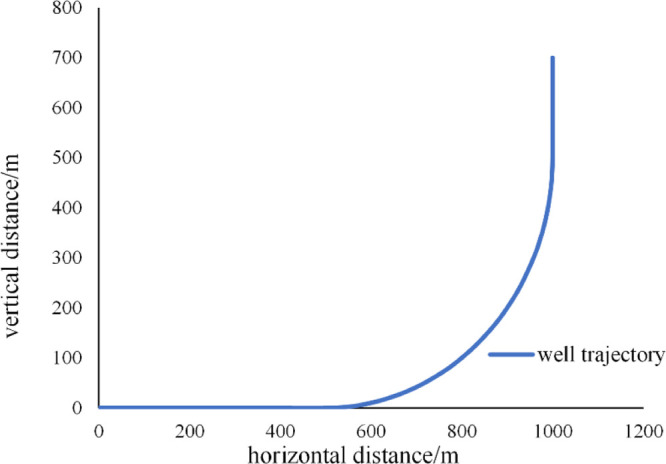
Horizontal well trajectory in the field situation.

Figure 22 shows the liquid holdup curve of three well completion cases. It can be seen that the liquid holdup fluctuation of the central pipe completion and small-scale segregated completion is relatively large, but the liquid holdup fluctuation range of large-scale segregated completion is smaller than others. The main reason is that the slug flows into the horizontal well in different locations, which leads to variable mass flow in the horizontal well. When there is small-scale segregated completion, the flow rate of each section is large, and the two-phase flow state has little change compared to a central pipe completion. In the large-scale segregated completion, the flow rate is more evenly distributed in the whole horizontal section, which makes the two-phase flow relatively stable. Therefore, the liquid holdup fluctuation is relatively small compared with that of other situations.

Figure 22.

Simulated liquid holdup curves of different well completions in the field situation.

Figure 23 shows that the overall pressure fluctuation range of the central pipe completion is large. The pressure fluctuation of small-scale segregated completion is relatively small in the first half of the simulation; then, it reduces in the second half of the simulation. The pressure fluctuation of the large-scale segregated completion in the whole simulation period is relatively small. The main reason is similar to that in the liquid holdup situation. In the case of small-scale segregated completion, the flow rate of the toe section is relatively small, while the flow rate in each completion section increases greatly, which leads to the large fluctuation of pressure.

Figure 23.

Simulated pressure curves of different well completions in the field situation.

4.2. Influence of Throttles on Flow Instability

Wellhead throttle³¹ and downhole throttle methods are analyzed in this section; the valve is set from full-open state to 10% of the full-open state. Calculation of the pressure and liquid holdup fluctuations can reflect the varied flow state.

4.2.1. Influence of the Wellhead Throttle on Flow Instability

Figures 24 and 25 present the influence of the wellhead throttle opening changes on the pressure and liquid holdup fluctuations. The opening of the wellhead throttle is fully open at 0–8000 s. It can be found that the fluctuation range of liquid holdup and pressure is relatively large, the pressure fluctuation is in the range of 4.2–4.7 MPa, and the liquid holdup fluctuation is mainly in the range of 0.10–0.90, and the flow state is very unstable. When the opening of the wellhead throttle turns down to 10% after 8000 s, it can be clearly seen that the pressure rises, but the fluctuation amplitude of the pressure and liquid holdup decreases. The pressure is in the range of 4.65–4.95 MPa, and the liquid holdup fluctuation is in the range of 0.20–0.90. With the decrease in throttle opening, the amplitude of pressure and liquid holdup fluctuation decreases, which indicates that the two-phase flow instability decreases; the increased pressure in the well will affect the oil and gas production. Therefore, the throttle opening needs to be controlled within a certain range.

Figure 24.

Simulated pressure as the wellhead throttle valve opening changes over time.

Figure 25.

Simulated liquid holdup as the wellhead throttle valve opening changes over time.

4.2.2. Influence of the Downhole Throttle on Flow Instability

Figures 26 and 27 present the influence of the downhole throttle opening changes on the pressure and liquid holdup fluctuations. The opening of the downhole throttle is fully open at 0–8000 s; it can be found that the fluctuation range of liquid holdup and pressure is relatively large, and the pressure fluctuation is in the range of 4.2–4.9 MPa, and the liquid holdup fluctuation range is mainly in the range of 0.10–0.90, and the flow state is very unstable. When the opening of the downhole throttle turns down to 10% after 8000 s, it can be clearly seen that the pressure rises, and the fluctuation amplitude of the pressure and liquid holdup decreases. The pressure is in the range of 4.7–5.3 MPa, and the liquid holdup fluctuation is in the range of 0.15–0.90. The liquid holdup and pressure trend like the wellhead throttle’s case, meaning that with the decrease in throttle opening, the amplitude of pressure and liquid holdup fluctuation decreases, but the amplitude decrease is less than in the wellhead throttle’s case.

Figure 26.

Simulated pressure curve as the downhole throttle valve opening changes over time.

Figure 27.

Simulated liquid holdup curve as the downhole throttle valve opening changes over time.

Based on the simulation study, it is found that for the wellhead throttle and downhole throttle situations, the pressure in the wellbore will increase due to the turning down of throttle opening, which also will lead to the reduction in oil production. Therefore, when the throttle method is used to restrain the slug flow instability, it is suggested that the opening of the throttle should not be less than 10%. Under these conditions, severe slug flow can be restrained to a certain extent, and the upstream pipeline pressure is not too high.

5. Conclusions

This study constructed the experimental facility of gas–liquid two-phase flow in curve pipes and carried out slug flow experiments with different curvature radii, inflow angles, and gas–liquid flow velocity ratios. Based on the defined dimensionless slug length φ_D = L_S/D, the experimental results will not be affected by the pipe diameter, and the results will be more adaptable. The L_S/D distributions and variation were calculated to illustrate the influences of different factors on the slug flow characteristics. With the increase in the curvature radius, the instability of the slug flow decreases. With the increase in the inflow angle, the instability of the slug flow increases. With the increase in the gas–liquid velocity ratio, the instability of the slug flow increases.

Based on the hydraulic similarity principle, this work simulated the influences of different well completions and well throttle methods on the two-phase flow instability. The two-phase flow state of large-scale segregated completion is more stable than in the cases of central pipe completion and small-scale segregated completion. The turning down of the throttle opening restrained the slug flow instability but will lead to the increase in pressure in the well.

This study can provide a guide for predicting the slug flow state in the curve section, which is important to the improvement of flow stability.

Glossary

Nomenclature

p

pressure

x

horizontal axial coordinate

y

vertical axial coordinate

A

area

L

slug length

v

slug velocity

f

slug frequency

S

wetted perimeter and interfacial width

F_D

drag force of bubbles in the liquid slug

u

velocity

g

gravitational acceleration

h

height of the liquid level

t

time

c

sound velocity in gas

D

hydraulic diameter

Glossary

Greek Letters

α

void fraction

β

liquid level angle

ρ

density

θ

angle corresponding to the arc length of the pipe

μ

viscosity

Glossary

Subscripts

l

liquid phase

g

gas phase

i

interface

The authors declare no competing financial interest.

Notes

The data used to support the findings of this study are available from the corresponding author upon request.

References

- Jahanshahi E.; Skogestad S.; Helgesen A. H. Controllability analysis of severe slugging in well-pipeline-riser systems. IFAC Proc. Vol. 2012, 45, 101–108. 10.3182/20120531-2-no-4020.00014. [DOI] [Google Scholar]
- De Henau V.; Raithby G. D. A study of terrain-induced slugging in two-phase flow pipelines. Int. J. Multiphase Flow 1995, 21, 365–379. 10.1016/0301-9322(94)00081-t. [DOI] [Google Scholar]
- Isaac O. A.; Cao Y.; Lao L.; Yeung H.. Production potential of severe slugging control systems. In 18th IFAC World Congress, 2011, pp 10869–10874.
- Hill T. J.; Wood D. G.. Slug Flow: Occurrence, Consequences, and Prediction; University of Tulsa Centennial Petroleum Engineering Symposium, 1994. [Google Scholar]
- Kang C.; Wilkens R.; Jepson W. P.. The effect of slug frequency on corrosion in high pressure, inclined pipelines. NACE International. Paper no. 20, 1996.
- Orkiszewski J. Predicting two-phase pressure drops in vertical pipe. J. Pet. Technol. 1967, 19, 829–838. 10.2118/1546-pa. [DOI] [Google Scholar]
- Beggs D. H.; Brill J. P. A study of two-phase flow in inclined pipes. J. Pet. Technol. 1973, 25, 607–617. 10.2118/4007-pa. [DOI] [Google Scholar]
- Dukler A. E.; Wicks M.; Cleveland R. G. Frictional pressure drop in two-phase flow: B. An approach through similarity analysis. AIChE J. 1964, 10, 44–51. 10.1002/aic.690100118. [DOI] [Google Scholar]
- Aziz K.; Govier G. W. Pressure drop in wells producing oil and gas. J. Can. Pet. Technol. 1972, 11, 38–48. 10.2118/72-03-04. [DOI] [Google Scholar]
- Grolman E.; Fortuin J. M. H. Gas-liquid flow in slightly inclined pipes. Chem. Eng. Sci. 1997, 52, 4461–4471. 10.1016/s0009-2509(97)00291-1. [DOI] [Google Scholar]
- Lahey R. T., Jr.Boiling Heat Transfer: Modern Developments and Advances; Elsevier Science, 2013. [Google Scholar]
- Maddock C.; Lacey P. M. C.; Patrick M. A. The structure of two-phase flow in a curved pipe. Inst. Chem. Eng. Symp. Ser. 1974, 38, 1–22. [Google Scholar]
- Chisholm D. Two-phase flow in bends. Int. J. Multiphase Flow 1980, 6, 363–367. 10.1016/0301-9322(80)90028-2. [DOI] [Google Scholar]
- Silva F. S.; Gómez A. H.; Velázquez M. T.. Experimental characterization of air water slug flow through a 90° horizontal elbow. Two Phase Flow Modeling and Experimentation; Edizioni ETS, 1999, pp 827–834. [Google Scholar]
- Ribeiro A. M.; Bott T. R.; Jepson D. M. The influence of a bend on drop sizes in horizontal annular two-phase flow. Int. J. Multiphase Flow 2001, 27, 721–728. 10.1016/s0301-9322(00)00038-0. [DOI] [Google Scholar]
- Spedding P. L.; Benard E. Gas–liquid two phase flow through a vertical 90° elbow bend. Exp. Therm. Fluid Sci. 2007, 31, 761–769. 10.1016/j.expthermflusci.2006.08.003. [DOI] [Google Scholar]
- Omebere-Iyari N. K.; Azzopardi B. J.. Gas/liquid flow in a large riser: effect of upstream configuration. 13th International Conference on Multiphase Production Technology; BHR Group, 2007.
- Taitel Y.; Barnea D.; Dukler A. E. Modelling flow pattern transitions for steady upward gas-liquid flow in vertical tubes. AIChE J. 1980, 26, 345–354. 10.1002/aic.690260304. [DOI] [Google Scholar]
- Abdulkareem L. A.Tomographic Investigation of Gas–Oil Flow in Inclined Risers; University of Nottingham, 2011. [Google Scholar]
- Saidj F.; Kibboua R.; Azzi A.; Ababou N.; Azzopardi B. J. Experimental investigation of air–water two-phase flow through vertical 90° bend. Exp. Therm. Fluid Sci. 2014, 57, 226–234. 10.1016/j.expthermflusci.2014.04.020. [DOI] [Google Scholar]
- Hsu L.-C.; Chen I. Y.; Chyu C.-M.; Wang C.-C. Two-phase pressure drops and flow pattern observations in 90 bends subject to upward, downward and horizontal arrangements. Exp. Therm. Fluid Sci. 2015, 68, 484–492. 10.1016/j.expthermflusci.2015.06.012. [DOI] [Google Scholar]
- Bowden R. C.; Lessard É.; Yang S.-K. Void fraction measurements of bubbly flow in a horizontal 90° bend using wire mesh sensors. Int. J. Multiphase Flow 2018, 99, 30–47. 10.1016/j.ijmultiphaseflow.2017.09.009. [DOI] [Google Scholar]
- Yocum B. T.Offshore riser slug flow avoidance: mathematical models for design and optimization. In SPE European Meeting; OnePetro, 1973, April.
- McGuinness M.; Cooke D.. Partial stabilisation at st. Joseph. In The Third International Offshore and Polar Engineering Conference; International Society of Offshore and Polar Engineers, 1993, January.
- Sarica C.; Tengesdal J. Ø.. A new technique to eliminate severe slugging in pipeline/riser systems. In SPE annual technical conference and exhibition; Society of Petroleum Engineers, 2000, January.
- Tengesdal J. Ø.; Sarica C.; Thompson L.. Severe slugging attenuation for deepwater multiphase pipeline and riser systems. In SPE Annual Technical Conference and Exhibition; Society of Petroleum Engineers, 2002, January.
- Storkaas E.; Skogestad S. Controllability analysis of two-phase pipeline-riser systems at riser slugging conditions. Contr. Eng. Pract. 2007, 15, 567–581. 10.1016/j.conengprac.2006.10.007. [DOI] [Google Scholar]
- Fossa M. Design and performance of a conductance probe for measuring the liquid fraction in two-phase gas-liquid flows. Flow Meas. Instrum. 1998, 9, 103–109. 10.1016/s0955-5986(98)00011-9. [DOI] [Google Scholar]
- Zheng G.; Brill J. P.; Taitel Y. Slug flow behavior in a hilly terrain pipeline. Int. J. Multiphase Flow 1994, 20, 63–79. 10.1016/0301-9322(94)90006-x. [DOI] [Google Scholar]
- Shi S.; Wu X.; Han G.; Zhong Z.; Li Z.; Sun K. Numerical Slug Flow Model of Curved Pipes with Experimental Validation. ACS Omega 2019, 4, 14831–14840. 10.1021/acsomega.9b01426. [DOI] [PMC free article] [PubMed] [Google Scholar]
- Xing L.; Yeung H.; Shen J.; Cao Y. A new flow conditioner for mitigating severe slugging in pipeline/riser system. Int. J. Multiphase Flow 2013, 51, 65–72. 10.1016/j.ijmultiphaseflow.2012.12.004. [DOI] [Google Scholar]