The importance of having a conceptual stage when reporting non-randomized studies

Abstract

Formal guidelines for statistical reporting of non-randomized studies are important for journals that publish results of such studies. Although it is gratifying to see some journals providing guidelines for statistical reporting, we feel that the current guidelines that we have seen are not entirely adequate when the study is used to draw causal conclusions. We therefore offer some comments on ways to improve these studies. In particular, we discuss and illustrate what we regard as the need for an essential initial stage of any such statistical analysis, the conceptual stage, which formally describes the embedding of a non-randomized study within a hypothetical randomized experiment.

1. Introduction

According to Cochran (1965):

Dorn (1953) recommended that the planner of an observational study should always ask himself¹ the question, “How would the study be conducted if it were possible to do it by controlled experimentation?”.

By proposing to begin by conceptualizing a related controlled experiment, Dorn’s advice set the stage for the estimation of the causal effect of an exposure, whether randomized or not.

Recently, there has been relatively extensive discussions about how to report empirical evidence from non-randomized studies in applied fields such as medicine, epidemiology, and social science. Even though we agree with many aspects of these published guidelines², we think that (i) some of their points should be stated more forcefully and (ii) some important points have been omitted. More specifically, we feel that the guidelines that we have seen are inadequate in at least one important aspect: A non-randomized study that estimates causal effects using Fisherian p-values or other common measures of uncertainty, such as Neymanian confidence intervals for estimands, should always be explicitly embedded within hypothetical randomized experiments; without this step, any probabilistic statements generally have little formal Fisherian or Neymanian foundation. Moreover, the results from a particular proposed hypothetical randomized experiment should be challenged by plausible deviations from the assumed randomized assignment mechanism using sensitivity analyses, which influence the discussion of results. Our recommendations apply to any non-randomized study estimating the effects of causal (i.e., manipulable) factors.

More explicitly, we present a sequence of, what we regard as essential steps (i.e., conceptual, design, statistical analysis, sensitivity analysis, and summary stages) that we believe need to be undertaken before summarizing empirical evidence of a non-randomized study (Figure 1); here, we expand especially on the conceptual stage because it is critical yet often omitted. Note that the standard statistical approach, which immediately plunges into the statistical analysis stage (i.e., regressing the observed outcome on the observed treatment and background variables), effectively proceeds as if the study were randomized with the statistical analyses reported as if the authors were following a pre-specified statistical analysis plan (SAP).

Figure 1:

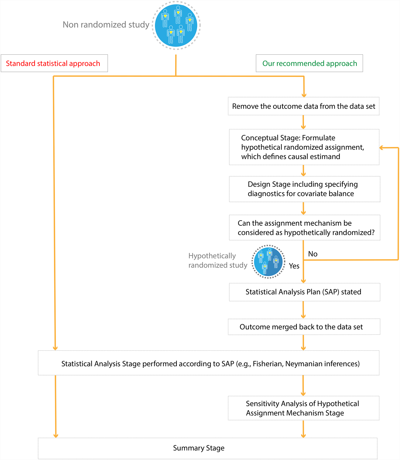
Contrasting two approaches to the analysis of non-randomized studies of causal effects.

Moreover, one of the negative aspects of the recent focus on machine learning contributions to causal inference is the subsequent focus on mechanical details for creating balance in background covariates (i.e., design stage), without any real concern for the conceptual stage, e.g., Tarr and Imai (2021).

2. The need of a conceptual stage when reporting the statistical analysis of a non-randomized study that estimates causal effects

A prespecified SAP is required for essentially all clinical trials to be approved by the US Food and Drug Administration (US Department of Health and Human Services, Food and Drug Administration et al., 1998). This systematic requirement and its public availability together force the validity and transparency of the resultant studies, and enhance the chance for the production of reproducible results. For a specific example of the possible consequences when this step is omitted, consider a recent controversial non-randomized clinical study examining the effect of hydroxychloroquine treatment on COVID-19 (Gautret et al., 2020). This study was approved by the French National Agency for Drug Safety and the French Ethic Committee, and although we could find some published information on the primary and secondary endpoints and their evaluation timepoints, we could not find any prespecified SAP on the EU Clinical Trial Register (Number 2020-000890-25). Consequently, we have little way to access whether the results in the publication should be regarded as simply exploratory.

Although some journals (e.g., NEJM, JAMA) wisely emphasize the need for a prespecified SAP, not only for randomized trials but also for non-randomized studies, we feel that this feature should be considered essential for all applied studies to ensure constructive debates of their results and conclusions. We too have previously advocated this critically important point, but even more extensively and forcefully including the explicit embedding aspect (Rubin, D. B., 2007; Rubin, D. B., 2008; Bind, M. A. and Rubin, 2017), as have others before us (Freedman, 2005; 2006). In particular, applied journals should demand that the SAP of any non-randomized study that estimates causal effects using standard frequentist statistics include the specification of an assumed hypothetical randomized experiment that generates the basis for Fisherian p-values or Neymanian confidence intervals.

Of course, the study of an intervention is not the topic of all scientific questions: most simply, there are two types of variables describing exposures, the modifiable ones, also called (treatment) factors, and the non-modifiable ones, also called blocks or strata. Causal relationships focus on treatment factors, whereas blocks allow us to understand differing susceptibility of different kinds of units to various treatments by examining how treatment effects vary across strata of units.

The causal inference framework illustrated in Figure 1 has been successfully implemented in recent observational studies examining whether air pollution exposure triggers multiple sclerosis relapses (Sommer et al., 2021a) or changes in human gut microbiome (Sommer et al., 2021b). We now provide some additional examples.

Example 1:

There is no need for the above conceptual stage for studies descriptively examining the role of non-modifiable variables, for instance, sex. Observing outcome differences between blocks (e.g., observing that males compared to females from the same population have greater risks of dying from COVID-19) is a descriptive statement, as opposed to a causal one. We believe the term “causal effect” is ideally reserved to describe the result of a possible intervention versus the absence of that intervention, i.e., the involvement of a (modifiable) factor at two or more levels, which can be studied within blocks. In this context, non-randomized studies with both modifiable and non-modifiable variables should be embedded within hypothetical randomized block experiments.

Example 2:

Consider studies that focus on the effects of meteorological or natural conditions, such as heat waves, rainfall (Sommer et al., 2018), earthquake (Zubizarreta et al., 2013), on an outcome (e.g., daily number of crimes, deaths in a city, depression). To formulate the causal question in terms of a hypothetical randomizable intervention, we have to posit that “Mother Nature” randomizes the occurrence of heat waves (or rainfall, or earthquake) given background covariates defining blocks, which usually we do not find entirely satisfactory, especially because such formulations do not envision any concrete policy intervention that would encourage or discourage the natural event. However, the effect of public “cooling centers”, implemented during the summer 2020 in Boston during a heat alert, could be an interesting question to investigate, e.g., hypothetically by randomly assigning the locations to have or not have some centers, within the city. We have only seen such a concrete proposal being actually investigated, in a few contexts, e.g., a needle exchange program, Frangakis et al. (2004).

Example 3:

Suppose we wish to estimate the causal effect of the creation of “bicycle lanes on streets” on air pollution concentrations. The goal would be to formulate the causal question using potential outcomes described in terms of hypothetical randomized bicycle-lane-related interventions. For instance, suppose that, each year, city mayors decide, at random within levels of covariates (e.g., region, city size, average socio-economic status), to create new bicycle lanes within their cities to examine whether annual air pollution concentrations would decrease with more bicycle lanes. Such urban bicycle-friendly policies have been differentially implemented across cities worldwide, e.g., Rojas-Rueda et al. (2011; 2012; 2013). Table 1 reveals the arguable plausibility of this hypothetical intervention.

Table 1:

Top twenty most bicycle-friendly cities in the world from 2013 to 2019 (Copenhagenize Design Company).

Ranking	2013	2015	2017	2019
1	Amsterdam	Copenhagen	Copenhagen	Copenhagen
2	Copenhagen	Amsterdam	Utrecht	Amsterdam
3	Utrecht	Utrecht	Amsterdam	Utrecht
4	Seville	Eindhoven	Strasbourg	Antwerp
5	Bordeaux	Malmoe	Malmoe	Strasbourg
6	Nantes	Nantes	Bordeaux	Bordeaux
7	Antwerp	Bordeaux	Antwerp	Oslo
8	Eindhoven	Strasbourg	Ljubljana	Paris
9	Malmoe	Antwerp	Tokyo	Vienna
10	Berlin	Seville	Berlin	Helsinki
11	Dublin	Barcelona	Barcelona	Bremen
12	Tokyo	Ljubljana	Vienna	Bogota
13	Munich	Dublin	Paris	Barcelona
14	Montreal	Buenos Aires	Seville	Ljubljana
15	Nagoya	Berlin	Munich	Berlin
16	Rio de Janeiro	Minneapolis	Nantes	Tokyo
17	Barcelona	Paris	Hamburg	Taipei
18	Budapest	Hamburg	Helsinki	Montreal
19	Paris	Munich	Oslo	Vancouver
20	Hamburg	Montreal	Montreal	Hamburg

We denote the bicycle-related intervention by W_i, which equals 1 if it is implemented by January 1^st 2019 in a city i, and 0 otherwise. First, assume that all interventions were equally randomized given background covariates, denoted X, which are pre-2019 city characteristics, e.g., P(W_i = 1 | X) =0.5. Let Y_i(W_i = 1) and Y_i(W_i = 0) be the potential outcomes (e.g., 2019-averaged PM_2.5 concentrations) had the city created bicycle lanes as of January 1^st 2019 or not. To assess the effect of this hypothetical intervention on air pollution concentrations, the goal is to estimate the following causal estimand under the Stable Unit Treatment Value Assumption (Rubin, 1980):

$$\tau ≔\frac{1}{N}\sum _{i=1}^N\left(Y_i\left(W_i=1\right)-Y_i\left(W_i=0\right)\right).$$

Of course, the randomness of each mayor’s decision seems implausible. We could instead propose using a randomized encouragement design (Holland, 1988; Rubin, D. B., 2011; Zell et al., 2013) as the template and assume that mayors are randomly encouraged or not to create new bicycle lanes in their city (Z_i). This template seems more plausible to us than an experiment where mayors are forced to comply with the assigned randomization, as we now describe.

The encouragement effect on the bicycle line creation (e.g., Z_i on W_i) is a causal question that can be of practical interest for urban planners and policy makers. However, without extraneous assumptions, the “intention-to-treat” (ITT) causal question, where urban planners are forced to comply with their assignment, provides only indirect insights about the effectiveness of the encouragement intervention itself on the outcome. Therefore, in this finite population of mayors, the embedding should be extended to consider a hypothetical randomized experiment with two-sided non-compliance. Let W_i(Z_i=0) and W_i(Z_i=1) be the potential outcome for creation of bicycle lanes that would be implemented by January 1^st 2019 had the mayor of city i been encouraged to do so or not. Then, we are interested in estimating the “intention-to-treat” effect, not among all cities, but rather in the compliers indicated by “co”, which are units defined by their potential outcomes W_i(Z_i = 1) = 1 and W_i(Z_i = 0) = 0, because under the common monotonicity assumption (i.e., no defier, Angrist et al. (1996)), this set of cities is the only set of cities that can be observed with and without bicycle lanes:

$${\tau }_{co}=\frac{1}{N_{co}}\sum _{i\in co}\left(Y_i\left(Z_i=1,W_i\left(Z_i=1\right)=1\right)-Y_i\left(Z_i=0,W_i\left(Z_i=0\right)=0\right)\right).$$

Finally, suppose the ultimate goal is to estimate the causal effect of air pollution on cardiovascular disease. A non-randomized study could examine the effect of the creation of bicycle lanes that will proxy for encouraging the reduction of vehicle traffic (Z_i), and thereby decreasing air pollution concentrations (W_i). In this case, the embedding would again involve the formulation of a hypothetical randomized experiment with two-sided non-compliance.

Recent studies have actually capitalized on meteorological “instrumental variables” (i.e., indicator variables for which the “unconfoundedness” assumption (Rubin, 1990) is assumed to hold), such as height of the planetary boundary layer, wind speed, and air pressure, to estimate the effect of air pollution on health outcomes, e.g., Schwartz et al. (2018); here, the description of a hypothetical intervention modifying such meteorological factors would involve “Mother Nature”.

Example 4:

Suppose we are interested in estimating the role that air pollution plays in COVID-19. There are different ways to formulate this imprecise question. We could focus on the conditional causal effects of ambient air pollution (W_i=1 for high and W_i=0 for low concentrations) on mortality among the blocks of units diagnosed to have COVID-19 or not, B_i=B⁺ if unit i is COVID-19 positive, B_i=B⁻ otherwise, and consider a hypothetical randomized block experiment for the embedding, where pollution is the randomized treatment factor, where τ(B⁺) and τ(B⁻) are the average causal effects among the B⁺ and B⁻ blocks.

Or, we could examine whether air pollution and COVID-19 are interacting (causal) factors for death. Interestingly, similar causal questions have been addressed in randomized in vitro studies (Groulx et al., 2018; Wang et al., 2018). However, randomizing humans to coronavirus (SARS-CoV-2) infections is unethical. So instead, we could “mimic” a two-factor randomized experiment and examine whether air pollution (W_i,1) and SARS-CoV-2 vaccination (W_i,2) are interacting causal factors for death (Y_i). Conducting a randomized clinical trial would be the “gold standard” to estimate this interaction. But, a more common epidemiological approach when the outcome is rare is to conduct a “case-control” study. We prefer calling such a study, a “case-noncase” study, to reserve the term “control” for the baseline level of treatment factor. A standard statistical approach simply regresses logit P(Y_i=1) on a possibly complicated function of air pollution, SARS-CoV-2 vaccination, and background covariates (X_i). We view this strategy as inappropriate, at least without elaboration. Instead, we prefer considering the target study population, from which the cases and non-cases arose, for which we want to draw causal inferences (Andric, 2015).

More specifically, to do so, we would proceed in four major steps conducted by two distinct and isolated analysts, or teams:

1. [Analyst 1] With access to all observed data, multiply-impute all missing potential outcomes (i.e., Y_i: death) under both treatments (i.e., W_i,1: high air pollution and W_i,2: SARS-CoV-2 vaccination) given covariates in the target population. This will also involve multiply-imputing X values for the unsampled units (i.e., indexed by N_cn+1 to N in Table 2).

2. [Analyst 1] Strip the outcome data from this multiply-imputed non-randomized data sets and provide them to other analyst.

3. [Analyst 2] Embed the resulting multiply-imputed data sets into a hypothetical two-factor (i.e., W_i,1: high vs. low air pollution and W_i,2: SARS-CoV-2 vaccination vs. not) randomized experiment, including a SAP.

4. [Analyst 2] Analyze the resulting data from the hypothetical experiment following the a priori defined SAP formulated in Step 3. Causal estimands of interest are the main effect of high vs. low air pollution, the main effect of SARS-CoV-2 vaccination vs. not, and their interaction. Respectively, these are defined by:

   • ${\tau }_{W_1}≔\frac{1}{2N}{\sum }_{i=1}^N\left(Y_i\left(W_{i,1}=1,W_{i,2}=0\right)-Y_i\left(W_{i,1}=0,W_{i,2}=0\right)+Y_i\left(W_{i,1}=1,W_{i,2}=1\right)-Y_i\left(W_{i,1}=0,W_{i,2}=1\right)\right)$
   • ${\tau }_{W_2}≔\frac{1}{2N}{\sum }_{i=1}^N\left(Y_i\left(W_{i,1}=0,W_{i,2}=1\right)-Y_i\left(W_{i,1}=0,W_{i,2}=0\right)+Y_i\left(W_{i,1}=1,W_{i,2}=1\right)-Y_i\left(W_{i,1}=1,W_{i,2}=0\right)\right)$
   • ${\tau }_{W_1*W_2}≔\frac{1}{2N}{\sum }_{i=1}^N\left(\left(Y_i\left(W_{i,1}=1,W_{i,2}=1\right)-Y_i\left(W_{i,1}=0,W_{i,2}=1\right)\right)-\left(Y_i\left(W_{i,1}=1,W_{i,2}=0\right)-Y_i\left(W_{i,1}=0,W_{i,2}=0\right)\right)\right)$

Table 2:

Observed and missing data table (Case-noncase study, units indexed by 1 to N_cn, Target population study: units indexed by 1 to N)

Unit i	Wi,1	Wi,2	Xi	Yi(Wi,1=0, Wi,2=0)	Yi(Wi,1=0, Wi,2=1)	Yi(Wi,1=1, Wi,2=0)	Yi(Wi,1=1, Wi,2=1)
1	0	1	X1	?	$Y_1^{obs}$	?	?
…	…	…	…	…	…	…	…
Ncn	1	1	$X_{N_{cn}}$	?	?	?	$Y_{N_{cn}}^{obs}$
Ncn+1	?	?	?	?	?	?	?
…	?	?	?	?	?	?	?
…	?	?	?	?	?	?	?
N	?	?	?	?	?	?	?

3. Conclusions

We strongly believe that embedding non-randomized studies in hypothetical randomized experiments, as implied by Dorn’s advice conveyed by Cochran, is an essential step to obtain transparent, though hypothetical, randomization-based p-values or confidence intervals. We believe that a non-randomized study lacking such a conceptual stage cannot generate statistical statements that have any real scientific meaning, even hypothetical; we must remember that a randomized assignment mechanism, actual or posited, is required for valid Fisherian or Neymanian inferences. And these inferences change as the specification of the assignment mechanism changes, as illustrated in Bind and Rubin (2017; 2020). When reporting the statistical analysis of a hypothetical randomized study, the results based on a particular, but hypothetically, assignment generally should be accompanied with a sensitivity analysis, e.g., Rosenbaum (2010), Bind and Rubin (2020), exposing how answers might change as assumptions about the hypothetical assignment mechanism change.

References

- 1.Andric N, & Harvard University. Graduate School of Arts Sciences. (2015). Exploring Objective Causal Inference in Case-Noncase Studies under the Rubin Causal Model.
- 2.Angrist JD, Imbens GW, and Rubin DB (1996) Identification of causal effects using instrumental variables” (with discussion). Journal of the American Statistical Association 91:444–472. [Google Scholar]
- 3.Bind MA, Rubin DB (2020) When possible, report a fisher-exact p-value and display its underlying null randomization distribution. Proceedings of the National Academy of Sciences of the United States of America. [DOI] [PMC free article] [PubMed] [Google Scholar]
- 4.Bind MA, Rubin DB (2017) Bridging observational studies and randomized experiments by embedding the former in the latter. Stat Methods Med Res (England) 962280217740609. [DOI] [PMC free article] [PubMed] [Google Scholar]
- 5.Cochran WG (1965) The planning of observational studies of human populations (with discussion). Journal of the Royal Statistical Society. Series A.General (London) 128:234. [Google Scholar]
- 6.Frangakis CE, Brookmeyer RS, Varadhan R, Safaeian M, Vlahov D, Strathdee SA (2004) Methodology for evaluating a partially controlled longitudinal treatment using principal stratification, with application to a needle exchange program. J Am Stat Assoc (United States) 99:239–249. [DOI] [PMC free article] [PubMed] [Google Scholar]
- 7.Freedman DA (2006) Statistical models for causation: What inferential leverage do they provide? Eval Rev (Thousand Oaks, CA) 30:691–713. [DOI] [PubMed] [Google Scholar]
- 8.Freedman DA (2005) Linear statistical models for causation: A critical review. Encyclopedia of Statistics in Behavioral Science. [Google Scholar]
- 9.Gautret P, Lagier JC, Parola P, Hoang VT, Meddeb L, Mailhe M, Doudier B, Courjon J, Giordanengo V, Vieira VE, Dupont HT, Honore S, Colson P, Chabriere E, La Scola B, Rolain JM, Brouqui P, Raoult D (2020) Hydroxychloroquine and azithromycin as a treatment of COVID-19: Results of an open-label non-randomized clinical trial. Int J Antimicrob Agents (Netherlands) 105949. [DOI] [PMC free article] [PubMed] [Google Scholar] [Retracted]
- 10.Groulx N, Urch B, Duchaine C, Mubareka S, Scott JA (2018) The pollution particulate concentrator (PoPCon): A platform to investigate the effects of particulate air pollutants on viral infectivity. Science of the Total Environment 628–629:1101–1107. [DOI] [PubMed] [Google Scholar]
- 11.Harrington D, D’Agostino RB S, Gatsonis C, Hogan JW, Hunter DJ, Normand ST, Drazen JM, Hamel MB (2019) New guidelines for statistical reporting in the journal. N Engl J Med (United States) 381:285–286. [DOI] [PubMed] [Google Scholar]
- 12.Holland PW (1988) Causal inference, path analysis, and recursive structural equations models. Sociological Methodology 18:449–484. [Google Scholar]
- 13.Rojas-Rueda D, de Nazelle A, Teixido O, Nieuwenhuijsen MJ (2013) Health impact assessment of increasing public transport and cycling use in barcelona: A morbidity and burden of disease approach. Prev Med (United States) 57:573–579. [DOI] [PubMed] [Google Scholar]
- 14.Rojas-Rueda D, de Nazelle A, Teixido O, Nieuwenhuijsen MJ (2012) Replacing car trips by increasing bike and public transport in the greater barcelona metropolitan area: A health impact assessment study. Environ Int (Netherlands) 49:100–109. [DOI] [PubMed] [Google Scholar]
- 15.Rojas-Rueda D, de Nazelle A, Tainio M, Nieuwenhuijsen MJ (2011) The health risks and benefits of cycling in urban environments compared with car use: Health impact assessment study. Bmj (England) 343:d4521. [DOI] [PMC free article] [PubMed] [Google Scholar]
- 16.Rosenbaum PR (2010) Design of observational studies. New York, NY: Springer New York. [Google Scholar]
- 17.Rubin DB (2011) Bayesian analysis of a two-group randomized encouragement design. In: Looking back. lecture notes in statistics (SS Dorans N., ed), Springer, New York, NY. [Google Scholar]
- 18.Rubin DB (2008) For objective causal inference, design trumps analysis. The Annals of Applied Statistics 2:808. [Google Scholar]
- 19.Rubin DB (2007) The design versus the analysis of observational studies for causal effects: Parallels with the design of randomized trials. Stat Med (England) 26:20–36. [DOI] [PubMed] [Google Scholar]
- 20.Rubin DB (1990) Formal mode of statistical inference for causal effects. Journal of Statistical Planning and Inference 25:279–292. [Google Scholar]
- 21.Rubin DB (1980) Randomization analysis of experimental data: The fisher randomization test comment. Journal of the American Statistical Association 75:591–593. [Google Scholar]
- 22.Schwartz J, Fong K, Zanobetti A (2018) A national multicity analysis of the causal effect of local pollution, NO2, and PM2.5 on mortality. Environ Health Perspect 126:87004–87004. [DOI] [PMC free article] [PubMed] [Google Scholar]
- 23.Sommer A, Lee M, Bind MA (2018) Comparing apples to apples: an environmental criminology analysis of the effects of heat and rain on violent crimes in Boston. Palgrave Commun 4, 138. 10.1057/s41599-018-0188-3 [DOI] [PMC free article] [PubMed] [Google Scholar]
- 24.Sommer A, Leray E, Lee Y, Bind MA, (2021a) Assessing environmental epidemiology questions in practice with a causal inference pipeline: An investigation of the air pollution-multiple sclerosis relapses relationship. Statistics in Medicine, 40(6), 1321–1335. [DOI] [PubMed] [Google Scholar]
- 25.Sommer A, Peters A, Cyrys J, Grallert H, Haller D, Müller C, Bind MA (2021b) A randomization-based causal inference framework for uncovering environmental exposure effects on human gut microbiota. bioRxiv 2021.02.24.432662; doi: 10.1101/2021.02.24.432662 [DOI] [PMC free article] [PubMed] [Google Scholar]
- 26.Tarr A and Imai K (2021) Estimating Average Treatment Effects with Support Vector Machines. arXiv:2102.11926 [Google Scholar]
- 27.US Department of Health and Human Services, Food and Drug Administration, Center for Drug Evaluation and Research, Center for Biologics Evaluation and Research (1998) Guidance for industry E9 statistical principles for clinical trials (section 5.1).
- 28.Vandenbroucke JP, Erik vE, Altman DG, Gøtzsche Peter C., Mulrow CD, Pocock SJ, Poole C, Schlesselman JJ, Egger M (2007) Strengthening the reporting of observational studies in epidemiology (STROBE): Explanation and elaboration. Epidemiology (England) 18:805–835. [DOI] [PubMed] [Google Scholar]
- 29.Wang S, Zhang X, Chu H, Chan AWH (2018) Impact of secondary organic aerosol exposure on the pathogenesis of human influenza virus (H1N1). AGU Fall Meeting Abstracts 2018:GH13B–0943. [Google Scholar]
- 30.Zubizarreta J, Cerdá M, Rosenbaum P. (2013). Effect of the 2010 Chilean Earthquake on Posttraumatic Stress: Reducing Sensitivity to Unmeasured Bias Through Study Design. Epidemiology (Cambridge, Mass.), 24(1), 79–87 [DOI] [PMC free article] [PubMed] [Google Scholar]
- 31.Zell E, Wang X, Yin L, Rubin D (2013) Bayesian causal inference: Approaches to estimating the effect of treating hospital type on cancer survival in sweden using principal stratification.