Measurement of Dopamine Using Fast Scan Cyclic Voltammetry in Rodent Brain Slices

Abstract

Fast scan cyclic voltammetry (FSCV) is an electrochemical technique that allows sub-second detection of oxidizable chemical species, including monoamine neurotransmitters such as dopamine, norepinephrine, and serotonin. This technique has been used to record the physiological dynamics of these neurotransmitters in brain tissue, including their rates of release and reuptake as well as the activity of neuromodulators that regulate such processes. This protocol will focus on the use of ex vivo FSCV for the detection of dopamine within the nucleus accumbens in slices obtained from rodents. We have included all necessary materials, reagents, recipes, procedures, and analyses in order to successfully perform this technique in the laboratory setting. Additionally, we have also included cautionary points that we believe will be helpful for those who are novices in the field.

Background

Since the ability to examine the electrical properties of physiological systems was first appropriated for use in preclinical scientific research, many techniques used to study synaptic physiology have been developed. From the early days of electrophysiological recordings in squid axons to present day fast scan cyclic voltammetry (FSCV) performed in human Parkinson’s patients ( Kishida et al., 2016 ; Lohrenz et al., 2016 ), the field has made significant advances in a relatively short amount of time. This protocol’s focus, FSCV, is the technical result of over 40 years of innovation and collaboration between physicists, analytical chemists, and neuroscientists. While electrochemistry was born with Michael Faraday and Alessandro Volta as early as the 19^th century (Bard and Zoski, 2000), modern voltammetry did not come to fruition until the 1920s with Jaroslav Heyrovsky in his quest to measure the surface tension of mercury (Heyrovsky, 1922). Through his pursuit, Heyrovsky developed a dropping mercury electrode to perform polarography. This technique would be introduced as "voltammetry" in the United States in the 1940s and utilized platinum, gold, or carbon electrodes, in addition to the dropping mercury electrode, to study metal ions in solution. With the advent of computing technology, voltammetry methodology advanced dramatically from the late 1960s to today (for review see Bard and Zoski, 2000). Of note, in the 1970s, Ralph Adams pioneered the use of voltammetry, using a fast scanning method, in translational neuroscience specifically to study oxidizable neurotransmitters (Adams, 1976), a technique further applied to awake, freely-moving animals by Mark Wightman (Bucher and Wightman, 2015).

FSCV is a powerful electrochemical technique and is currently the only method available to directly measure extracellular levels of neurotransmitters on a sub-second timescale in discrete brain regions. One of the few comparable techniques is in vivo microdialysis–a method used to examine extracellular levels of multiple different neurotransmitters. However, even with the most recent advancements, microdialysis can only resolve neurotransmitter levels on a timescale of minutes, whereas FSCV has a temporal resolution of milliseconds. Other electrophysiological techniques utilize indirect measurements of neurotransmitter activity such as downstream postsynaptic ion channel-induced alterations in electrical signaling as a proxy. FSCV offers the unique ability to directly measure neurotransmitters in the extracellular space. This is due to the oxidizable nature of various chemical species, such as the monoamines dopamine, serotonin, and norepinephrine.

Since there are numerous publications regarding the fundamental theory of FSCV (for detailed review see: Yorgason et al., 2011 ; Rodeberg et al., 2017 ), we will not concentrate heavily on this topic here. Briefly, FSCV functions by passing an electrical current through an electrode implanted with a conductive substance such as carbon (referred to as the recording electrode), which receives electrochemical signals from a second stimulating electrode. More specifically, upon brief tissue stimulation by a bipolar stimulating electrode, dopamine is released into the extracellular space, which comes into contact with the recording electrode. A triangular waveform is passed within the carbon fiber of the electrode, ramping up to 1.2 m/sec and back down to -0.4 m/sec to detect dopamine, for example. In this way, when dopamine interacts with the carbon fiber at this specific command voltage, it rapidly oxidizes into dopamine-o-quinone, and reduces back into dopamine, which results in a signal that is communicated to the computing software. This results in the generation of a dopamine “trace” that can be modeled by the experimenter using Michaelis-Menten kinetics.

While the FSCV technique spans both in vivo and ex vivo applications, this protocol will specifically focus on FSCV execution in rodent brain slices. We will concentrate on ex vivo methods, as an analysis of current literature indicates there are few ex vivo FSCV protocols in rodent brain tissue–particularly using the new, freely available Demon Voltammetry Software ( Maina et al., 2012 ; Fortin et al., 2015 ). While there are many reviews available regarding the history and theory of both in vivo and ex vivo FSCV, training in the execution of this technique in translational neuroscience is traditionally passed from mentor to mentee through direct hands-on training, with equipment often unique to each laboratory, rather than by formal instruction universal to all. Furthermore, until recently, commercial kits for FSCV were unavailable, and knowledge of these kits is still not widespread. Thus, it is imperative that trainees in the technique of FSCV be well versed in equipment usage and maintenance as well as technical performance. To this end, this protocol seeks to address technical execution of FSCV while directing the user to the tools and equipment the authors personally use to conduct experiments.

This protocol’s goal is to focus on rodent brain slice preparation, isolating a monoamine response (with a focus on dopamine in the nucleus accumbens), and data analysis. We also include a section with what we believe are helpful notes on the technique obtained from personal execution.

Brief Summary of Fast Scan Cyclic Voltammetry Procedure:

1. Production of carbon fiber electrodes.

2. Preparation Krebs stock solution and ACSF solution.

3. Brain extraction and brain slicing using a vibratome.

4. Isolation of an oxidizable neurotransmitter via stimulation of terminal fields using the fast scan cyclic voltammetry setup and Demon Voltammetry software.

5. Application of pharmacological agents or variation of stimulation parameters to study desired neurotransmitter dynamics.

6. Calibration of carbon fiber electrodes to identify electrode sensitivity to studied neurotransmitter

7. Model neurotransmitter signals via Michaelis-Menten fitting to obtain various kinetic parameters, using Demon Voltammetry Analysis software.

8. Data exportation from Demon Voltammetry Analysis software to Microsoft Excel Spreadsheet

9. Statistical analysis using program of choice (i.e., GraphPad Prism).

Materials and Reagents

1. Transfer Pipette, wide bore (Globe Scientific, catalog number: 135040)

2. Stir bar (SP Scienceware - Bel-Art Products - H-B Instrument, catalog number: F37122-0060)

3. Insulin Syringe, 28 Gauge (Fisher Scientific, catalog number: 14-826-79)

   Manufacturer: BD, catalog number: 329461.

4. Borosilicate Capillary Glass with Microfilament, 1.2 mm x 0.68 mm, 4” (A-M Systems, catalog number: 602000)

5. Carbon Fiber (GoodFellow, catalog number: C 005722)

6. Stainless steel conductive wire (L 3,000 x 1,000 s x 1,000 s UL 1423, UL1423 30/1 BLU) with insulated segment (Kauffman Engineering, custom made)

7. Platinum wire, 0.5 mm dia, annealed (Alfa Aesar, catalog number: 43288)

8. 1 mm dia x 4 mm Ag/AgCl reference electrode (pellet form) (World Precision Instruments, catalog number: EP1)

9. Bipolar Stimulating Electrode (Plastics One, catalog number: 8IMS3033SPCE)

10. Loctite^® 404^TM Instant Adhesive (VWR, catalog number: 300001-033)

    Manufacturer: Henkel, Loctite^® Professional Super Glue, catalog number: 442-46548.

11. Ultrapure Water

12. Deionized Water

13. Isoflurane (Patterson Veterinary Supply, catalog number: 140430704)

14. Sodium bicarbonate (NaHCO₃) (Sigma-Aldrich, catalog number: S6014)

15. Sodium phosphate monobasic monohydrate (H₂NaO₄P·H₂O) (Fisher Scientific, catalog number: S369-500)

16. Sodium chloride (NaCl) (Sigma-Aldrich, catalog number: S7653)

17. Potassium chloride (KCl) (Sigma-Aldrich, catalog number: P5405)

18. Magnesium chloride Hexahydrate (MgCl₂·6H₂O) (VWR, catalog number: BDH9244)

19. D-(+)-Glucose (C₆H₁₂O₆) (Sigma-Aldrich, catalog number: G8270)

20. Calcium chloride dihydrate (CaCl₂·2H₂O) (Sigma-Aldrich, catalog number: C5080)

21. L-ascorbic acid (C₆H₈O₆) (Sigma-Aldrich, catalog number: A0278)

22. Dopamine hydrochloride (Sigma-Aldrich, catalog number: H8502)

23. Perchloric Acid (HClO₄), ACS reagent, 60% (Sigma-Aldrich, catalog number: 311413)

24. 70% Ethanol solution (Fisher Scientific, catalog number: BP8201500)

25. Artificial cerebrospinal fluid (ACSF) (see Recipes)

26. 10x Krebs stock solution (see Recipes)

27. 1 mM dopamine stock solution (see Recipes)

Equipment

1. 100 ml plastic beaker (Cole-Parmer, catalog number: EW-06020-03)

2. 1 L plastic bottle (Cole-Parmer, catalog number: EW-06058-85)

3. -20 °C freezer

4. Light source (Fisher Scientific, catalog number: 12-562-21)

5. Acrylic Coronal Brain Matrix (Harvard Apparatus, catalog number: 62-0047 [for rat], 62-0050 [for mouse])

6. Personna Double Edge Stainless Razor Blade (Electron Microscopy Sciences, Personna, catalog number: 72000)

7. Silver Print II (GC Electronics, catalog number: 22-023)

8. Scissors (Harvard Apparatus, catalog number: 72-8422)

9. Bone Rongeurs (Harvard Apparatus, catalog number: 72-8906)

10. Spoonula^TM Lab Spoon (Fisher Scientific, catalog number: 14-375-10)

11. Forceps (Fisher Scientific, catalog number: 10-300)

12. Scalpel (Harvard Apparatus, catalog number: 72-8350)

13. No. 13 Scalpel blade (Harvard Apparatus, catalog number: 72-8366)

14. Induction Chamber (Harvard Apparatus, catalog number: 60-5246)

15. Guillotine (Harvard Apparatus, catalog number: 73-1918)

16. Alligator clips (Mueller, catalog number: BU-34)

17. Gas Dispersion Tube (Corning, catalog number: 39533-12C)

18. Medical Gas Tank, carbogen (Linde)

19. Gas Regulator (VWR, catalog number: 55850-444)

20. Stirrer (Thermo Fisher Scientific, catalog number: HP88857100)

21. Vertical Microelectrode Puller (NarIshige, catalog number: PE-22)

22. House Vacuum Line

23. Semiautomatic Vibrating Blade Microtome (Leica Microsystems, model: VT1200 S)

24. Chem-Clamp potentiostat (Dagan, catalog number: CHEM-5-MEG)

25. Headstage (5 Megohms) (Dagan, catalog number: 8024)

26. Breakout Box, custom made (visit pineresearch- WaveNeuro Fast-Scan CV Potentiostat for FSCV bundles offered by PINE research. Many of their bundle options include the breakout box)

27. High-speed Analog Output Card (National Instruments, catalog number: PCI-6711)

28. Data acquisition card (National Instruments, catalog number: PCIe-6351)

29. Current Stimulus Isolator (Digitimer, model: NL800A)

30. Temperature Controller TC-344C (Harvard Apparatus, catalog number: 64-2401)

31. Peristaltic Pump P-70 (Harvard Apparatus, catalog number: 70-7000)

32. Upright Light Microscope with Reticle (example of suitable, Olympus, model: BX53M and Microscope World, model: KR887)

33. 3-Axis Manual Micromanipulator (Narishige, model: MM-3)

34. Calibration System, custom made (see figure 5A)

    1. Tygon^® Tubing (sigma-aldrich, catalog number: Z685666)

       Manufacturer: Saint-Gobain, catalog number: AJK00022.

    2. Syringe, 5 ml (Sigma-aldrich, catalog number: Z116866)

    3. Syringe, 30 ml (Sigma-aldrich, catalog number: Z683671)

    4. T connector with stopcock (Cole-Parmer, catalog number: UX-30600-02)

35. Single Syringe Infusion Pump (Fisher Scientific, catalog number: 14-831-200)

36. Fume hood (optional)

37. Superfusion chamber (Custom Scientific, custom order)

38. Clearlink System extension set with Control-A-Flo Regulator (Baxter, catalog number: 2C8891)

Figure 5. Ideal dopamine signal.

A. An ideal signal of stimulated dopamine as observed in the Demon collection window. B and C. The same signal in the Demon Analysis window, showing (B) the dopamine signal (cyclic voltammogram inset showing oxidation and reduction peaks), and (C) associated color plot, showing the oxidation peak (blue arrow) and reduction peak (black arrow) of dopamine.

Software

1. Demon Voltammetry and Analysis Software Suite, available free-of-charge at the following site: https://www.wakeforestinnovations.com/technologies/demon-voltammetry-and-analysis-software/

   Note: A request for a license has to be submitted in order to download.

Procedure

Prior to Day of Experimentation

1. Carbon fiber electrode preparation (Figure 1)

   1. Using a house vacuum line, suction a single carbon fiber (approximately 12 cm long) into a capillary tube (Figures 1A-1D). Hold one end of the carbon fiber down with a finger to prevent it from being suctioned into the vacuum line (Figure 1C).

      Note: Separating carbon fibers over a piece of white paper can assist in visualizing individual fibers, as it is important to aspirate only a single carbon fiber into the capillary tube.

   2. Load the carbon fiber-filled capillary tube into a vertical microelectrode puller, with the midpoint positioned in the center of the heating element (Figure 1E). Once the two electrodes have been pulled from the single capillary tube, use scissors to cut the carbon fiber connecting the two halves (Figure 1F).

      Notes:

      1. It may be helpful to mark the glass capillary tube at its midpoint with a permanent marker prior to pulling. The marked midpoint is placed in the center of the heating element, thus creating two carbon fiber electrodes of equivalent length.

      2. Settings for the microelectrode puller vary from lab to lab. Our laboratory uses the following settings: 89.1 main-magnet; 20.9 sub-magnet; 54.2 heater. Ideal settings allow the pulled glass to fuse tightly with the carbon fiber at the tip while being sturdy enough to resist cracking near the glass-carbon fiber interface (typically settings that yield a taper length of approximately 0.75 cm are optimal). Trial and error testing may be necessary to determine the best settings for individual pullers.

   3. Under a light microscope with a reticle at 10x magnification (Figures 1G-1K), use a scalpel to trim the carbon fiber at the tip of the carbon fiber electrode to a desired length.

      Note: Our laboratory uses a carbon fiber tip length of approximately 30-100 μm. Optimal length may vary between labs depending on the sensitivity of individual setups.

   4. Apply a layer of Silver Print II to a stainless steel conductive wire and thread it into the carbon fiber electrode (Figures 1L-1N). Allow the paint to dry in an open, ventilated area (such as a fume hood) for at least 12 h before use (Figure 1O).

2. Other preparations

   1. Preparation of ACSF and Krebs solutions

      1. Prepare 10x Krebs solution (see Recipes) and stir on a stir plate (with a stir bar) until all the solutes are dissolved (at least 1 h).

         Note: Our laboratory makes a 1 L stock solution of Krebs, which is kept at 4 °C for a maximum of 1 month.

      2. Prior to the day of experimentation, prepare 500 ml of ACSF. Pour 75 ml of ACSF into a 150 ml plastic beaker, and 250 ml of ASCF into a 500 ml plastic bottle. Place the plastic beaker and bottle into a -20 °C freezer. This frozen portion of ACSF will maintain ACSF used on the day of experiment at an ice-cold temperature (slicing at a cold temperature improves the health of tissue).

         Note: On the day of slicing, fresh ACSF will be prepared and added to the plastic bottle containing frozen ACSF to be oxygenated and used for slicing (described below). After slicing, return the bottle and beaker half filled with to the freezer for subsequent experiments.

         Day of Experimentation

Figure 1. Production of carbon fiber electrodes (CFEs).

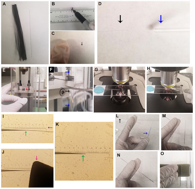
A. Cut a bundle of carbon fiber to a slightly longer length than a capillary tube. B. Marking the center point of a capillary tube is helpful for placement into the gravity electrode puller (see Figure 1E). C. While wearing gloves, isolate a single carbon fiber, and gently restrain one end of the fiber with a finger. D. Affix a capillary tube in the house vacuum line (blue arrow), and, while holding one end of the carbon fiber, suction the other end of the carbon fiber (black arrow) into the capillary tube. E. Load the capillary tube containing a single carbon fiber into the gravity electrode puller, and position the center point of the capillary tube in the heating element (red arrow). F. Upon completion of electrode pulling, cut the carbon fiber (black arrow) connecting the two electrodes (blue arrows) with scissors, to create two CFEs. G. Using a light microscope with a reticle and a 10x objective, position the CFE on a slide with the tip touching the glass slide (a small piece of putty may be used to prop the CFE in the correct position). H. Use a scalpel blade to cut the carbon fiber to the appropriate length. I. The uncut CFE is shown under the 10x objective. The interface between the glass and the carbon fiber is shown at the green arrow. J. Use a scalpel blade to cut the CFE to appropriate length (30-100 μm). It is very helpful to make sure the tip of the razor blade is against the slide glass and visible in the microscope for more accurate cutting (pink arrow indicates blade tip). K. CFE shown after cutting the carbon fiber, shown with glass interface indicated by the green arrow. L-N. Insertion of a stainless steel conductive wire coated with Silver Print II into CFE. L. Stainless steel wire (blue arrow) and cut CFE (black arrow). M. Coat one end of the wire and blue insulation in Silver Print II. N. Insert wire into CFE. O. Completed CFEs should be left in a fume hood to dry for at least 12 h prior to use; store in a plastic box with foam to hold the CFE, as shown.

1. Setting up

   1. Prepare fresh ACSF solution and aliquot to the approximate volumes noted below:

      1. 200 ml into the bottle containing frozen ACSF (described above), to be used for slice preparation (referred to as bottle 1a).

      2. 500 ml into a cylinder for each FSCV rig, to be used during experiment (additional ACSF may be needed for longer experiments) (referred to as cylinder 1b).

      3. 200 ml into a storage beaker with netted wells to retain extra slices, to be oxygenated and maintained at room temperature (referred to as storage beaker).

   2. Oxygenate prepared ACSF (a-c listed above) by turning on the gas regulator of the carbogen tank, and place a gas dispersion tube into each container. Oxygen should flow continuously, and a steady stream of bubbles should be observed.

      Note: Take care not to over-oxygenate, which has the appearance of vigorous or rolling bubbles.

   3. Place the vibratome stage and brain matrix (Figure 1A) in the freezer at -20 °C, and add a fresh blade to the vibratome; set the thickness and slicing speed (mouse–speed 0.46 mm/sec and thickness 300 μm; rat–speed 0.60 mm/sec and thickness 400 μm).

   4. Prepare the FSCV rigs by adding deionized water to fill the bottom portion of the recording dish.

      Note: Ensure that water is covering the heater coil to prevent melting of tubing.

   5. Flow oxygenated ACSF from cylinder 1b into the slice well at 1 ml/min by using a peristaltic pump or gravity flow with a Control-A-Flo Regulator.

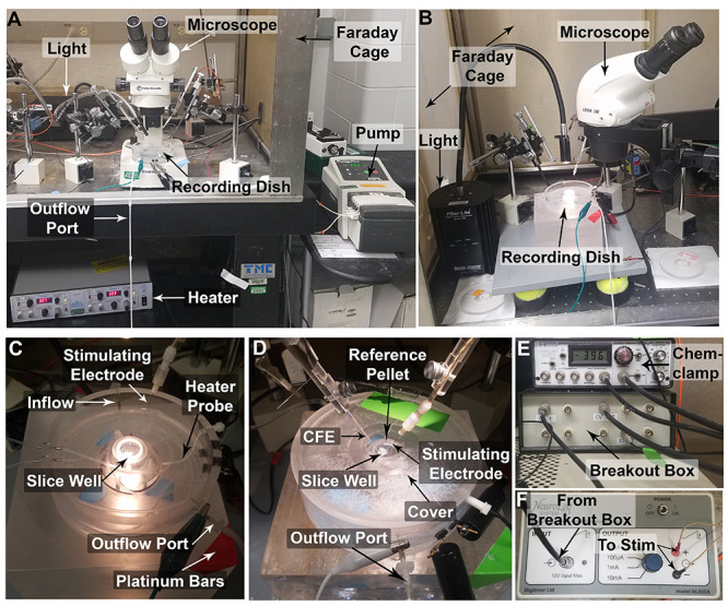
   6. Turn on the following equipment: (1) temperature controller TC-344C, set to 32 °C in the recording dish; (2) Current Stimulus Isolator, output set to 1 mA; (3) Chem-Clamp; (4) light source, and (5) microscope (visualized in Figures 3A-3B).

   7. Draw fluid from the recording dish’s outflow tubing using a syringe, which will allow fluid to start flowing out of the dish and into the waste bottle.

      Note: Throughout experimentation, outflow needs to be maintained. This can be particularly troublesome with new tubing, which may require the outflow to be reestablished several times throughout the day.

   8. Before brain extraction, add ~50 ml of the cold, oxygenated ACSF from bottle 1a to cylinder 1b containing frozen ACSF. This will be used for transporting the brain to the vibratome.

2. Brain extraction (refer to Papouin and Haydon [2018] for further details)

   1. Add isoflurane to an induction chamber, and allow the gas to disburse throughout the chamber (2-3 min for mice; 5-10 min for rats.).

   2. Deeply anesthetize the rodent in the induction chamber, followed by immediate decapitation.

      Note: It is important to make sure the animal is still breathing (at a depressed rate) prior to decapitation. In our laboratory, rat and mouse decapitation occurs via guillotine.

   3. Expose the skull by making a midline incision (caudal to rostral) with scissors; pull the skin laterally to visualize the suture lines of the skull.

   4. Use rongeurs (for rats) or small scissors (for mice) to carefully remove the skull to expose the dorsal surface of the brain.

   5. Peel away surface blood vessels and meninges.

   6. Carefully run a spatula under the brain to free it from any cranial nerves.

   7. Once free, completely submerge the brain in cylinder 1b containing frozen and fresh ACSF.

3. Brain slicing

   1. Use forceps to transfer the brain from cylinder 1b to the brain matrix, arranging the brain ventral side up. Use a plastic pipette to transfer chilled, oxygenated ACSF (approximately 2 ml) to the brain matrix.

      Note: The brain does not have to be fully submerged at this step. Addition of ACSF onto the brain while it is in the matrix will help straighten the brain and prevent it from sticking to the surface of the matrix.

   2. While still covered in paper, snap a Personna double-edged blade into two single edge blades.

   3. Place a single edge blade at the desired location(s) in the matrix to remove excess brain tissue (referred to below as blocking) (Figure 2A).

      Note: When our group isolates slices containing the nucleus accumbens, we block caudally at the level of the hindbrain to remove the cerebellum, and block rostrally to remove the olfactory bulb and early prefrontal cortex. Take care not to block off too much tissue, preserving the desired area of interest.

   4. Place a small amount (approximately one drop) of Loctite^® 404^TM glue onto the stage, and use forceps to transfer the brain from the matrix to the stage. Quickly position the caudal side of the brain onto the glue (Figure 2B).

      Note: Be careful not to use too much glue. Overuse of glue can cause the brain to detach from the stage when ACSF is added, which will result in poor slicing conditions.

   5. Carefully push a single edge blade down the midline (dorsal to ventral) to hemisect the brain.

   6. Place the stage onto the vibratome, and fill the stage with ice-cold, oxygenated ACSF (from bottle 1a) to submerge the brain.

      Note: Avoid pouring ACSF directly onto the brain, as this could cause the brain to detach from the stage.

   7. Lower the blade into the ACSF solution, and set the slicing window to at least 1 mm beyond the dorsal and ventral ends of the brain; slice the brain at the suggested settings listed above.

   8. Using a transfer pipette or a spatula, transfer slices to slice wells of the recording dish (Figure 2C).

      Note: Extra slices can be stored in the storage beaker (Figure 2F), for up to 6 h. This storage beaker should be filled with ACSF, with continuous oxygen flow via gas dispersion tube. If needing to transfer a slice from the storage beaker to a slice well (in a recording dish), use Step C8 as noted above. Please refer to Papouin and Haydon (2018) to create the storage beaker (nest beaker).

4. Setup of FSCV equipment

   1. To weigh down the brain slice, place platinum wires at the edges of the slice distant from the recording location (Figure 2D).

      Note: Typical equipment setup for FSCV is shown in Figure 3.

   2. Place the cover onto the recording dish, and fully submerge the Ag/AgCl reference electrode pellet into ACSF solution. Use alligator clips to connect the reference electrode and the carbon fiber electrode to the headstage (Figure 3D).

   3. Prior to beginning experimentation, use an insulin syringe 28 Gauge to carefully remove any bubbles that have formed under the netting of the slice well.

      Note: It may be necessary to remove bubbles during experimentation if they affect the signal (see Note 6).

5. Setup of software (Demon Voltammetry and Analysis) for Measuring Dopamine

   1. Click Edit CV and Stim, which will allow the command voltage and stimulation settings to be set.

   2. Click Apply once parameters are set. Standard settings are shown in (Figure 4).

6. Electrode conditioning (for new electrodes only)

   1. Using a micromanipulator, lower the carbon fiber electrode to submerge the carbon fiber tip into ACSF (do not lower the carbon fiber electrode into the brain).

   2. Turn on the CV, and repeatedly scan at a frequency of 60 Hz for at least 20 min.

   3. After the above conditioning step, turn off the CV and change the frequency to 10 Hz (the working cyclic voltammetry frequency for FSCV).

      Note: Electrodes can be used 2-4 times, and this conditioning step is only required for the first use. If the electrode is not new, start at the working cyclic voltammetry frequency of 10 Hz and skip to collecting dopamine signals. The conditioning step allows stabilization of new electrodes to occur quicker.

7. Collecting dopamine signals

   1. Using a micromanipulator, lower the carbon fiber electrode approximately 75 µm (visual estimation) into the brain region of interest.

   2. Lower the bipolar stimulating electrode (using a micromanipulator) onto the surface of the slice, 100-200 µm from the carbon fiber electrode (Figure 1E).

      Note: A common early mistake is puncturing the surface of the slice when lowering the stimulating electrode. It is helpful to slowly lower the stimulating electrode until the surface of the slice dimples. When the dimpling effect occurs, slightly elevate the stimulating electrode to ensure it rests on top of the slice surface.

   3. Name the collection files and set the save folder.

   4. Set the number of collection files to 1, and uncheck the “Wait” button. The file name can be set to “default” for this step, or renamed.

      1. A few electrode placements may be needed in order to achieve an optimal signal (depicted in Figure 4).

      2. When trying to achieve an optimal signal, it is better for slice health to move the carbon fiber electrode rather than the stimulating electrode (which, due to size, can damage the tissue).

   5. Once a reasonable dopamine signal is obtained (optimally greater than 3 nA for rat slices and greater than 7 nA for mouse slices; Figure 5), set the desired number of collection files. Set the collection interval to either 180 sec (for single pulse experiments) or 300 sec (for multi-pulse experiments).

   6. Click the Collect button to begin collecting dopamine signals.

   7. Stop the collection after 30-40 min of collecting baseline signals (at least 10 collections with a 180 sec interstimulus interval or at least 8 collections with a 300 sec interstimulus interval).

   8. Click the Analyze button, and check the last three signals to see if collections have stabilized (amplitude varying less than 10% between collections, and not all increasing or decreasing. For example, if the last three collections have amplitudes of 9.8 nA, 10.2 nA, and 10.5 nA, the dopamine signal is not stable. If the collections were 9.8 nA, 10.2 nA, and 9.7 nA, the signal is stable, and the experimenter can move on to step G7).

      Note: Do not let the slice sit without regular stimulation at the selected interstimulus interval, or else the signal will need to be restabilized.

   9. After stability, a pharmacological agent of interest can be added to the ACSF cylinder. Change the collection name, and collect for a minimal of 30 min to allow the pharmacological agent to reach maximal effect.

      Note: A pharmacological agent can be added at cumulative doses to create a concentration-response curve. Once the curve is complete at the desired concentrations, the experiment has ended, and the slice is no longer usable for other experimentation.

   10. Upon completion of experimentation, turn off the CV button.

   11. Disconnect the carbon fiber electrode and the stimulating electrode from the headstage.

   12. Move the carbon fiber electrode to the calibration system to determine the electrode’s sensitivity to dopamine.

       Note: It is best practice to perform calibration at the end of each experiment, or prior to using the electrode for another experiment. Even if the same electrode is used for two experiments, sensitivity to dopamine can change due to fouling of the electrode.

8. Calibration of carbon fiber electrode (Figure 6)

   1. Dilute dopamine in ACSF to a known concentration of dopamine (our laboratory uses 3 μM), and fill a 5 ml syringe with the diluted dopamine solution.

   2. Fill a 30 ml syringe with ACSF solution, and place it on a single syringe infusion pump.

   3. Open the Demon Voltammetry software and use the same settings as listed above, except change the collection interval to 0 sec and number of files to 5.

   4. Reconnect the carbon fiber electrode and reference electrode to the same headstage as the performed experiment.

   5. Run ACSF through the calibration system using the single syringe infusion pump, and lower the carbon fiber electrode into the ACSF solution (Figure 6A).

   6. Turn on the CV button (electrode signal shape should appear the same as during experimentation), and start the collection.

   7. Allow ACSF to flow for 5 sec, and then apply a consistent flow of the diluted dopamine solution for the next 5 sec, followed by ACSF solution. Continue for each additional collection.

      Note: Dopamine signal should have an approximately square-shaped peak (Figure 6B).

   8. Analyze calibration collections to ensure the dopamine signals are stable (not trending in one direction). If the dopamine current continued to increase or decrease, repeat Step H6 to collect additional calibration data.

   9. Once the dopamine signals are stable, average all of the dopamine currents (nA) collected. Divide the average current by the concentration of the dopamine solution used for calibration (3 μM) in order to determine the calibration factor (nA/μM).

      Note: If any collection amplitudes vary drastically from other collections, exclude it and average accordingly.

9. Clean up

   1. Flow a 70% Ethanol solution through each recording dish for 10 min at an increased flow rate (e.g., 2 ml/min). Repeat with 3% hydrogen peroxide, then distilled water.

   2. If using a peristaltic pump, allow air to flow through the line until all liquid has been displaced from the tubing. If using a gravity flow system, set the Control-A-Flo Regulator to the “prime” function, and use a syringe to push air through the tubing to clear out any residual liquid.

   3. Empty used ACSF into an appropriate waste container.

Figure 3. Setup of Fast Scan Cyclic Voltammetry Equipment.

A. A typical FSCV setup (referred to as FSCV rig). B. Alternate typical FSCV setup. C. Closer view of the recording dish, without the cover. D. Recording dish with cover, brain slice in slice well, and stimulating electrode and carbon fiber electrode in place. E. Amplifier (Chem-clamp) and digitizer (Breakout Box) setup. F. Stimulus generator (Neurolog) showing input from Breakout box and output to bipolar stimulating electrode.

Figure 2. Brain slicing (mouse shown).

A. Using a brain matrix, block the brain at the appropriate rostral (red arrow) and caudal (blue arrow) locations using single edge blades. B. Adhere the brain rostral side up onto the stage, hemisect, and submerge the brain in cold, oxygenated ACSF. C. Using spatula or transfer pipette (not shown), carefully transfer brain slice to recording dish (nucleus accumbens (NAc) shown in purple). D. Secure the brain slice using platinum weights, placed distally from region of interest. E. Place bipolar stimulating electrode and carbon fiber electrode in the region of interest (NAc shown). F. Diagram of storage beaker containing oxygenated ACSF with netted wells to retain slices (O₂ refers to carbogen that is flowed into the beaker via a gas dispersion tube).

Figure 4. Demon Voltammetry setup for dopamine detection.

A. User Interface showing typical experimental settings with ideal current-voltage plot from an electrode (red box). For carbon fiber electrode conditioning, the CV freq (blue box) may be increased from 10 Hz to 60 Hz. B. Command Voltage settings. Switching potential can be adjusted as needed (red box; see Note 4). C. Stimulation settings for single pulse experiments (frequency is not used for single pulses). Frequency and pulse number (red box) can be adjusted as needed for multipulse experiments (see Note 5).

Figure 6. Electrode Calibration.

A. Electrode calibration system. A pump is used to drive ACSF through a T connector with stopcock (blue arrow). Electrodes are lowered into the ACSF droplet (red arrow), and electrodes and reference wire (black arrow) are connected to the headstage. B. Ideal calibration curve showing a square shape with fast kinetics. C. Non-ideal calibration curve obtained from a “slow” electrode that has been overused. Lipids and proteins can adhere to and foul the surface of the carbon fiber following repeated usages. This slows the kinetics of dopamine detection, resulting in sloping–rather than square–calibration curves (red arrows indicate regions of slowed kinetics).

Data analysis

1. Demon voltammetry analysis with Michaelis-Menten modeling (see Yorgason et al., 2011 )

   Note: This procedure describes the Michaelis-Menten curve fitting analysis technique. However, a number of kinetic parameters can be analyzed by Demon Voltammetry and Analysis program. Please see Yorgason et al. (2011) for thorough review.

   1. Open the program and click Analyze.

   2. Click the Open File button to allow the user to choose the file of interest.

   3. Click Kinetics, and input the calculated calibration factor (nA/µM) for the experiment

   4. Go to the Baseline Correction Tab, and move the start (green) line and end (red) line to the beginning of the collected signal. Click Reset, then Pre Stim Shift. The Baseline offset should now appear as 0.00.

   5. Go to the Peak and Decay tab. Position the Pre (green) line at the start of the dopamine signal, the peak (purple) line at the peak of the signal, and the post (red) line at the end of the dopamine signal. Click Analyze, and ensure that the modeled (yellow) line appropriately fits the curve. Click Export to save the file (Figure 7A). When prompted, name the file accordingly, and select save. When saving subsequent analyses from the same experiment, you may select this file which will then retain all peak-decay data in one text file that can be tab-delimited in Excel later (see below).

   6. Go to the Michaelis-Menten Analysis tab. Enter the K_m constant of 160 nM. Alter the [DAp] so that the curve matches the peak of the trace, the V_max to fit the first one-third of the descending portion of the curve. Increase the thickness until one point exactly overlays the trace on the ascending portion of the curve. Check Pearson Coefficient closeness of modeling fit, aiming for 0.95 (note that curves analyzed from experiments using drugs that decrease dopamine release will likely show poorer fit due to decreased ratio of signal:noise). Click Export to save the file (Figure 7B).

   7. When prompted, name the file accordingly (being sure to assign a name discrete from the peak-decay file), and select save. When saving subsequent analyses from the same experiment, you may select this file which will then retain all modeled data in one text file that can be tab-delimited in Excel later (see below).

2. Exporting data to Excel

   1. Open Excel, and the CYE file containing peak/decay or modeled data to export.

      Be sure to select All Files from the dropdown list in order to see the CYE file format.

   2. When the prompt appears, ensure that the Delimited option is chosen, and click Next.

   3. When the next prompt appears, ensure that the Tab option is chosen, and click Finish.

      A table containing all files from the analyzed experiment will result. It can be helpful to create a master spreadsheet containing all experimental files from a study. Values of interest can then be analyzed using statistics software, such as Prism.

Figure 7. Voltammetry analysis using Demon Software.

A. Peak-Decay analysis. Demon software will automatically attempt to fit these parameters, but may need to be corrected slightly. The green, purple, and red lines should be placed at the stimulation time point, the peak of the signal, and a time point after the signal that has returned to baseline, respectively. The yellow dots are indicative of the program’s automated peak-decay fit. B. Michaelis-Menten model fitting, showing Demon user interface for adjusting kinetic parameters to properly fit the signal.

Notes

1. Electrode placement: When placing electrodes, it is important to maintain consistency in location between experiments. Dopamine signals change not only between locations in the region of interest (for example, the core and shell of the nucleus accumbens), but also along the dorsal-ventral and rostral-caudal axes.

2. Timing of experiments: Maintaining a consistent time in the animal’s light-dark cycle is important to ensure that temporal fluctuations in dopamine levels do not confound any potential findings ( Ferris et al., 2013 ). It is also important to extract brains at the same time points post-drug in order to consistently observe the same temporally defined drug effects.

3. Competitive inhibitors of the dopamine transporter: The kinetic constant “K_m” measures the affinity of dopamine for the dopamine transporter, and has been estimated as 160 nM based on competition binding assays (previously determined; Wightman et al., 1988 ). However, FSCV can be used to measure the effect of a competitive inhibitor of the dopamine transporter (such as cocaine) on the reuptake of dopamine. In this instance, “apparent” K_m is used, which models dopamine uptake inhibition. In order to analyze experiments in which the dopamine transporter is known to be affected, set K_m to 160 nM for analysis of the baseline curve, and fit the descending portion of the curve by adjusting V_max. For curves in the presence of inhibitor, maintain V_max at the value determined in the baseline traces, and adjust K_m. Values obtained are denoted “apparent K_m” to indicate that the constant itself is not changing, but the apparent affinity of dopamine for the dopamine transporter changes with transporter inhibition. Please note that this technique of adjusting K_m only applies in the case of dopamine transporter targeted drugs, and for all other experiments K_m should be maintained at 160 nM throughout curve fitting analysis.

4. Determining the appropriate switching potential: In the Demon Collection Software, the switching potential can be adjusted as needed. For measurement of dopamine, the switching potential can vary between 1.1 V and 1.3 V. In most FSCV labs (including our own), a switching potential of 1.2 V is utilized to provide sufficient sensitivity while also preserving the integrity of the carbon fiber electrodes for 3-4 usages. Increasing the switching potential to 1.3 V increases electrode sensitivity; however, a switching potential of 1.3 V may result in electrode “drift” or continuously changing sensitivity, and thus making it necessary to replace carbon fiber electrodes more often. The switching potential can also be reduced to 1.0 or 1.1 V to decrease sensitivity. Generally, the switching potential is only reduced when an electrode begins to “limit” during the baselining portion of the experiment (Figure 5C), and new electrodes are unavailable. Upon altering the switching potential, a new baseline needs to be collected as the peak heights (in nA) of the evoked release will be altered by the changed sensitivity of the electrode. Switching potentials are specific to the species being analyzed. Here we describe guidelines for dopamine FSCV.

5. Determining frequency and number of pulses: The frequency (Hz) and number of pulses can be altered as needed, typically when examining drug or treatment effects on “phasic-like” stimulation kinetics. While the frequency setting has no effect on single pulse experiments, typical multi-pulse experiments consist of a set number of pulses (typically 5 or 10) applied for each of a number of increasing frequencies (i.e., 5, 10, 20, 40, 60, 100 Hz) with a 300 sec inter-stimulus interval (see Ferris et al. [2013] for review).

6. Troubleshooting

   1. Electrode (Table 1)

   2. Carbon fiber electrode (Figure 8)

   3. Noise: Increased signal noise is often caused by one of the following issues: noise in the electrodes (see above), static electricity from the experimenter, bubbles in the dish, or interference from outside electrical noise (so called 60 Hz noise). As discussed previously, a “noisy” electrode can be replaced. In order to prevent static electricity from the experimenter, it is good practice to touch the grounded Faraday cage prior to touching the micromanipulators or other rig components. This will eliminate any potential static electrical build-up that may occur due to clothing or general electricity in the area. Bubbles in the dish can also contribute to noise. In this case, the bubble itself can be removed as previously described. Bubble traps can also be installed to decrease the frequency of air bubbles in the tubing reaching the dish. Interference from outside electrical noise is the most common cause of spontaneous noise in signals. The origin of electrical noise can be difficult to ascertain and often arises without warning; however, precautions can be taken to ameliorate spontaneous noise. For example, dry air can increase static and thus noise, but the use of humidifiers on dry days can provide relief. Other troubleshooting options include completely enclosing the faraday cage, ensuring that the surface of the rig is free from all tools used during setup such as forceps and syringes, and turning off the lights in the rig. In general, electronic devices such as peristaltic pumps and voltammetry equipment must be kept outside of the Faraday cage to reduce noise from these devices as much as possible.

   4. Common electrode placement errors (Figure 9)

Table 1. Common electrode complications and solutions.

Complication	Solution
Noise (Figure 8A)	Seal between glass and carbon fiber is not intact. Connection from reference electrode to the headstage may be loose. Headstage malfunction.
Not Sensitive (Figure 8B)	Carbon fiber is too short.
Too Sensitive (Figure 8C)	Carbon fiber is too long (Figure 5C). Lack of seal between glass and carbon fiber.
Stimulator Artifact (Figures 8D-8F)	Carbon fiber electrode is placed too close to stimulating electrode. Stimulating electrode is not level on tissue surface.
Wide (Figure 8G)	Electrode is old (slow). Recording from shell instead of core. Heater is not on.
Lack of Waveform	Broken electrode Malfunctioning breakout box Malfunctioning headstage Malfunctioning National Instruments card

Figure 8. Common carbon fiber electrode problems.

See Table 1 for troubleshooting tips. A. Improperly grounded carbon fiber electrode (properly grounded trace shown in red). B. Carbon fiber electrode with less-than optimal sensitivity. Note the relatively flat shape indicated by the red arrow. C. Limiting (too sensitive) carbon fiber electrode. The electrode current is exceeding the maximum limit of the computer interface, resulting in loss of data. Note that the full current range has been cut off at the red arrows. D and E. Stimulator artifact separated from signal (note that decay kinetics appear slow due to the presence of 3 μM cocaine bathing the slice). D) Trace with colorplot inset depicting voltage on y-axis, time on x-axis and current in heatmap form on z-axis; see Yorgason et al. (2011) (red and white arrows indicate visual indication of spike presence on I/T plot and colorplot, respectively). E) Dot plot representation of the trace with red arrow indicating a noise spike present. F. Stimulator artifact not separated from signal with colorplot and cyclic voltammogram inset (red and white arrows indicate visual indication of spike presence on I/T plot and colorplot, respectively). Note that the peak of dopamine in the cyclic voltammogram (~7 nA) does not correspond to an apparent peak in the trace (~19 nA), another indication of potential interfering stimulator artifact. G. Wide baseline signal with colorplot inset.

Figure 9. Ideal electrode placement.

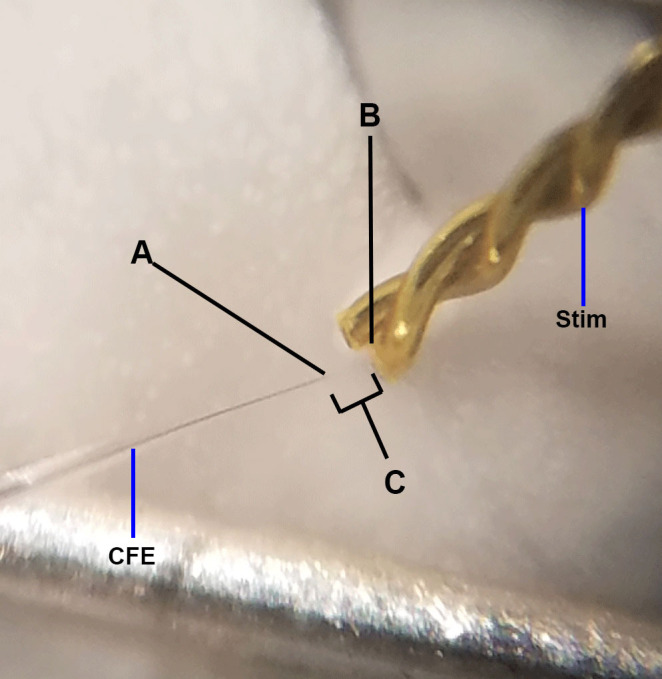
This image is adapted from Figure 1D. Above represents ideal positioning of carbon fiber electrode and bipolar stimulating electrodes (Stim) for FSCV. A. The carbon fiber electrode should be placed approximately 75 µm into the brain slice; placement too deep or too shallow will yield less-than-optimal dopamine responses. The carbon fiber electrode should also be triangulated centrally between the two stimulating wires. B. The stimulating electrode should just touch the surface of the brain; placement too deep into the tissue will result in poor FSCV signals and tissue damage. The two wires of the stimulating electrode should lie flat on the tissue; crooked stimulating electrodes can result in increased stimulation artifact observance (see Figure 5D). C. The stimulating electrode and carbon fiber electrode should be placed approximately 100-200 µm apart; placement too close together increases artifact occurrence, while placement too far apart may result in diminished dopamine signal.

Recipes

1. Artificial cerebrospinal fluid (ACSF)

   Material	Final Concentration (in mM)
   NaCl	126
   KCl	2.5
   NaH2PO4·H2O	1.2
   CaCl2·2H2O	2.4
   MgCl2·6H2O	1.2
   NaHCO3	25.0
   Ascorbic Acid	0.4
   D-Glucose	11.0
   Store at 4 °C for up to 1 day
   Use deionized water to prepare the solution

2. 10x Krebs stock solution

   Material	Final Concentration (in mM)
   NaCl	1259.4
   KCl	24.95
   NaH2PO4·H2O	12.03
   CaCl2·2H2O	8.16
   MgCl2·6 H2O	12.0
   Store at 4 °C for up to 1 month
   Use ultrapure water to prepare the solution

   Notes:

   1. 10x Krebs Stock Solution is used for preparing Artificial Cerebrospinal Fluid (ACSF).

   2. A 10x Krebs stock solution, containing the majority of solutes above (with the exception of those, NaHCO₃, ascorbic acid, and D-glucose) is prepared in advance.

3. 1 mM dopamine stock solution

   Material	Amount
   DA hydrochloride	9.4 mg
   HClO4	500 µl
   Ultrapure water	50 ml
   Store at 4 °C for up to 6 months

   On each day of experimentation, make a 3 µM solution of dopamine that will be used for calibration. For example, add 150 µl of the dopamine stock solution to 50 ml of ACSF.

Competing interests

The authors declare no competing financial interests.

Ethics

Experimental protocols adhered to National Institutes of Health Animal Care guidelines and were approved by the Wake Forest University Institutional Animal Care and Use Committee.

References

- 1. Adams R. N.(1976). Probing brain chemistry with electroanalytical techniques. Anal Chem 48(14): 1126A-1138A. [DOI] [PubMed] [Google Scholar]
- 2. Bard A. J. and Zoski C. G.(2000). Voltammetry retrospective. Anal Chem 72(9): 346A-352A. [DOI] [PubMed] [Google Scholar]
- 3. Bucher E. S. and Wightman R. M.(2015). Electrochemical analysis of neurotransmitters. Annu Rev Anal Chem(Palo Alto Calif) 8: 239-261. [DOI] [PMC free article] [PubMed] [Google Scholar]
- 4. Ferris M. J., Calipari E. S., Yorgason J. T. and Jones S. R.(2013). Examining the complex regulation and drug-induced plasticity of dopamine release and uptake using voltammetry in brain slices. ACS Chem Neurosci 4(5): 693-703. [DOI] [PMC free article] [PubMed] [Google Scholar]
- 5. Fortin S. M., Cone J. J., Ng-Evans S., McCutcheon J. E. and Roitman M. F.(2015). Sampling phasic dopamine signaling with fast-scan cyclic voltammetry in awake, behaving rats. Curr Protoc Neurosci 70: 7.. 25. 21-20. [DOI] [PMC free article] [PubMed] [Google Scholar]
- 6. Heyrovsky J.(2012).[Reproduction of: J. Heyrovsky, Chemicke Listy 1922, 16, 256-264]. Chem Rec 12(1): 17-25. [DOI] [PubMed] [Google Scholar]
- 7. Kishida K. T., Saez I., Lohrenz T., Witcher M. R., Laxton A. W., Tatter S. B., White J. P., Ellis T. L., Phillips P. E. and Montague P. R.(2016). Subsecond dopamine fluctuations in human striatum encode superposed error signals about actual and counterfactual reward. Proc Natl Acad Sci U S A 113(1): 200-205. [DOI] [PMC free article] [PubMed] [Google Scholar]
- 8. Lohrenz T., Kishida K. T. and Montague P. R.(2016). BOLD and its connection to dopamine release in human striatum: a cross-cohort comparison. Philos Trans R Soc Lond B Biol Sci 371(1705): 20150352. [DOI] [PMC free article] [PubMed] [Google Scholar]
- 9. Maina F. K., Khalid M., Apawu A. K. and Mathews T. A.(2012). Presynaptic dopamine dynamics in striatal brain slices with fast-scan cyclic voltammetry. J Vis Exp(59): 3464. [DOI] [PMC free article] [PubMed] [Google Scholar]
- 10. Papouin T. and Haydon P. G.(2018). Obtaining acute brain slices. Bio-protocol 8(2): e2699. [DOI] [PMC free article] [PubMed] [Google Scholar]
- 11. Rodeberg N. T., Sandberg S. G., Johnson J. A., Phillips P. E. and Wightman R. M.(2017). Hitchhiker's guide to voltammetry: Acute and chronic electrodes for in vivo fast-scan cyclic voltammetry . ACS Chem Neurosci 8(2): 221-234. [DOI] [PMC free article] [PubMed] [Google Scholar]
- 12. Wightman R. M., Amatore C., Engstrom R. C., Hale P. D., Kristensen E. W., Kuhr W. G. and May L. J.(1988). Real-time characterization of dopamine overflow and uptake in the rat striatum. Neuroscience 25(2): 513-523. [DOI] [PubMed] [Google Scholar]
- 13. Yorgason J. T., Espana R. A. and Jones S. R.(2011). Demon voltammetry and analysis software: analysis of cocaine-induced alterations in dopamine signaling using multiple kinetic measures. J Neurosci Methods 202(2): 158-164. [DOI] [PMC free article] [PubMed] [Google Scholar]