Dynamical Systems: From Classical Mechanics and Astronomy to Modern Methods

Abstract

We describe topological dynamics over a space by starting from a simple ODE emerging out of two coupled variables. We describe the dynamics of the evolution of points in space within the deterministic and stochastic frameworks. Historically dynamical systems were associated with celestial mechanics. The core philosophies of two kinds of dynamics emerging from Poincaré and Lyapunov are described. Smale’s contributions are highlighted. Markovian models are considered. Semi-group actions are a tool in this study.

Overview

Dynamical systems arise in several practical real-world situations apart from classical physical systems like astronomy, mechanics, etc., The dynamics could be studied purely within a single variable, say a set X or between two interacting or coupled variables, say X and Y or between several interacting variables. We start from basic dynamics arising out of any arbitrary two associated variables to more complex dynamical systems.

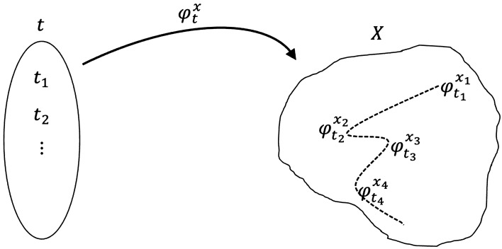
Let us consider an arbitrary space X consisting of all possible outcomes (discretely) of a random experiment. Consider a function ${\phi }_t^x$ which, for each value of t with $t\in \{t_1,t_2,\dots \},$ picks a value x for $x\in X.$ The values that the function ${\phi }_t^x$ picks and the order of the picking can be pre-arranged through a deterministic model or else the values that the function ${\phi }_t^x$ picks and order of the picking can be a random process model. A differential equation model with a parameter space $\mathrm{\Theta }$ can be employed to obtain ${\phi }_{t_i}^{x_i}(\mathrm{\Theta })$ for $i=1,2,\dots$ The complexity of the dynamics of ${\phi }_t^x$ could depend on X alone as the parameter space, say, ${\mathrm{\Theta }}_X$ describing the changes attributed to X alone, or the complexity could depend on some external spaces, say, Y, Z, W,  etc. Classical mechanics models do not capture much complexity and hence the assumptions on ${\mathrm{\Theta }}_X$ are straightforward. The parameter spaces describing the dynamics alone corresponding to the spaces Y, Z, W,  could be ${\mathrm{\Theta }}_Y,{\mathrm{\Theta }}_Z,{\mathrm{\Theta }}_W$. The points or values within the space X can be imagined as states in X. Thus the transformation from ${\phi }_{t_i}^{x_i}(\mathrm{\Theta })$ to ${\phi }_{t_{i+1}}^{x_{i+1}}(\mathrm{\Theta })$ can be treated as a change in the state within the time-step $t_{i+1}-t_i$ by the dynamical system with the base space X. These transformations which form a semigroup determine the overall system dynamics (see Fig. 1). The quantity $t_{i+1}-t_i$ is greater than zero and it could be the same for each i, $i=1,2,\dots$, or it could be different. When the outputs of ${\phi }_t^x$ result from a differential equation model, then $t_{i+1}-t_i$ is usually constant for all i values.

Figure 1:

The dynamics in the space X due to transformations ${\phi }_t^x$. External factors outside space X are not influencing the dynamics. When a dynamical system is built using the availability of points within a space X to understand the mapping of ${\phi }_t^x$ into a space X, then such a system cannot be influenced by external factors outside the space X.

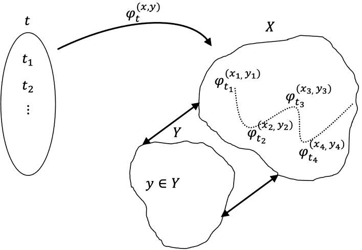
When the dynamics within the base space X are influenced by another space Y, the resultant dynamics, say ${\phi }_t^{(x,y)}$, could be different from ${\phi }_t^x$ (see Fig. 2). Suppose there is another space Y that has some influence over the values that the function ${\phi }_t^x$ picks. Later in this section, we have mentioned a classical pendulum example where the space Y we have indicated as a magnetic field. Here $Y\ne \varphi$ (empty set) and Y could be a single space or the union of a collection of spaces. Instead of ${\phi }_t^x$, we write the function ${\phi }_t^{(x,y)}$ for $x\in$ X and $y\in Y$. Let the corresponding parameter space be ${\mathrm{\Theta }}_{\mathit{XY}}$. Both the functions ${\phi }_t^x$ and ${\phi }_t^{(x,y)}$ map from the same domain to space X, i.e. ${\phi }_t^x:t\to X$ and ${\phi }_t^{(x,y)}:t\to X$ but for ${\mathrm{\Theta }}_X\ne {\mathrm{\Theta }}_{\mathit{XY}}$ the values to which ${\phi }_t^x$ picks values in X under ${\mathrm{\Theta }}_X$ are different from the values which ${\phi }_t^{(x,y)}$ picks in X under ${\mathrm{\Theta }}_{\mathit{XY}}$. The sequence of values generated under the transformation ${\phi }_t^x$ is $\{{\phi }_{t_1}^{x_1},{\phi }_{t_2}^{x_2},\dots \}$ and the sequence of values generated under the transformation ${\phi }_t^{(x,y)}$ is $\{{\phi }_{t_1}^{(x_1,y_1)},{\phi }_{t_2}^{(x_2,y_2)},\dots \}$. The order of the values picked by ${\phi }_t^{(x,y)}$ is assumed different from the order of the values picked by ${\phi }_t^x$. The mapping rules to pick values by the functions ${\phi }_t^x$ and ${\phi }_t^{(x,y)}$ can be either prefixed (deterministic framework) as mentioned above or the values that these functions will pick in X could be outcomes of a stochastic framework which we discuss below. An order of picking rules could be different for different systems under study. Under the deterministic framework, if there is no influence of Y, then we can represent the dynamics created by ${\phi }_t^x$ by

$$\begin{array}{c}\hfill \dot{X}=\phi \left({\mathrm{\Theta }}_X,,,X\right),\end{array}$$ 1.1

and if there is influence by Y then we can represent the dynamics created by ${\phi }_t^{(x,y)}$ by

$$\begin{array}{c}\hfill \dot{X}=\phi \left({\mathrm{\Theta }}_{\mathit{XY}},,,X,,,Y\right).\end{array}$$ 1.2

The value of ${\phi }_t^{(x,y)}$ at the time step $t_{i+1}$ will depend on the values of ${\phi }_t^{(x,y)}$ and ${\mathrm{\Theta }}_{\mathit{XY}}$ but not on the value of the function that was obtained at $t_{i-1}$ for $i=1,2,\dots$. This kind of data dependency only on the recent past, when blended with some probabilistic features, is known as the Markovian property. The initial value of the state X, say, ${\phi }_{t_0}^{(x,y)}$ and a parameter space ${\mathrm{\Theta }}_{\mathit{XY}}$ produce a unique combination of the sequence of functional values ${({\phi }_t^{(x,y)})}_{t>0}$ or produce a trajectory

$$\begin{array}{c}\hfill {\phi }_{t_0}^{(x,y)}\to {\phi }_{t_1}^{(x,y)}\to {\phi }_{t_2}^{(x,y)}\to \cdots .\end{array}$$

Unless the initial combinations of states and parameter spaces are perturbed, the systems (1.1) and (1.2) will always generate exactly the same dynamics over time t. Such exactness of the path or trajectories in deterministic systems guides several real-world situations, for example, designing space craft, satellites, predicting orbital paths, etc. The properties of stability of such deterministic systems are relatively easy to obtain and also to verify if there exists stability (for example, see1). In the present context, the idea of system stability can be explained as follows.

Figure 2:

The dynamics in the space X due to transformations ${\phi }_t^{(x,y)}$. External space Y influencing the dynamics of the base space X are not influencing the global dynamics.

Let ${\phi }_t^{(x^{\ast },y)}$ be the value of the mapping at the equilibrium point $x^{\ast }$. The system is stable if, for every $ϵ>0,$ there exists a distance functions $d_X$ in X such that

$$\begin{array}{c}\hfill d_X\left({\phi }_t^{(x^{\ast },y)},,,{\phi }_t^{(x,y)}\right)<\delta \text{for}\delta >0\end{array}$$ 1.3

and

$$\begin{array}{c}\hfill d_X\left({\phi }_t^{(x^{\ast },y)},,,{\phi }_t^{(x,y)}\right)<ϵ\text{for}t\ge t_0.\end{array}$$ 1.4

The system becomes asymptotically stable whenever

$$\begin{array}{c}\hfill d_X\left({\phi }_t^{(x^{\ast },y)},,,{\phi }_{t_0}^{(x,y)}\right)<\delta ,\end{array}$$ 1.5

implies that

$$\begin{array}{c}\hfill {\phi }_t^{(x,y)}\text{converges to}{\phi }_t^{(x^{\ast },y)}\text{as}t\to \infty .\end{array}$$ 1.6

Small perturbations will have a lesser impact on attaining stability of systems in comparison with large perturbations. Those systems which do not attain stability like complex continuous evolutionary systems are also sometimes useful. Lyapunov and Poincaré have introduced various techniques for understanding the stability of deterministic systems1^–4. We will later see that such a feature of uniqueness is not maintained under the stochastic framework.

In classical pendulum mechanics, this phenomenon of Y influencing the values ${\phi }_t^{(x,y)}$ picked from the space X can be treated as adding a magnetic field around the pendulum that influences the path of the oscillations. By changing the degree of a magnetic field the motion of a pendulum can be altered. Y acts like an external factor. In that case, ${\phi }_t^x$ has the property that the pendulum is oscillating without any external influences beyond the standard gravitational forces that affect any normal pendulum motion. Deterministic modeling equations with a predetermined $\mathrm{\Theta }$ are sufficient when practical situations like pendulum movement with factors influencing the pendulum movement are well understood. This is true even if external spaces are known to influence the location of the pendulum. The value of time could be continuous, for example, $t\in [0,\infty ).$

Under the stochastic framework, the jump from ${\phi }_{t_i}^{(x_i,y)}$ to ${\phi }_{t_{i+1}}^{(x_{i+1},y)}$ is decided by a random process model. Under this framework, let us write ${\xi }_{t_i}^{(x_i,y)}$ for the values of X under the influence of another space Y mapped at the time step $t_i$ for $i=0,1,2,\dots$. Let ${\pi }_j$ be the probability that initially the system is at the state $x_j$ for $x_j\in X$ so that ${\xi }_{t_0}^{(x_j,y)}={\pi }_j.$ A random process model will have a state space X, a random variable ($\xi$), and some governing rules to pick values according to the random variable from X. A random variable is a real-valued function whose domain $\mathrm{\Omega }$ has all possible outcomes for an experiment. The state space will consist of all possible values that ${\xi }_t^{(x,y)}$ can pick. Here t could be discrete or continuous and the state space could be discrete or continuous. Let the first value picked by ${\xi }_t^{(x,y)}$ at $t_1$ be denoted by $x_1$, so that ${\xi }_{t_1}^{(x,y)}=x_1$ for $x_1\in X;$ the second value picked by $x_i$ at $t_2$ should be denoted by $x_2$, so that ${\xi }_{t_2}^{(x,y)}=x_2$ and so on; thus let ${\xi }_{t_i}^{(x,y)}=x_i$ for $i=2,3,\dots$. After starting from $x_j$, at each time step the variable $x_i$ might pick a new state or remain at the same state. We call this a transition to a new state or remaining at the same state. This construction is reminiscent of a Turing machine.

The transitions

$$\begin{array}{c}\hfill x_j\to {\xi }_{t_1}^{(x,y)}\to {\xi }_{t_2}^{(x,y)}\to \cdots ,\end{array}$$ 1.7

might represent a constant sequence $x_j$ or a sequence of distinct states or represent a combination of distinct and constant states of X (see Fig. 1). Let $p_{x_i,x_j}$ represent the probability of transition from the state $x_i$ to the state $x_j$. Then the above transitions in (1.7) are represented by the corresponding probabilities as shown below:

$$\begin{array}{c}\hfill \begin{array}{c}{p}_{x_j,x_1}\\ \overbrace{x_j\to {\xi }_{t_1}^{(x,y)}}\end{array},\begin{array}{c}{p}_{x_1,x_2}\\ \overbrace{{\xi }_{t_1}^{(x,y)}\to {\xi }_{t_2}^{(x,y)}}\end{array},\begin{array}{c}{p}_{x_2,x_3}\\ \overbrace{{\xi }_{t_2}^{(x,y)}\to {\xi }_{t_3}^{(x,y)}}\end{array}\to \cdots .\end{array}$$ 1.8

The general questions that we ask in these frameworks are related to quantifying the probabilities of transitions between the states of X and whether the states obey recurrent or transient properties. Does there exist any periodicity for the states? What is the long-term behavior of sequences of probabilities? A state i is said to be recurrent if ${\sum }_{n=1}^{\infty }{f}_{\mathit{ii}}^{(n)}=1$, otherwise it is transient, where $f_{\mathit{ii}}^{(n)}$ denote the probability that a random variable starting from initial state i returns for the first time to state i in the nthstep. Suppose d(i) be the greatest common divisor of all integers $n\ge 1$ for which probability of transition from the state i to i is greater than zero, then the state i is said to have period d(i). The transition of ${\xi }_{t_i}^{(x,y)}$ and ${\xi }_{t_{i+1}}^{(x,y)}$ depends only on the state that the random variable associated with the process picks at time $t_i$ for all $i=1,2,\dots$. Then we say that the system of random variables obeys the Markov property5^,6.

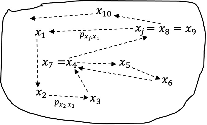
When all the states of X are recurrent, and each can be reached by the other states (either directly or indirectly) as shown in Fig. 3, and there is a unique invariant distribution $\pi$ such that $\pi =pP,$ where $P={(p_{x_i{x}_j})}_{\mathit{ij}}$ is the transition probability matrix, then

$$\begin{array}{c}\hfill \underset{n\to }{lim}\pi p_{x_i{x}_j}^{(n)}={\pi }_{x_j}.\end{array}$$

One of the key differences between dynamics due to Lyapunov and the dynamics in the stochastic framework is that, in the former, the trajectories created by a set of initial values will be unique. But, in the latter framework, the path connecting states in X created by the same starting state $x_j$ for $x_j\in X$ need not be unique. This distinction between the two kinds of philosophies challenges the Lyapunov dynamical systems usage in randomly evolving natural phenomena, like genetic or parasite evolution models, etc., However, the mathematical dynamical systems have profound applications when the dynamics have minimal influence due to random events as in mechanical systems, space explorations, solar systems, etc.

Figure 3:

States in the space X under a stochastic environment. A random model could return to the same state at a different time step as shown at $x_4$, $x_7$ and at $x_j,x_8,\text{and}{x}_9$.

Proposition 1

Let $(D,{\mathrm{\Theta }}_X)$ be the differential equation-based dynamical system on a space X with parameter space ${\mathrm{\Theta }}_X$ and let ${\psi }_D$ be the set of trajectories generated by ${\mathrm{\Theta }}_X.$ Let (M, X) be the stochastic dynamics created due to the model M on the same space X. Let $p_{x_i,x_j}$ be the transition probabilities from $x_i$ to $x_j$ for all $x_i,x_j$ in X. Let $\gamma$ be the paths joining the states in X after the states are selected by the function $\xi$ with $\gamma :[t_0,t_n]\to X$, where $\gamma (t_0)=x_j$ and $\gamma (t_n)=x_n$ for $x_j,x_n\in$X. Then ${\psi }_D$ is unique on $[t_0,t_n]$ whereas $\gamma$ need not be unique.

In the next section, we will review classical dynamical systems explained by Poincaré and Lyapunov. We will discuss the topological dynamics due to Stephen Smale7 as well as ergodicity results of Katok2.

Topological Dynamics

Mathematically, topological dynamics was first studied by Henri Poincaré during the early 20th century2. Some understanding of the dynamics of celestial objects through celestial mechanics has existed as far back as ancient Indian and ancient Greek works of literature8^, 9. However, Poincaré first conceptualized the idea of topological dynamics while understanding the qualitative properties of differential equations. Among the many technicalities, the ideas of homeomorphisms, topological spaces, semigroups of continuous transformations between spaces, diffeomorphisms, flows between various states of spaces, etc., played a central role in several advancements in the field.

Several ideas of planetary motion, gravitational forces, solar system movements later termed celestial mechanics during the post-Copernican era were known to ancient Indian and Greek philosophers, astrologers, and mathematicians. For example, Aryabhatta (5th century BC) computed the number of lunar days and the value of $\pi$ using planetary movements9. Bhaskara’s 12th century AD book Siddantasiromani has descriptions of several ancient Indian computations of planetary motions9^–11. These ancient celestial mechanics combined with the modern-day understanding of such mechanics after the availability of new techniques perhaps inspired the formulation of dynamical systems, their study formally using differential equations12.

Poincaré’s 3-body approach using Newtonian type gravitational forces formed foundations for the n-body problems and qualitative understandings using dynamical systems. Kolmogorov’s and others’ ideas of chaos theory enriched the understanding of dynamical systems through ergodic properties. In the next few paragraphs, we will define and describe some of the previously mentioned technicalities.

Homeomorphic Spaces and Semigroups

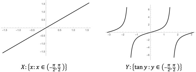
Suppose that X and Y are two topological spaces. If $f:X\to Y$ is a continuous, open, one-to-one, and onto mapping, then we say X and Y are homeomorphic. An example can be seen in Fig. 4. We consider that two spaces X and Y topologically have the same structure if they are homeomorphic. A semigroup is a set X with an associated binary operation13^–15. These semigroups are associated with transformation semigroups, say, (X, S), where S is the semigroup of transformations of X. Semigroups are associated with Markov processes on the space X5. Let us now see explicitly the association of semigroups with Markov process.

Figure 4:

A homeomorphism between two spaces X and Y on $\mathbb{R}$ with $f(x)=tanx$.

Markov Processes in Continuous Time

Let $\{X(t):t\in (0,\infty ]\}$ be a collection of discrete points or random variables $\{x_1,x_2,\dots \}$ or $\{x_1,x_2,\dots ,x_n,x_{n+1}\}.$ The stochastic process $\{X(t)\}$ is called a continuous-time Markov chain if, for any $t_1<t_2<\cdots <t_n<t_{n+1},$

$$\begin{array}{cc}\hfill \text{Prob}[X(t_{n+1})& =x_{n+1}/X(t_1)=x_1,X(t_2)=x_2,\dots ,X(t_n)=x_n].\hfill \end{array}$$ 2.1

$$\begin{array}{cc}& =\text{Prob}[X(t_{n+1})=x_{n+1}/X(t_n)=x_n].\hfill \end{array}$$ 2.2

The probability $p_{x_i,x_j}$ describing the transition from the state $x_i$ in X to the state $x_j$ in X within a time-step $t_j-t_i$ is given by

$$\begin{array}{c}\hfill p_{x_i,x_j}(t_j-t_i)=\text{Prob}[X(t_j)=x_j/X(t_i)=x_i]\text{for}{t}_i<t_j.\end{array}$$ 2.3

Such transitions (2.3) in Markov chains obey the Chapman–Kolmogorov equations (2.4)

$$\begin{array}{c}\hfill \sum _{k=0}^{\infty }{p}_{x_i,x_k}(t_k-t_i)p_{x_k,x_j}(t_j-t_k)=p_{x_i,x_j}(t_j-t_i)\text{for}{t}_i<t_k<t_j\end{array}$$ 2.4

with $t_i,t_j\in [0,\infty ).$ This implies that

$$\begin{array}{c}\hfill P(t_k-t_i)·P(t_j-t_i)=P(t_j-t_i),\end{array}$$ 2.5

where P(.) is the transition matrix of all possible transitions in the space X. We see that the semigroup property holds because of the Chapman–Kolmogorov equations satisfied by Markov chains16^–18.

Definition 2

(Semigroup)

A semigroup is a weaker structure of a group and is a set with an associative binary operation.

Definition 3

(Chapman–Kolmogorov equations) The n-step transition probability $p_{\mathit{ij}}^{(n)}$ of a discrete random variable $X_n$ describes the probability of transferring from state i to state j in n time steps. One can similarly define $p_{\mathit{ij}}^{(n-m)}$ and $p_{\mathit{ij}}^{(m)}$ to describe transitions in $(n-m)$ and m steps, respectively. For an arbitrary state k, the Chapman–Kolmogorov equations associate these transition probabilities as

$$\begin{array}{c}\hfill p_{\mathit{ij}}^{(n)}=\sum _{k=1}^{\infty }{p}_{\mathit{ik}}^{(m)}{p}_{\mathit{kj}}^{(n-m)},(0<m<n).\end{array}$$

Definition 4

(Diffeomorphisms) Let us consider two manifolds $M_1$ and $M_2$ (manifolds are a class of topological spaces). A function $f:M_1\to M_2$ is called a diffeomorphism if f is continuously differentiable, one-to-me, onto and $f^{-1}:M_2\to M_1$ is also continuously differentiable19.

Definition 5

(Flows) Let $\dot{y}=h(y)$ and $y(0)=y_0$ be the initial value problem for a vector field h(y). Saying that the function ${\varphi }_t(y)$ is the flow of h(y) means that $y(t)={\varphi }_t(x^{\ast })$ is the solution for the initial value problem.

From Poincaré to Recent Developments

One of the elementary ways of understanding the qualitative behavior of any given dynamical system, for example as in (1.1) or (1.2), is through obtaining steady-state solutions of a corresponding linearization of the given dynamical system. Poincaré in the early 20th century for such a class of systems (for celestial mechanics) showed that, if ${\phi }_t^x$ or ${\phi }_t^{(x,y)}$ is analytic at $x^{\ast }$ and if eigenvalues of $D{\phi }_t^x$ exist, then the system of equations of type (1.1) or (1.2) can be changed to a linear system2^, 12. The idea of studying the qualitative behavior of a system around the neighborhood of the equilibrium was a ground-breaking work by Poincaré and that was extended by several other researchers to a variety of situations. The behavior of the dynamical system near the hyperbolic equilibrium is equal to the behavior of the linearized system at the equilibrium point. This simplification is possible because of the Hartman–Grobman theorem20^–23. Suppose there is a hyperbolic equilibrium point $x^{\ast }$ (i.e., with nonzero real eigenvalues of $D{\phi }_t^x(x^{\ast })$) and suppose that ${\phi }_t^x$ is continuously differentiable (or $C^1$ differentiable) from a neighborhood such that the function transforms this neighborhood to a corresponding linear system.

Theorem 6

(Hartman–Grobman theorem) Let ${\mathbb{R}}^n$ be n-dimensional Euclidean space. Let $S\subset {\mathbb{R}}^n$,$x^{\ast }\in S$ and a neighborhood $B_{\delta }(x^{\ast })\subset S$ for some $\delta >0.$ Let $\phi :S\to {\mathbb{R}}^n$ be a $C^1$ function on S such that $\phi (x^{\ast })=0.$ Let $D{\phi }_t^x(x^{\ast })$ be a hyperbolic equilibrium point of the system (1.1). Then there are two open neighborhoods U (for $x^{\ast }$) and V (for 0) and a homeomorphism $H:U\to V$ such that the flow (transformation) ${\phi }_t^x$ of the system (1.1) with $X(0)=x$ a topological flow is equivalent to the flow of its linearization $e^{tD{\phi }_t^x(x^{\ast })}:$ $H({\phi }_t^x)=e^{tD{\phi }_t^x(x^{\ast })}H(x)$ for all $x\in U$ and $\left|t\right|\le 1.$

A smooth diffeomorphism $\phi$ is a topological conjugate $D\phi$ near a hyperbolic equilibrium point $x^{\ast }$ by a local homeomorphism H. As mentioned above, this theorem provides qualitative behavior around a neighborhood of the equilibrium. Because the dynamics produced by linearization are the same as the topological flow, we consider them as equivalent. Due to such equivalent nature, a given complex dynamical system is linearized to understand steady-state solutions.

What Did We Learn From Smale’s Work?

Dynamical systems development from the days of Isaac Newton to Poincaré was inspired by celestial mechanics. Such kind of dynamics if understood correctly prior to the development of mathematical formulations were less influenced by fluctuations of external forces after the initiation of the dynamics. The functions like ${\phi }_t^x$ can be built from piecewise connectedness properties.

Further mathematical developments of the dynamics by Lyapunov, Kolmogorov, Hartman, Grobman, Smale involved pure mathematical formulations. These formulations involved homeomorphisms, diffeomorphisms, and continuous transformation of open sets. Such formulations as in Poincaré do not change the course of the dynamics after initial values or initial points of reference that were set at $t_0$ or at 0. Even the global stability features that were discussed earlier or the local stability features of Hartman–Grobman were purely mathematical possibilities and would perfectly fit well for the situation as in celestial mechanics. The Hartman–Grobman type of constructions of neighborhoods $B_{\delta }(x^{\ast })\subset S$ and transformation functions like $H:U\to V$ proves that studying corresponding linearized systems are enough to understand the dynamics in a given dynamical system outside celestial mechanics. All the developments up to Smale strongly emphasize dynamical systems that are independent of unexpected influence on the solution function ${\phi }_t^x$ or any random fluctuations on ${\phi }_t^x$.

Building an analysis that is bound to give a stable equilibrium either locally or globally is relatively easier than building such an analysis for a truly unpredictable ${\phi }_t^x$ for $t>0$. Consider the function $H({\phi }_t^x)$ of the Hartman-Grobman theorem for $t\in [t_0,\infty ).$ Let there be fluctuations in the data on which the system was built after the initialization of the dynamics such that $H({\phi }_t^x)$ at $t_1\in [t_0,\infty )$ is not equal to the value of the function $H({\phi }_t^x)$ at $t_1$ i.e. $H({\phi }_{t_1}^x).$ The functional values $H({\phi }_t^x)$ for $t\in [t_0,t_1)$ trace out a set of points in V (the curve described by $H({\phi }_t^x)$ for $t\in [t_0,t_1)$). The linearized system generated by Hartman–Grobman will provide the dynamics of the system until $t_1-{ϵ}_1$ for ${ϵ}_1>0$ and fail to provide the true dynamics at $t_1.$ Let the true values of $t_1$ be the new initial value for the system. Let the function $H({\phi }_t^x)$ for the new dynamics starting from $t_1$ be plotted to get a curve $H({\phi }_t^x):[t_1,\infty )\to V.$ Suppose that $H({\phi }_t^x)$ at $t_2$ is not equal to the values of $H({\phi }_t^x):[t_1,\infty )\to V$ at $t_2$ for $t_2>t_1.$ Let the rest of all values of $H({\phi }_t^x):[t_1,t_2-{ϵ}_2)$ for ${ϵ}_2>0$ be equal to the true values for the same interval. The true values $t_2$ will be new initial values of the dynamical system. In general, let the time points at which the liniearized system values differ from the true values values be at $t_i$ for $i=1,2,\dots \infty$ and the new initial values of the function $H({\phi }_{t_{i-1}}^x)$ be used to obtain the dynamics for the period $H({\phi }_t^x):t\in [t_{i-1},t_i-{ϵ}_i)$ for $i=1,2,\dots ,$

Let

$$\begin{array}{c}\hfill {\mathrm{\Gamma }}_{t_i}={\mathrm{\Sigma }}_{i=1}^{\infty }∥H,({\phi }_{t_i}^x),-,H,({\phi }_{t_{i-1}}^x)∥\end{array}$$ 2.6

be the length of the polygon generated up until the time $t_i.$ The length of the curve generated by

$$\begin{array}{c}\hfill H({\phi }_t^x):[t_0,\infty )\to V],\end{array}$$

say $L_{t_i}$ for the time interval $[t_0,t_1)$, will be different from the polygon (2.6). Hence the original dynamics generated by $H({\phi }_t^x)$ that was obtained through the Hartman–Grobman construction will be different from ${\mathrm{\Gamma }}_t$ for $t\in [t_0,\infty ).$ The trajectories of the function $H({\phi }_t^x)$ with initial values $t_0$ will be different from the polygon that was obtained while computing the length ${\mathrm{\Gamma }}_t$ (2.6) for the same period $[t_0,\infty ).$ Suppose ${\gamma }_i$ to be the length of the polygon from $t_{i-1}$ to $t_i$ and $H({\phi }_{s_i}^x)$ to be the true value of the function at $t_i.$ Let

$$\begin{array}{c}\hfill ∥H,({\phi }_{t_i}^x),-,H,({\phi }_{s_i}^x)∥\end{array}$$

be the distance from the Hartman–Grobman constructed $H({\phi }_t^x)$ and the true value from the data at the same point.

Stephen Smale’s idea was to consider a space X with all the flows with the $C^r-$topology for $r=1,2,\dots$.7. He obtained stability of the system by considering equivalence relationships between flows and their orbit structures within the space. The flow of an ODE (ordinary differential equation) within a compact manifold gives us a closed set C for $C\in X$. The union of all the flows equals the entire space X. Let ${\psi }_{\mathit{it}}$ be the ith flow at time t. Then

$$\begin{array}{c}\hfill \bigcup _i{\int }_t{\psi }_{\mathit{it}}\mathrm{d}t=X.\end{array}$$ 2.7

The expression (2.7) can be considered as

$$\begin{array}{c}\hfill {\int }_t\bigcup _i{\psi }_{\mathit{it}}\mathrm{d}t=X.\end{array}$$ 2.8

The system of ODEs will be globally stable if, and only if, $q_{\mathit{it}}$ for each i is globally stable. There are several other kinds of dynamics and their associations with other constructions were considered, for example, associations between Hamiltonian flows, Arnol’d’s work, Narasimhan’s work, and Anosov’s diffeomorphisms7^,12^,24.

Smale’s horseshoe mapping inspired the creation of transformations of manifolds into various other forms. Smale exploited the fact that to transform a square into a horseshoe a set of points with a region of a square considered need not be disturbed. Roughly, this set of undisturbed points is associated with attractors. Such a demonstration was clever as it involved functions of continuous transformations, called attractors. Attractors are the points in the space X that are not influenced (not disturbed due to the functional transformations)25. In this famous mapping of a standard square to the shape of a horseshoe, Smale considered diffeomorphic functions that first transform a square into a strip and then stretching this strip into a horsehoe shape.

Because the diffeomorphism property was involved, the horseshoe can be reverted to the initial square.

Two Distinct Dynamics from the Same Origin

The idea of this section is to explain how the dynamics created by a system are distinct if we keep updating the system with newer information available on the trajectories. Even if these two distinct dynamical systems are generated from the same origin, we could see two or more different dynamics emerge.

Proposition 7

Suppose that $H({\phi }_{s_i}^x)$ exists for $i=1,2,3,\dots$. If ${\gamma }_i<∥H,({\phi }_{t_i}^x),-,H,({\phi }_{s_i}^x)∥$ for every i then the equilibrium analysis performed through Hartman–Grobman will not represent the true dynamics for which the dynamical system was built.

Proof

We have

$$\begin{array}{c}\hfill {\int }_0^{\infty }{\gamma }_{i}di<{\int }_0^{\infty }∥H,({\phi }_{t_i}^x),-,H,({\phi }_{s_i}^x)∥di.\end{array}$$

Here ${\gamma }_i$ is the length of the polygon from $t_{i-1}$ to $t_i$, $H({\phi }_{t_i}^x)$ is the value of the function at time $t_i,$ and $H({\phi }_{s_i}^x)$ is the true value of the function at $t_i.$ Also $H({\phi }_{s_1}^x)$ is the value in V at time $t_1$ at which the dynamics initiated at $t_0$ does not match the function $H({\phi }_t^x).$ Since $H({\phi }_{s_1}^x)$ exists and ${\gamma }_1<∥H,({\phi }_{t_1}^x),-,H,({\phi }_{s_1}^x)∥$, the path ${\gamma }_1$ in reality would not have been completed. Suppose that $H({\phi }_t^x)$ values provide the true dynamics until $t_1-{ϵ}_1$ for some ${ϵ}_1>0$. Then

$$\begin{array}{c}\hfill ∥H,({\phi }_{t_0}^x),-,H,({\phi }_{t_1-{ϵ}_1}^x)∥<{\gamma }_1,\end{array}$$

which implies that

$$\begin{array}{c}\hfill ∥H,({\phi }_{t_0}^x),-,H,({\phi }_{t_1-{ϵ}_1}^x)∥<∥H,({\phi }_{t_1}^x),-,H,({\phi }_{s_1}^x)∥.\end{array}$$ 3.1

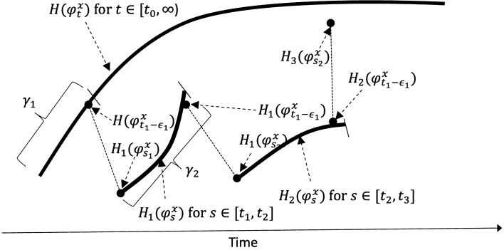
Suppose we consider the dynamics of the system with a new set of initial values as a resultant of $H({\phi }_{s_1}^x).$ There will be two sets of dynamics in the process at $t_1.$ One due to the original $H({\phi }_t^x)$ initiated at $t_0$ and continuing throughout for $t\in [t_0,\infty )$, and the second dynamic that was initiated at $t_1$ with the new set of initial values due to the function value of $H({\phi }_{s_1}^x).$ Suppose the system that was originally set is allowed to continue after $t_1$ without any interruption. The second system starting from s for $s\in [t_1,\infty )$ will have the function $H({\phi }_s^x)$ for $s\in [t_1,\infty ).$ See Fig. 5.

Figure 5:

Construction of two dynamics from the same origin.

Let us call this newer function $H_1({\phi }_s^x)$ for $H_1:U\to V_1$ and $V_1\in {\mathbb{R}}^n.$ Note that

$$\begin{array}{c}\hfill V_1\cap V=\varphi \text{or}{V}_1\cap V\ne \varphi .\end{array}$$ 3.2

We allow either of the possibilities of (3.2) in our construction.

Suppose at $t_2$ the function $H_1({\phi }_s^x)$ fails to provide the true value that the system which was initiated at $t_1$ generates. Then

$$\begin{array}{c}\hfill ∥H_1,({\phi }_{s_1}^x),-,H_1,({\phi }_{t_2-{ϵ}_2}^x)∥<{\gamma }_2,\end{array}$$

where ${\gamma }_2$ is the length of the path of $H_1({\phi }_s^x)$ for $s\in [t_1,t_2].$ This implies that

$$\begin{array}{cc}& ∥H_1,({\phi }_{s_1}^x),-,H_1,({\phi }_{t_2-{ϵ}_2}^x)∥\hfill \\ \hfill & <∥H_1,({\phi }_s^x),-,H_2,({\phi }_{s_2}^x)∥\text{for}s\in [t_1,t_2].\hfill \end{array}$$ 3.3

In (3.3), the function $H_2:U\to V_2$ with $V_2\in {\mathbb{R}}^n.$ The set $V_2$ could satisfy one of the following possibilities:

$$\begin{array}{cc}& V_2\cap V_1\cap V=\varphi \text{or}{V}_2\cap V_1\cap V\ne \varphi \text{or}\hfill \\ \hfill & \{V_2\cap V_1\ne \varphi \text{and}{V}_2\cap V=\varphi \}\hfill \\ \hfill & \text{or}\{V_2\cap V\ne \varphi \text{and}{V}_2\cap V_1=\varphi \}\hfill \end{array}$$ 3.4

Continuing the two kinds of dynamics described above, we will arrive at

$$\begin{array}{cc}& ∥H,({\phi }_{t_0}^x),-,H,({\phi }_{t_1-{ϵ}_1}^x)∥\hfill \\ \hfill & +\sum _{i=1}^{\infty }∥H_i,({\phi }_{s_i}^x),-,H_i,({\phi }_{t_{1+1}-{ϵ}_{1+1}}^x)∥<{\int }_1^{\infty }{\gamma }_i\mathrm{d}i\hfill \\ \hfill & <\sum _{i=1}^{\infty }∥H_i,({\phi }_{t_{i+1}}^x),-,H_{i+1},({\phi }_{s_{1+1}}^x)∥.\hfill \end{array}$$ 3.5

The piecewise connected path of the second dynamical system is

$$\begin{array}{cc}& ∥H,({\phi }_{t_0}^x),-,H,({\phi }_{t_1-{ϵ}_1}^x)∥+\sum _{i=1}^{\infty }∥H_i,({\phi }_{s_i}^x),-,H_i,({\phi }_{t_{1+1}-{ϵ}_{1+1}}^x)∥\hfill \\ \hfill & <{\int }_1^{\infty }{\gamma }_i\mathrm{d}i\hfill \end{array}$$ 3.6

In (3.5), the function $H_i:U\to V_i$ and and $V_i\in {\mathbb{R}}^n$ for $i=2,3,\dots$. The sets $V_i$ for $i=2,3,\dots$ could satisfy one of the following possibilities:

$$\begin{array}{cc}& \bigcap _{i=1}^{\infty }{V}_i\cap V=\varphi \text{ or }\bigcap _{i=1}^{\infty }{V}_i\cap V\ne \varphi \text{ or }\hfill \\ \hfill & \{V_k\cap V_l\ne \varphi \text{for every}k\ne l\text{and}\bigcap _{i=1}^{\infty }{V}_i\cap V=\varphi \}\hfill \end{array}$$ 3.7

The dynamics created by $H({\phi }_t^x)$ and the piecewise connected path in (3.6) and the corresponding $V_i$ values within ${\mathbb{R}}^n$ form two distinct dynamics. Hence the original functional path of Hartman–Grobman-generated dynamics would not be valid in the situation described in the proposition. $\square$

Remark 8

The result with two kinds of dynamics can be extended with multiple dynamics evolving in the space X by continuing $H_1({\phi }_s^x)$ beyond $t_2$, $H_2({\phi }_s^x)$ beyond $t_3$, and so on. This will lead to multiple dynamics within the same space X.

Remark 9

When ${\gamma }_i>∥H,({\phi }_{t_i}^x),-,H,({\phi }_{s_i}^x)∥$, we are not sure if the two dynamics created in Proposition 7 are significantly different.

Discussion

Dynamical systems, especially the topological dynamics combined with the stochastic paradigm, are a fascinating field. After Poincaré’s groundbreaking work followed by Lyapunov’s global stability analysis, works of Kolmogorov, Arnol’d, Moser, to Smale’s differential manifolds, the subject has seen expansions to applications to natural sciences26.

We have presented a new result (Proposition 1) that provides possibly a new insight into topological and stochastic dynamics within a space X and then proved a result (Proposition 7) by considering two dynamics that have started at the same time 0 or $t_0$. We are not providing proof of this proposition in this article.

Concluding Remarks

Dynamical system has grown in recent years into a powerful tool that can give new insights into geometry, differential equations, evolution theory, fractal geometry, and many other parts of modern mathematics. We have endeavored here to show how the dynamical systems point of view can shed light on questions arising from population dynamics. In particular, the Hartman-Grobman theorem gives us a handle on normalizing a dynamical system near a hyperbolic equilibrium point and then engaging in further, more detailed analysis.

What we have presented here are the only first steps in this program. We hope in future work to develop the ideas to a peak of real insight.

Biographies

Arni S.R. Srinivasa Rao

was born and raised in India until he obtained his PhD. He is a Professor and Director of Laboratory for Theory and Mathematical Modeling, Medical College of Georgia, Augusta, U.S.A. Until 2012, he held a permanent faculty position at Indian Statistical Institute, Kolkata. He conducted research and/or taught at several institutions, such as the Indian Statistical Institute, Indian Institute of Science, University of Oxford, and the University of Guelph. He taught courses such as real analysis, complex analysis, differential equations, mathematical biology, demography, and stochastic processes. His works on blockchain technology with hybrid models, epidemiological policies, and Chicken Walk Models are widely discussed for their practical value. Rao’s other noted contributions include his Partition Theorem in Populations, fundamental theorem in stationary population models (Rao-Carey Theorem), and AI Model for COVID-19 Identification.

Steven G. Krantz

was born in San Francisco, California in 1951. He received the B.A. degree from the University of California at Santa Cruz in 1971 and the Ph.D. from Princeton University in 1974. Krantz has taught at UCLA, Princeton University, Penn State, and Washington University in St. Louis. He was Chair of the latter department for five years. Krantz has had 9 Masters students and 20 Ph.D. students. He has written more than 135 books and more than 270 scholarly papers. He edits 5 journals, and is Managing Editor of 3. He is the founding editor of the Journal of Geometric Analysis. He is the creator, founder, and editor of the new journal Complex Analysis and its Synergies. Krantz has won the Chauvenet Prize, the Beckenbach Book Award, and the Kemper Prize. He was recently named to the Sequoia High School Hall of Fame.He is an AMS Fellow.

Funding

None for this work.

Availability of Data and Material (data transparency)

Not applicable.

Code Availability (software application or custom code)

Not applicable.

Declarations

Conflict of interest

None.

References

- 1.Hirsch MW, Smale S, Devaney RL (2013) Differential equations, dynamical systems, and an introduction to chaos, 3rd edn. Elsevier/Academic Press, Amsterdam, pp xiv+418 (ISBN: 978-0-12-382010-5)
- 2.Katok A, Hasselblatt B (1995) Introduction to the modern theory of dynamical systems. With a supplementary chapter by Katok and Leonardo Mendoza. Encyclopedia of Mathematics and its Applications, vol 54. Cambridge University Press, Cambridge, pp xviii+802 (ISBN: 0-521-34187-6)
- 3.Palis J Jr, de Melo W (1982) Geometric theory of dynamical systems. An introduction. Translated from the Portuguese by A. K. Manning. Springer, New York-Berlin, pp xii+198 (ISBN: 0-387-90668-1)
- 4.Nadkarni MG (2011) Spectral theory of dynamical systems. Reprint of the 1998 original. Texts and Readings in Mathematics, vol 15. Hindustan Book Agency, New Delhi, pp x+216 (ISBN: 978-93-80250-21-2)
- 5.Feller W (1971) An introduction to probability theory and its applications, vol II, 2nd edn. Wiley, New York-London-Sydney, pp xxiv+669
- 6.Bhat B (1985) Ramdas modern probability theory. An introductory textbook. Second edition. A Halsted Press Book. Wiley, New York, pp xv+270 (ISBN: 0-470-20262-9)
- 7.Smale S. Differentiable dynamical systems. Bull Am Math Soc. 1967;73:747–817. doi: 10.1090/S0002-9904-1967-11798-1. [DOI] [Google Scholar]
- 8.Sarasvati Amma TA (1979) Geometry in ancient and medieval India. With a foreword by V. Raghavan. Motilal Banarsidass, Delhi, pp xi+279 (ISBN: 0-89684-020-4)
- 9.Plofker K (2009) Mathematics in India. Princeton University Press, Princeton, pp xiv+357 (ISBN: 978-0-691-12067-6)
- 10.Krantz SG, Rao ASRS (2021) Ancient Indian mathematics needs an honorific place in modern mathematics celebration (under review)
- 11.Rakasubramaniam K, Hayashi T, Montelli C (2019) Bhāskara-prabhā. Hindustan Book Agency 2019 and Springer Nature Singapore Pte Ltd. 10.1007/978-981-13-6034-3
- 12.Arnol’d VI, Kozlov VV, Neĭshtadt AI (1988) Dynamical systems. III. Translated from the Russian by A. Iacob. Encyclopaedia of Mathematical Sciences, vol 3. Springer, Berlin, pp xiv+291 (ISBN: 3-540-17002-2)
- 13.Lang S (1965) Algebra. Addison-Wesley Publishing Co., Inc., Reading, pp xvii+508
- 14.Herstein IN (1964) Topics in algebra. Blaisdell Publishing Co. Ginn and Co., New York, pp viii+342
- 15.Fraleigh JB (1967) A first course in abstract algebra. Addison-Wesley Publishing Co., Reading, pp xvi+447
- 16.Cox DR, Miller HD (1965) The theory of stochastic processes. Wiley, New York, pp x+398
- 17.Goswami A, Rao BV (2006) A course in applied stochastic processes. Texts and Readings in Mathematics, vol 40. Hindustan Book Agency, New Delhi, pp xii+214 (ISBN: 978-81-85931-69-2, 81-85931-69-0)
- 18.Medhi J (1994) Stochastic processes, 2nd edn. Wiley, New York, pp xvi+598 (ISBN: 0-470-22053-8)
- 19.Hirsch MW (1976) Differential topology. Graduate texts in mathematics, No. 33. Springer, New York, pp x+221
- 20.Devaney RL (1992) A first course in chaotic dynamical systems. Theory and experiment. With a separately available computer disk. Addison-Wesley Studies in Nonlinearity. Addison-Wesley Publishing Company, Advanced Book Program, Reading, pp xiv+302
- 21.Krantz SG (2016) Differential equations—theory, technique, and practice with boundary value problems. Textbooks in mathematics. CRC Press, Boca Raton, pp xvi+464 (ISBN: 978-1-4987-3501-8)
- 22.Simmons GF (2017) Differential equations with applications and historical notes. Third edition [of MR0499365]. Textbooks in mathematics. CRC Press, Boca Raton, pp xxi+470 (ISBN: 978-1-4987-0259-1)
- 23.Aoki N, Hiraide K (1994) Topological theory of dynamical systems. Recent advances. North-Holland Mathematical Library, vol 52. North-Holland Publishing Co., Amsterdam, pp viii+416 (ISBN: 0-444-89917-0)
- 24.Arnol’d VI (1963) Small denominators and problems of stability of motion in classical and celestial mechanics (Russian). Uspehi Mat. Nauk 18(6):91–192
- 25.Ruelle D (2006) What is ... a strange attractor? Not Am Math Soc 53(7):764–765
- 26.Rao ASRS. Population stability and momentum. Not Am Math Soc. 2014;61(9):1062–1065. doi: 10.1090/noti1165. [DOI] [Google Scholar]
Associated Data
This section collects any data citations, data availability statements, or supplementary materials included in this article.
Data Availability Statement