Auto-G-Computation of Causal Effects on a Network

Abstract

Methods for inferring average causal effects have traditionally relied on two key assumptions: (i) the intervention received by one unit cannot causally influence the outcome of another; and (ii) units can be organized into nonoverlapping groups such that outcomes of units in separate groups are independent. In this article, we develop new statistical methods for causal inference based on a single realization of a network of connected units for which neither assumption (i) nor (ii) holds. The proposed approach allows both for arbitrary forms of interference, whereby the outcome of a unit may depend on interventions received by other units with whom a network path through connected units exists; and long range dependence, whereby outcomes for any two units likewise connected by a path in the network may be dependent. Under network versions of consistency and no unobserved confounding, inference is made tractable by an assumption that the networks outcome, treatment and covariate vectors are a single realization of a certain chain graph model. This assumption allows inferences about various network causal effects via the auto-g-computation algorithm, a network generalization of Robins’ well-known g-computation algorithm previously described for causal inference under assumptions (i) and (ii). Supplementary materials for this article are available online.

1. Introduction

Statistical methods for inferring average causal effects in a population of units have traditionally assumed (i) that the outcome of one unit cannot be influenced by an intervention received by another, also known as the no-interference assumption (Cox 1958; Rubin 1974); and (ii) that units can be organized into nonoverlapping groups, blocks or clusters such that outcomes of units in separate groups are independent and the number of groups grows with sample size. Only fairly recently has causal inference literature formally considered settings where assumption (i) does not necessarily hold (Hong and Raudenbush 2006; Sobel 2006; Rosenbaum 2007; Graham 2008; Hudgens and Halloran 2008; Tchetgen Tchetgen and VanderWeele 2012; Manski 2013).

Early work on relaxing assumption (i) considered blocks of nonoverlapping units, where assumptions (i) and (ii) held across blocks, but not necessarily within blocks. This setting is known as partial interference (Hong and Raudenbush 2006; Sobel 2006; Hudgens and Halloran 2008; Tchetgen Tchetgen and VanderWeele 2012; Ferracci, Jolivet, and van den Berg 2014; Liu and Hudgens 2014; Lundin and Karlsson 2014).

More recent literature has sought to further relax the assumption of partial interference by allowing the pattern of interference to be somewhat arbitrary (Verbitsky-Savitz and Raudenbush 2012; Liu, Hudgens, and Becker-Dreps 2016; Aronow and Samii 2017; Sofrygin and van der Laan 2017), while still restricting a unit’s set of interfering units to be a small set defined by spatial proximity or network ties, as well as severely limiting the degree of outcome dependence to facilitate inference. A separate strand of work has primarily focused on detection of specific forms of spillover effects in the context of an experimental design in which the intervention assignment process is known to the analyst (Aronow 2012; Bowers, Fredrickson, and Panagopoulos 2013; Athey, Eckles, and Imbens 2018). In much of this work, outcome dependence across units can be left fairly arbitrary, therefore relaxing (ii), without compromising validity of randomization tests for spillover effects. Similar methods for nonexperimental data, such as observational studies, are not currently available.

Another area of research which has recently received increased interest in the interference literature concerns the task of effect decomposition of the spillover effect of an intervention on an outcome known to spread over a given network into so-called contagion and infectiousness components (VanderWeele, Tchetgen Tchetgen, and Halloran 2012). The first quantifies the extent to which an intervention received by one person may prevent another person’s outcome from occurring because the intervention prevents the first from experiencing the outcome and thus somehow from transmitting it to another (VanderWeele, Tchetgen Tchetgen, and Halloran 2012; Ogburn et al. 2014; Shpitser, Tchetgen Tchetgen, and Andrews 2017). The second quantifies the extent to which even if a person experiences the outcome, the intervention may impair his or her ability to transmit the outcome to another. A prominent example of such queries corresponds to vaccine studies for an infectious disease (VanderWeele, Tchetgen Tchetgen, and Halloran 2012; Ogburn et al. 2014; Shpitser, Tchetgen Tchetgen, and Andrews 2017). In this latter strand of work, it is typically assumed that interference and outcome dependence occur only within nonoverlapping groups, and that the number of independent groups is large.

We refer the reader to Tchetgen Tchetgen and VanderWeele (2012), VanderWeele, Tchetgen Tchetgen, and Halloran (2014), and Halloran and Hudgens (2016) for extensive overviews of the fast growing literature on interference and spillover effects.

An important gap remains in the current literature: no general approach exists which can be used to facilitate the evaluation of spillover effects on a single network in settings where treatment outcome relationships are confounded, unit interference may be due not only to immediate network ties but also from indirect connections (friend of a friend, and so on) in a network, and nontrivial dependence between outcomes may exist for units connected via long range indirect relationships in a network.

The current article aims to fill this important gap in the literature. Specifically, in this article, the outcome experienced by a given unit could in principle be influenced by an intervention received by a unit with whom no direct network tie exists, provided there is a path of connected units linking the two. Furthermore, the approach developed in this article respects a fundamental feature of outcomes measured on a network, by allowing for an association of outcomes for any two units connected by a path on the network. Although network causal effects are shown to in principle be nonparametrically identified by a network version of the g-formula (Robins 1986) under standard assumptions of consistency and no unmeasured confounding adapted to the network setting, statistical inference is however intractable given the single realization of data observed on the network and lack of partial interference assumption. Nonetheless, progress is made by an assumption that network data admit a representation as a graphical model corresponding to chain graphs (Lauritzen and Richardson 2002). This graphical representation of network data generalizes that introduced in Shpitser, Tchetgen Tchetgen, and Andrews (2017) for the purpose of interrogating causal effects under partial interference and it is particularly fruitful in the setting of a single network as it implies, under fairly mild positivity conditions, that the outcomes observed on the network may be viewed as a single realization of a certain conditional Markov random field (MRF); and that the set of confounders likewise constitute a single realization of an MRF. By leveraging the local Markov property associated with the resulting chain graph which we encode in nonlattice versions of Besag’s auto-models (Besag 1974), we develop a certain Gibbs sampling algorithm which we call the auto-g-computation algorithm as a general approach to evaluate network effects such as direct and spillover effects. Furthermore, we describe corresponding statistical techniques to draw inference which appropriately account for interference and complex outcome dependence across the network. Auto-g-computation may be viewed as a network generalization of Robins’ well-known g-computation algorithm previously described for causal inference under no-interference and independent and identically distributed (iid) data (Robins 1986). We also note that while MRFs have a longstanding history as models for network data starting with Besag (1974) (see also Kolaczyk and Csárdi (2014) for a textbook treatment and summary of this literature), a general chain graph representation of network data appears not to have previously been used in the context of interference and this article appears to be the first instance of their use in conjunction with g-computation in a formal counterfactual framework for inferring causal effects from observational network data.

Ogburn et al. (2017) recently proposed in parallel to this work, an alternative approach for evaluating causal effects on a single realization of a network, which is based on traditional causal directed acyclic graphs (DAGs) and their algebraic representation as causal structural equation models. As discussed in Lauritzen and Richardson (2002), such alternative representation as a DAG will generally be incompatible with our chain graph representation and therefore the respective contribution of these two manuscripts present little to no overlap. Specifically, similar to our setting, Ogburn et al. (2017) allowed for a single realization of the network which is fully observed; however, they assume (i) an underlying nonparametric structural equation model with independent error terms (Pearl 2000) compatible with a certain DAG generated the network data. This assumption implies a large number of cross-world counterfactual independences which are largely unnecessary for identification but inherent to their model (Richardson and Robins 2013). Furthermore, (ii) their approach precludes any dependence between outcomes not directly connected on the network nor does it allow for interference between units which are not network ties. Finally, (iii) inferences are primarily based on an assumption that outcome errors for the network are conditionally independent given baseline characteristics. Our proposed approach does not require any of assumptions (i)–(iii).

The remainder of this article is organized as follows. In Section 2, we present notation used throughout. In Section 3, we review notions of direct and spillover effects which arise in the presence of interference. In this same section, we review sufficient conditions for identification of network causal effects by a network version of the g-formula, assuming the knowledge of the observed data distribution, or (alternatively) infinitely many realizations from this distribution. We then argue that the network g-formula cannot be empirically identified nonparametrically in more realistic settings where a single realization of the network is observed. To remedy this difficulty, we leverage information encoding network ties (which we assume is both available and accurate) to obtain a chain graph representation of observed variables for units of the network. This chain graph is then shown to induce conditional independences which allow versions of coding and pseudo maximum likelihood estimators due to Besag (1974) to be used to make inferences about the parameters of the joint distribution of the observed data sample. These estimators are described in Section 4, for parametric auto-models of Besag (1974). The resulting parameterization is then used to make inferences about network causal effects via a specialized Gibbs sampling algorithm we have called the auto-g-computation algorithm, also described in Section 4. In Section 5, we describe results from a simulation study evaluating the performance of the proposed approach. A data application illustrating auto-g-computation of direct and spillover effects of past incarceration on HIV/STI/HCV infection in a network of sexual and injection drug use partners is reported in Section 6. Finally, in Section 7, we offer some concluding remarks and directions for future research.

2. Notation and Definitions

2.1. Preliminaries

Suppose one has observed data on a population of N interconnected units. Specifically, for each i ∈ {1, … ,N} one has observed (A_i, Y_i), where A_i denotes the binary treatment or intervention received by unit i, and Y_i is the corresponding outcome. Let A ≡ (A₁, … ,A_N) denote the vector of treatments all individuals received, which takes values in the set {0, 1}^N, and A_−j ≡ (A₁, … ,A_N)\A_j ≡ (A₁, … , A_j−1, A_j+1, … ,A_N) denote the N − 1 subvector of A with the jth entry deleted. In general, for any vector X = (X_i, … , X_N), X_−j = (X₁, … , X_N)\X_j = (X₁, … , X_j−1, X_j+1, … , X_N). Likewise if X_i = (X_1,i, … , X_p,i) is a vector with p components, X_\s,I = (X_1,i, … , X_s−1,i, X_s+1,i, … , X_p,i). Following Sobel (2006) and Hudgens and Halloran (2008), we refer to A as an intervention, treatment or allocation program, to distinguish it from the individual treatment A_i. Furthermore, for n = 1, 2, … , we define $\mathcal{A}(n)$ as the set of vectors of possible treatment allocations of length n; for instance $\mathcal{A}(2)\equiv \{(0,0),(0,1),(1,0),(1,1)\}$. Therefore, A takes one of 2^N possible values in $\mathcal{A}(N)$, while A_−j takes values in $\mathcal{A}(N-1)$ for all j.

As standard in causal inference, we assume the existence of counterfactual (potential outcome) data $Y(\cdot )=\{Y_i(a):a\in \mathcal{A}(N)\}$ where Y(a) = {Y₁ (a), … , Y_N(a)}, Y_i (a) is unit i’s response under treatment allocation a; and that the observed outcome Y_i for unit i is equal to his counterfactual outcome Y_i (A) under the realized treatment allocation A; more formally, we assume the network version of the consistency assumption:

$$Y(A)=Y\text{ a.e.}$$ (1)

Notation for the random variable Y_i(a) makes explicit the possibility of the potential outcome for unit i depending on treatment values of other units, that is the possibility of interference. The standard no-interference assumption (Cox 1958; Rubin 1974) made in the causal inference literature, namely that for all j if a and a′ are such that $a_j=a_j^{\prime }$ then Y_j (a) = Y_j (a′) a.e., implies that the counterfactual outcomes for individual j can be written in a simplified form as {Y_j (a) : a ∈, {0, 1}}. The partial interference assumption (Sobel 2006; Hudgens and Halloran 2008; Tchetgen Tchetgen and VanderWeele 2012), which weakens the no-interference assumption, assumes that the N units can be partitioned into K blocks of units, such that interference may occur within a block but not between blocks. Under partial interference, Y_i (a) = Y_i (a′) a.s. only if $a_j=a_j^{\prime }$ for all j in the same block as unit i. The assumption of partial interference is particularly appropriate when the observed blocks are well separated by space or time such as in certain group randomized studies in the social sciences, or community-randomized vaccine trials. Aronow and Samii (2017) relaxed the requirement of nonoverlapping blocks, and allowed for more complex patterns of interference across the network. Obtaining identification required a priori knowledge of the “interference set,” that is for each unit i, the knowledge of the set of units $\left\{j:Y_i(a)\ne Y_i\left(a^{\prime }\right)\text{ a.s. if }{a}_k=a_k^{\prime }\text{ and }{a}_j\ne a_j^{\prime }\text{ for all }k\ne j\right\}$. In addition, the number of units interfering with any given unit had to be negligible relative to the size of the network. See Liu, Hudgens, and Becker-Dreps (2016) for closely related assumptions.

In contrast to existing approaches, our approach allows full rather than partial interference in settings where treatments are also not necessarily randomly assigned. The assumptions that we make can be separated into two parts: network versions of standard causal inference assumptions, given below, and independence restrictions placed on the observed data distribution which can be described by a graphical model, described in more detail later.

We assume that for each $a\in \mathcal{A}(N)$ the vector of potential outcomes Y(a) is a single realization of a random field. In addition to treatment and outcome data, we suppose that one has also observed a realization of a (multivariate) random field L = (L₁, … , L_N), where L_i denotes pretreatment covariates for unit i. For identification purposes, we take advantage of a network version of the conditional ignorability assumption about treatment allocation which is analogous to the standard assumption often made in causal inference settings; specifically, we assume that:

$$A⫫Y(a)\mid L\text{ for all }a\in \mathcal{A}(N).$$ (2)

This assumption basically states that all relevant information used in generating the treatment allocation whether by a researcher in an experiment or by “nature” in an observational setting, is contained in L. Network ignorability can be enforced in an experimental design where treatment allocation is under the researcher’s control. On the other hand, the assumption cannot be ensured to hold in an observational study since treatment allocation is no longer under experimental control, in which case credibility of the assumption depends crucially on subject matter grounds. Equation (2) simplifies to the standard assumption of no unmeasured confounding in the case of no interference and iid unit data, in which case $A_i⫫Y_i(a)\mid L_i$ for all a ∈ {0, 1}. Finally, we make the following positivity assumption at the network treatment allocation level:

$$f(a\mid L)>\sigma >0\text{ a.e. for all }a\in \mathcal{A}(N).$$ (3)

2.2. Network Causal Effects

We will consider a variety of network causal effects that are expressed in terms of unit potential outcome expectations ψ_i (a) = E (Y_i (a)), i = 1, … ,N. Let ψ_i (a_−i, a_i) = E (Y_i (a_−i, a_i)) The following definitions are motivated by analogous definitions for fixed counterfactuals given in Hudgens and Halloran (2008). The first definition gives the average direct causal effect for unit i upon changing the unit’s treatment status from inactive (a = 0) to active (a = 1) while setting the treatment received by other units to a_−i:

$${\text{DE}}_i\left(a_{-i}\right)\equiv {\psi }_i\left(a_{-i},a_i=1\right)-{\psi }_i\left(a_{-i},a_i=0\right).$$

The second definition gives the average spillover (or “indirect”) causal effect experienced by unit i upon setting the unit’s treatment inactive, while changing the treatment of other units from inactive to a_−i:

$${\text{IE}}_i\left(a_{-i}\right)\equiv {\psi }_i\left(a_{-i},a_i=0\right)-{\psi }_i\left(a_{-i}=0,a_i=0\right).$$

Similar to Hudgens and Halloran (2008), these effects can be averaged over a hypothetical allocation regime π_i (a_−i; α) indexed by α to obtain allocation-specific unit average direct and spillover effects ${\text{DE}}_i(\alpha )={\sum }_{a_{-i}\in \mathcal{A}(N-1)}{\pi }_i\left(a_{-i};\alpha \right){\text{ DE}}_i\left(a_{-i}\right)$ and ${\text{IE}}_i(\alpha )={\sum }_{a_{-i}\in \mathcal{A}(N-1)}{\pi }_i\left(a_{-i};\alpha \right){\text{ IE}}_i\left(a_{-i}\right)$, respectively. Note that as π_i is indexed by i, we implicitly allow for hypothetical allocation regimes tailored to person i’s covariates, along with those of his or her subnetwork, therefore allowing for dynamic hypothetical treatment allocation regimes. One may further average over the units in the network to obtain allocation-specific network average direct and spillover effects $\text{DE }(\alpha )=N^{-1}{\sum }_i{\text{DE}}_i(\alpha )$ and $\text{IE }(\alpha )=N^{-1}{\sum }_i{\text{IE}}_i(\alpha )$, respectively. These quantities can further be used to obtain other related network effects such as average total and overall effects at the unit or network level analogous to Hudgens and Halloran (2008) and Tchetgen Tchetgen and VanderWeele (2012).

Identification of these effects follows from identification of ψ_i (a) for each i = 1, … ,N. In fact, under assumptions (1)–(3), it is straightforward to show that ψ_i (a) is given by a network version of Robin’s g-formula: ψ_i (a) = β_i (a) where ${\beta }_i(a)\equiv {\sum }_{\mathbf{l}}E\left(Y_i\mid A=a,L=l\right)f(l)$, f (l) density of l, and ∑ may be interpreted as integral when appropriate.

Although ψ_i (a) can be expressed as the functional β_i (a) of the observed data law, β_i (a) cannot be identified nonparametrically from a single realization (Y, A, L) drawn from this law without imposing additional assumptions. In the absence of interference, it is standard to rely on the additional assumption that (Y_i, A_i, L_i), i = 1, … ,N are iid, in which case the above g-formula reduces to the standard g-formula ${\beta }_i(a)=\beta \left(a_i\right)={\sum }_{l}E\left(Y_i\mid A_i=a_i,L_i=l\right)f(l)$ which is nonparametrically identified (Robins 1986). Since we consider a sample of interconnected units in a network, the iid assumption is unrealistic. Below, we consider assumptions on the observed data law that are much weaker, but still allow inferences about network effects to be made.

We first introduce a convenient representation of E (Y_i|A = a, L = l), and describe a corresponding Gibbs sampling algorithm which could in principle be used to compute the network g-formula under the unrealistic assumption that the observed data law is known. First, note that ${\beta }_i(a)={\sum }_{y,\mathbf{l}}{y}_{i}f(y\mid A=a,L=l)f(l)$.

Suppose that one has available the conditional densities (also referred to as Gibbs factors) f (Y_i|Y_−i = y_−i, a, l) and f (L_i|L_−i = l_−i), i = 1, … ,N, and that it is straightforward to sample from these densities. Then, evaluation of the above formula for β_i (a) can be achieved with the following Gibbs sampling algorithm.

Gibbs Sampler I:

for m = 0, let (L(0), Y(0)) denote initial values;

for m = 0,…, M

let i = (m mod N) + 1;

draw $L_i^{(m+1)}$ from $f\left(L_i\mid L_{-i}^{(m)}\right)$ and $Y_i^{(m+1)}$) from

$f\left(Y_i\mid Y_{-i}^{(m)},a,L^{(m)}\right);$

Let $L_{-i}^{(m+1)}=L_{-i}^{(m)}$ and $Y_{-i}^{(m+1)}=Y_{-i}^{(m)}$.

The sequence (L⁽⁰⁾, Y⁽⁰⁾), (L⁽¹⁾, Y⁽¹⁾), … , (L^(m), Y^(m)) forms a Markov chain, which under appropriate regularity conditions converges to the stationary distribution f (Y|a, L) × f (L) (Liu 2008). Specifically, we assume m* is an integer larger than the number of transitions necessary for the appropriate Markov chain to reach equilibrium from the starting state. Thus, for sufficiently large K, we take M = m* + K such that,

$${\beta }_i(a)\approx K^{-1}\sum _{k=0}^K{Y}_i^{\left(m^{\ast }+k\right)}.$$

Thus, if Gibbs factors f (Y_i|Y_−i = y_−i, a, l) and f (L_i|L_−i = l_−i) are available for every i, all networks causal effects can be computed. This approach to evaluating the g-formula is the network analogue of Monte Carlo sampling approaches to evaluating functionals arising from the g-computation algorithm in the sequentially ignorable model (see, e.g., Westreich et al. 2012). Unfortunately these factors are not identified from a single realization of the observed data law, without additional assumptions. In the following section, we describe additional assumptions which will imply identification.

3. A Graphical Statistical Model for Network Data

To motivate our approach, we introduce a representation for network data proposed by Shpitser, Tchetgen Tchetgen, and Andrews (2017) and based on chain graphs. A chain graph (CG) (Lauritzen 1996) is a mixed graph containing undirected (−) and directed (→) edges with the property that it is impossible to add orientations to undirected edges in such a way as to create a directed cycle. A chain graph without undirected edges is called a DAG.

A statistical model associated with a CG $\mathcal{G}$ with a vertex set O is a set of densities that obey the following two level factorization:

$$p(O)=\prod _{B\in \mathcal{B}(\mathcal{G})}p\left(B\mid {\text{pa}}_{\mathcal{G}}(B)\right),$$ (4)

where $\mathcal{B}(\mathcal{G})$ is the partition of vertices in $\mathcal{G}$ into blocks, or sets of connected components via undirected edges, and ${\text{pa}}_{\mathcal{G}}(B)$ is the set {W : W → B ∈ B exists in $\mathcal{G}$}. This outer factorization resembles the Markov factorization of DAG models. Furthermore, each factor $p\left(B\mid {\text{pa}}_{\mathcal{G}}(B)\right)$ obeys the following inner factorization, which is a clique factorization for a conditional Markov random field:

$$p\left(B\mid {\text{pa}}_{\mathcal{G}}(B)\right)=\frac{1}{Z\left({\text{pa}}_{\mathcal{G}}(B)\right)}\prod _{C\in \mathcal{C}\left({\mathcal{G}}_{B\cup \text{pa}}^a{}_{{\mathcal{G}}^{(B)})}\right);C⊈{\text{pa}}_{\mathcal{G}}(B)}{\varphi }_C(C),$$ (5)

where $Z\left({\text{pa}}_{\mathcal{G}}(B)\right)$ is a normalizing function which ensures a valid conditional density, $\mathcal{C}(\mathcal{G})$ is a set of maximal pairwise connected components (cliques) in an undirected graph $\mathcal{G},{\varphi }_{\mathcal{C}}(C)$ is a mapping from values of C to real numbers, and ${\mathcal{G}}_{B\cup {\text{pa}}_{\mathcal{G}}(B))}^a$ is an undirected graph with vertices $B\cup {\text{pa}}_{\mathcal{G}}(B)$ and an edge between any pair in ${\text{pa}}_{\mathcal{G}}(B)$ and any pair in $B\cup {\text{pa}}_{\mathcal{G}}(B)$ adjacent in $\mathcal{G}$.

A density p(O) that obeys the two level factorization given by (4) and (5) with respect to a CG $\mathcal{G}$ is said to be Markov relative to $\mathcal{G}$. This factorization implies a number of Markov properties relating conditional independences in p(O) and missing edges in $\mathcal{G}$. Conversely, these Markov properties imply the factorization under an appropriate version of the Hammersley–Clifford theorem, which does not hold for all densities, but does hold for wide classes of densities, which includes positive densities (Hammersley and Clifford 1971). Special cases of these Markov properties are described further below. Details can be found in Lauritzen (1996).

3.1. A Chain Graph Representation of Network Data

Observed data distributions entailed by causal models of a DAG, such as nonparametric structural equations with independent errors, do not necessarily yield a good representation of network data. This is because DAGs impose an ordering on variables that is natural in temporally ordered longitudinal studies but not necessarily in network settings. As we now show the Markov property associated with CGs accommodates both dependences associated with causal or temporal orderings of variables, but also symmetric dependences induced by the network.

Let $\mathcal{E}$ denote the set of neighboring pairs of units in the network; that is, $(i,j)\in \mathcal{E}$ only if units i and j are directly connected on the network. We represent data O drawn from a joint distribution associated with a network with neighboring pairs $\mathcal{E}$ as a CG ${\mathcal{G}}_{\mathcal{E}}$ in which each variable corresponds to a vertex, and directed and undirected edges of ${\mathcal{G}}_{\mathcal{E}}$ are defined as follows. For each pair of units $(i,j)\in \mathcal{E}$, variables L_i and L_j are connected by an undirected edge in ${\mathcal{G}}_{\mathcal{E}}$. We use an undirected edge to represent the fact that L_i and L_j are associated, and cannot be ordered temporally or causally as they are contemporaneous. In addition, this association is not in general due to unobserved common causes (Shpitser, Tchetgen Tchetgen, and Andrews 2017). Vertices for A_i and A_j, and Y_i and Y_j are likewise connected by an undirected edge in ${\mathcal{G}}_{\mathcal{E}}$ if and only if $(i,j)\in \mathcal{E}$. Furthermore, for each $(i,j)\in \mathcal{E}$, a directed edge connects L_i to both A_i and A_j encoding the fact that covariates of a given unit may be direct causes of the unit’s treatment but also of the neighbor treatments, that is, L_i → {A_i, A_j}; edges L_i → {Y_i, Y_j} and A_i → {Y_i, Y_j} should be added to the chain graph for a similar reason. As an illustration, the CG in Figure 1 corresponds to a three-unit network where $\mathcal{E}=\left\{(1,2),(2,3)\right\}$.

Figure 1.

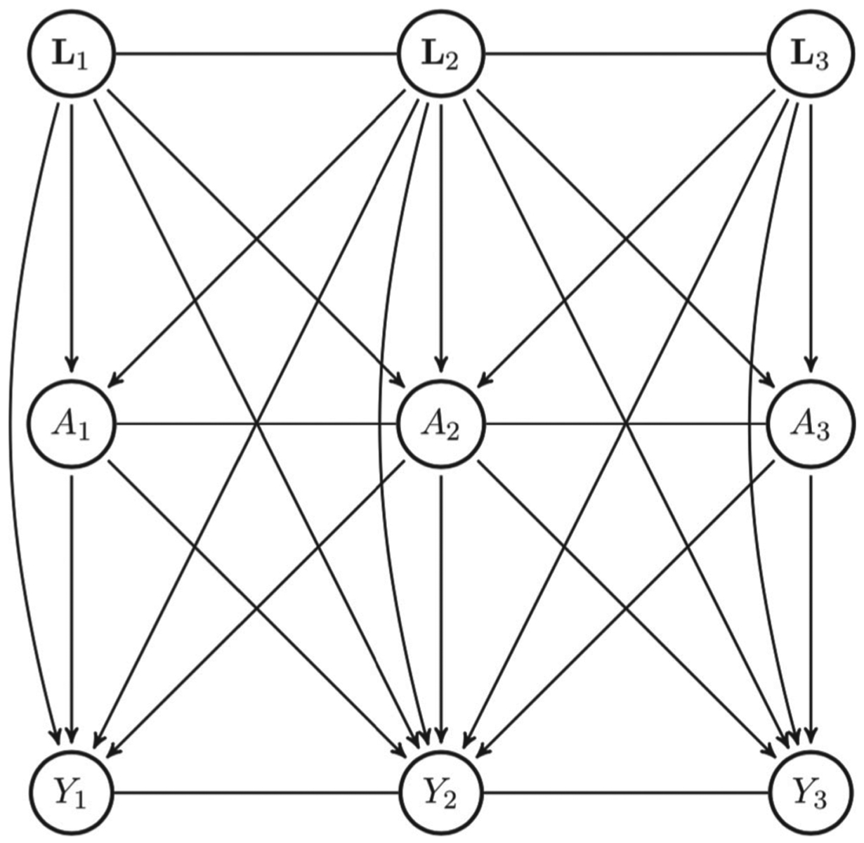
Chain graph representation of data from a network of three units.

We will assume the observed data distribution for O associated with our network causal model is Markov relative to the CG constructed from unit connections in a network via the above two level factorization (Lauritzen 1996). This implies the observed data distribution obeys certain conditional independence restrictions that one might intuitively expect to hold in a network, and which serve as the basis of the proposed approach. Let ${\mathcal{N}}_i$ denote the set of neighbors of unit i, that is, ${\mathcal{N}}_i=\left\{j:(i,j)\in \mathcal{E}\right\}$, and let ${\mathcal{O}}_i=\left\{{\text{O}}_j,j\in {\mathcal{N}}_i\right\}$ denote data observed on all neighbors of unit i. Given a CG ${\mathcal{G}}_{\mathcal{E}}$ with associated neighboring pairs $\mathcal{E}$, the following conditional independences follow by the global Markov property associated with CGs (Lauritzen 1996):

$$Y_i⫫\left\{Y_k,A_k,L_k\right\}\mid \left(A_i,L_i,{\mathcal{O}}_i\right)\text{ for all }i\text{ and }k,k\ne i;$$ (6)

$$L_i⫫L_{-i}\backslash {\mathcal{O}}_i\mid L_{-i}\cap {\mathcal{O}}_i\text{ for all }i\text{ and }k\notin {\mathcal{N}}_i,k\ne i.$$ (7)

In words, Equation (6) states that the outcome of a given unit can be screened-off (i.e., made independent) from the variables of all nonneighboring units by conditioning on the unit’s treatment and covariates as well as on all data observed on its neighboring units, where the neighborhood structure is determined by ${\mathcal{G}}_{\mathcal{E}}$. That is, $\left(A_i,L_i,{\mathcal{O}}_i\right)$ is the Markov blanket of Y_i in CG ${\mathcal{G}}_{\mathcal{E}}$. This assumption, coupled with a sparse network structure, leads to extensive dimension reduction of the model specification for Y|A, L. In particular, the conditional density of Y_i| {O\Y_i} only depends on (A_i, L_i) and on neighbors’ data ${\mathcal{O}}_i$. Similarly, $L_{-i}\cap {\mathcal{O}}_i$ is the Markov blanket of L_i in CG ${\mathcal{G}}_{\mathcal{E}}$.

3.2. Conditional Auto-models

Suppose that instead of (3), the following stronger positivity condition holds:

$$\mathbb{P}(O=o)>0,\text{ for all possible values }o.$$ (8)

Since (6) holds for the conditional law of Y given A, L, it lies in the conditional MRF (CMRF) model associated with the induced undirected graph ${\mathcal{G}}_{\mathcal{E}}^a$. In addition, since (8) holds, the conditional MRF version of the Hammersley–Clifford theorem and (6) imply the following version of the clique factorization in (5),

$$f(y\mid a,l)=\left(\frac{1}{\kappa (a,l)}\right)\text{ exp }\left\{U(y;a,l)\right\},$$

where $\kappa (a,l)={\sum }_{\text{y}}\text{exp }\left\{U(y;a,l)\right\}$, and U (y;a, l) is a conditional energy function which can be decomposed into a sum of terms called conditional clique potentials, with a term for every maximal clique in the graph ${\mathcal{G}}_{\mathcal{E}}^a$ (Besag 1974). Conditional clique potentials offer a natural way to specify a CMRF using only terms that depend on a small set of variables. Specifically,

$$\begin{gathered} f\left(Y_i=y_i\mid Y_{-i}=y_{-i},a,l\right) \\ =f\left(Y_i=y_i\mid Y_{-i}={\text{y}}_{-i},\left\{a_j,l_j:j\in {\mathcal{N}}_i\right\}\right) \\ =\frac{\text{exp }\left\{{\sum }_{c\in {\mathcal{C}}_i}{U}_c(y;a,l)\right\}}{{\sum }_{y^{\prime }:y_{-i}^{\prime }=y-i}\text{ exp }\left\{{\sum }_{c\in {\mathcal{C}}_i}{U}_c\left(y^{\prime };a,l\right)\right\}} \end{gathered}$$ (9)

where ${\mathcal{C}}_i$ are all maximal cliques of ${\mathcal{G}}_{\mathcal{E}}^a$ that involve Y_i.

Gibbs densities specified as in (9) is a rich class of densities, and are often regularized in practice by setting to zero conditional clique potentials for cliques of size greater than a prespecified cut-off. This type of regularization corresponds to setting higher order interactions terms to zero in log-linear models. For instance, closely following Besag (1974), one may introduce conditions (a) only cliques $c\in \mathcal{C}$ of size one or two have nonzero potential functions Uc, and (b) the conditional probabilities in (9) have an exponential family form. Under these additional conditions, given a, l, the energy function takes the form

$$U(y;a,l)=\sum _{i\in {\mathcal{G}}_{\mathcal{E}}}{y}_i{G}_i\left(y_i;a,l\right)+\sum _{\left\{i,j\right\}\in \mathcal{E}}{y}_i{y}_j{\theta }_{ij}(a,l),$$

for some functions G_i (·; a, l) and coefficients θ_ij (a, l). Note that to be consistent with local Markov conditions (6) and (7), G_i (·; a, l) can only depend on $\left\{\left(a_s,l_s\right):s\in {\mathcal{N}}_j\right\}$, on while because of symmetry θ_ij (a, l) can depend at most on $\left\{\left(a_s,l_s\right):s\in {\mathcal{N}}_j\cap {\mathcal{N}}_i\right\}$. Following Besag (1974), we call the resulting class of models conditional auto-models.

Conditions (7) and (8) imply that L is an MRF; standard Hammersley–Clifford theorem further implies that the joint density of L can be written as

$$f(l)=\left(\frac{1}{v}\right)\text{ exp }\left\{W(l)\right\},$$

where $v={\sum }_{l^{\prime }}\text{exp }\left\{W\left(l^{\prime }\right)\right\}$, and W (l) is an energy function which can be decomposed as a sum over cliques in the induced undirected graph ${(\mathcal{G}\mathcal{E})}_{\mathbf{\text{L}}}$. Analogous to the conditional auto-model described above, we restrict attention to densities of L of the form:

$$W(\mathbf{\text{L}})=\sum _{i\in {\mathcal{G}}_{\mathcal{E}}}\left\{\sum _{k=1}^p{L}_{k,i}{H}_{k,i}\left(L_{k,i}\right)+\sum _{k\ne s}{\rho }_{k,s,i}{L}_{k,i}{L}_{s,i}\right\}+\sum _{\left\{i,j\right\}\in \mathcal{E}}\sum _{k=1}^p\sum _{s=1}^p{\omega }_{k,s,i,j}{L}_{k,i}{L}_{s,j},$$ (10)

for some functions H_k,i (L_k,i) and coefficients ρ_k,s,i, ω_k,s,i,j. Note that ρ_k,s,i encodes the association between covariate L_k,i and covariate L_s,i observed on unit i, while ω_k,s,i,j captures the association between L_k,i observed on unit i and L_s,j observed on unit j.

3.3. Parametric Specifications of Auto-models

A prominent auto-regression model for binary outcomes is the so-called autologistic regression first proposed by Besag (1974). Note that as (a, l) is likely to be high dimensional, identification and inference about G_i and θ_ij requires one to further restrict heterogeneity by specifying simple low dimensional parametric models for these functions of the form:

$$\begin{gathered} G_i\left(y_i;a,l\right)={\tilde{G}}_i(a,l)=\text{log}\frac{\text{Pr }\left(Y_i=1\mid a,l,Y_{-i}=0\right)}{\text{Pr }\left(Y_i=0\mid a,l,Y_{-i}=0\right)} \\ ={\beta }_0+{\beta }_1{a}_i+{\beta }_2^{\prime }{l}_i+{\beta }_3\sum _{j\in {\mathcal{N}}_i}{w}_{ij}^a{a}_j+{\beta }_4^{\prime }\sum _{j\in {\mathcal{N}}_i}{w}_{ij}^l{l}_j; \\ {\theta }_{ij}=w_{ij}^y\theta , \end{gathered}$$

where $w_{ij}^a$, $w_{ij}^l$, $w_{ij}^y$ are user specified weights which may depend on network features associated with units i and j, with ${\sum }_j{w}_{ij}^a={\sum }_j{w}_{ij}^l={\sum }_j{w}_{ij}^y=1$ for example, $w_{ij}^a=1/\text{card }\left({\mathcal{N}}_i\right)$ standardizes the regression coefficient by the size of a unit’s neighbourhood. We assume model parameters $\tau =\left({\beta }_0,{\beta }_1,{\beta }_2^{\prime },{\beta }_3,{\beta }_4^{\prime },\theta \right)$ are shared across units in a network. In addition, network features can be incorporated into the auto-models as model parameters, which may be desirable in settings where network features are confounders for the relationship between exposure and outcome. For example, one could further adjust for a unit’s degree (i.e., number of ties).

For a continuous outcome, an auto-Gaussian model may be specified as followed:

$$\begin{gathered} G_i\left(y_i;a,l\right)=-\left(\frac{1}{2{\sigma }_y^2}\right)\left(y_i-2{\mu }_{y,i}(a,l)\right); \\ {\mu }_{y,i}(a,l)={\beta }_0+{\beta }_1{a}_i+{\beta }_2^{\prime }{l}_i+{\beta }_3\sum _{j\in {\mathcal{N}}_i}{w}_{ij}^a{a}_j+{\beta }_4^{\prime }\sum _{j\in {\mathcal{N}}_i}{w}_{ij}^l{l}_j; \\ {\theta }_{ij}=w_{ij}^y\theta , \end{gathered}$$

where μ_y,i (a, l) = E (Y_i|a, l, Y_−i = 0), and ${\sigma }_y^2=\text{var }\left(Y_i\mid a,l,Y_{-i}=0\right)$. Similarly, model parameters ${\tau }_Y=\left({\beta }_0,{\beta }_1,{\beta }_2^{\prime },{\beta }_3,{\beta }_4^{\prime },{\sigma }_y^2,\theta \right)$ are shared across units in the network. Other auto-models within the exponential family can likewise be conditionally specified, for example, the auto-Poisson model.

Auto-model density of L is specified similarly. For example, fix parameters in (10)

$${\rho }_{k,s,i}={\rho }_{k,s},$$

$${\omega }_{k,s,i,j}={\tilde{\omega }}_{k,s}{v}_{i,j},$$

where v_i,j is a user-specified weight which satisfies ${\sum }_j{v}_{i,j}=1.$. For L_k binary, one might take

$$H_{k,i}\left(L_{k,i};{\tau }_k\right)={\tau }_k=\text{log}\frac{\text{Pr }\left(L_{k,i}=1\mid L_{\backslash k,i}=0,L_{-i}=0\right)}{\text{Pr }\left(L_{k,i}=0\mid L_{\backslash k,i}=0,L_{-i}=0\right)},$$

corresponding to a logistic auto-model for L_k,i|L_\k,i 0, L_−i = 0, while for continuous L_k

$$H_{k,i}\left(L_{k,i};{\tau }_k=\left({\sigma }_k^2,{\mu }_k\right)\right)=-\left(\frac{1}{2{\sigma }_k^2}\right)\left(L_{k,i}-2{\mu }_k\right),$$

corresponding to a Gaussian auto-model for L_k,i|L_\k,i = 0, L_−i = 0. As before, model parameters ${\tau }_L=\left({\tau }_1^{\prime },\dots ,{\tau }_p^{\prime }\right)$ are shared across units in the network.

3.4. Coding Estimators of Auto-models

Suppose that one has specified auto-models for Y and L as in the previous section with unknown parameters τ_Y and τ_L, respectively. To estimate these parameters, one could in principle attempt to maximize the corresponding joint likelihood function. However, such task is well-known to be computationally daunting as it requires a normalization step which involves evaluating a high dimensional sum or integral which, outside relatively simple auto-Gaussian models is generally not available in closed form. For example, to evaluate the conditional likelihood of Y|A, L for binary Y requires evaluating a sum of 2^N terms to compute κ (A, L). Fortunately, less computationally intensive strategies for estimating auto-models exist including pseudo-likelihood (PL) estimation and so called-coding estimators (Besag 1974), which may be adopted here. We first consider coding-type estimators, mainly because unlike PL estimation, standard asymptotic theory applies. To describe these estimators in more detail requires additional definitions.

We define a stable set or independent set on ${\mathcal{G}}_{\mathcal{E}}$ as the set of nodes, $\mathcal{S}\left({\mathcal{G}}_{\mathcal{E}}\right)$, such that

$$(i,j)\notin \mathcal{E}\forall (i,j)\in \mathcal{S}\left({\mathcal{G}}_{\mathcal{E}}\right).$$

That is, a stable set is a set of nodes with the property that no two nodes in the set have an edge connecting them in the network. The size of a stable set is the number of units it contains. A maximal stable set is a stable set such that no unit in ${\mathcal{G}}_{\mathcal{E}}$ can be added without violating the independence condition. A maximum stable set ${\mathcal{S}}_{\text{max }}\left({\mathcal{G}}_{\mathcal{E}}\right)$ is a maximal stable set of largest possible size for ${\mathcal{G}}_{\mathcal{E}}$. This size is called the stable number or independence number of ${\mathcal{G}}_{\mathcal{E}}$, which we denote $n_{1,N}=n_1\left({\mathcal{G}}_{\mathcal{E}}\right)$ A maximum stable is not necessarily unique in a given graph, and finding one such set and enumerating them all is challenging but a well-studied problem of computer science. In fact, finding a maximum stable set is a well-known NP-complete problem. Nevertheless, both exact and approximate algorithms exist that are computationally more efficient than an exhaustive search. Exact algorithms which identify all maximum stable sets were described in Robson (1986), Makino and Uno (2004), and Fomin, Grandoni, and Kratsch (2009). Unfortunately, exact algorithms for finding maximum stable sets quickly become computationally prohibitive with moderate to large networks. In fact, the maximum stable set problem is known not to have an efficient approximation algorithm unless P = NP (Zuckerman 2006). A practical approach we take in this article is to simply use an enumeration algorithm that lists a collection of maximal stable sets (Myrvold and Fowler 2013), and pick the largest of the maximal sets found. Let ${\Xi }_1=\left\{{\mathcal{S}}_{\text{max }}\left({\mathcal{G}}_{\mathcal{E}}\right):\text{card }\left({\mathcal{S}}_{\text{max }}\left({\mathcal{G}}_{\mathcal{E}}\right)\right)={\text{n}}_1\left({\mathcal{G}}_{\mathcal{E}}\right)\right\}$ denote the collection of all maximum (or largest identified maximal) stable sets for ${\mathcal{G}}_{\mathcal{E}}$.

The Markov property associated with ${\mathcal{G}}_{\mathcal{E}}$ implies that outcomes of units within such sets are mutually conditionally independent given their Markov blankets. This implies the (partial) conditional likelihood function which only involves units in the stable set factorizes, suggesting that tools from maximum likelihood estimation may apply. In the Appendix, we establish that this is in fact the case, in the sense that under certain regularity conditions, coding maximum likelihood estimators of τ based on maximum (or largest identified maximal) stable sets are consistent and asymptotically normal (CAN). Consider the coding likelihood functions for τ_Y and τ_L based on a stable set ${\mathcal{S}}_{\text{max }}\left({\mathcal{G}}_{\mathcal{E}}\right)\in {\Xi }_1$:

$$\mathcal{C}{\mathcal{L}}_Y\left({\tau }_Y\right)=\prod _{i\in \mathcal{S}\text{max }\left({\mathcal{G}}_{\mathcal{E}}\right)}{\mathcal{L}}_{Y,{\mathcal{S}}_{\text{max }}\left({\mathcal{G}}_{\mathcal{E}}\right),i}\left({\tau }_Y\right)\#\#=\prod _{i\in {\mathcal{S}}_{\text{max }}\left({\mathcal{G}}_{\mathcal{E}}\right)}f\left(Y_i\mid {\mathcal{O}}_i,A_i,L_i;{\tau }_Y\right);$$ (11)

$$\begin{gathered} \mathcal{C}{\mathcal{L}}_L\left({\tau }_L\right)=\prod _{i\in {\mathcal{S}}_{\text{max }}\left({\mathcal{G}}_{\mathcal{E}}\right)}{\mathcal{L}}_{L,{\mathcal{S}}_{\text{max }}\left({\mathcal{G}}_{\mathcal{E}}\right),i}\left({\tau }_L\right) \\ =\prod _{i\in {\mathcal{S}}_{\text{max }}\left({\mathcal{G}}_{\mathcal{E}}\right)}f\left(L_i\mid \left\{L_j:j\in {\mathcal{N}}_i\right\};{\tau }_L\right). \end{gathered}$$ (12)

The estimators ${\widehat{\tau }}_Y=\text{arg }{\text{max }}_{{\tau }_Y}\text{log }\mathcal{C}{\mathcal{L}}_Y\left({\tau }_Y\right)$ and ${\widehat{\tau }}_L=\text{arg }{\text{max }}_{{\tau }_L}\text{log }\mathcal{C}{\mathcal{L}}_L\left({\tau }_L\right)$ are analogous to Besag’s coding maximum likelihood estimators. Consider a network asymptotic theory according to which $\left\{{\mathcal{G}}_{{\mathcal{E}}_N}:N\right\}$ is a sequence of chain graphs as N → ∞, with vertices $\left(A_{\mathcal{E}},L_{\mathcal{E}},Y_{\mathcal{E}}\right)$ that follow correctly specified auto-models with unknown parameters (τ_Y, τ_L), and with edges defined according to a sequence of networks ${\mathcal{E}}_N$ of increasing size. We establish the following result in the Appendix.

Result 1: Suppose that n_1,N → ∞ as N → ∞ then under conditions 1–6 given in the Appendix,

$${\widehat{\tau }}_L\underset{N\to \infty }{\to }\tau \text{in}\text{ probability };{\widehat{\tau }}_Y\underset{N\to \infty }{\to }\tau \text{in}\text{probability}.\sqrt{n_{1,N}}{\text{Γ}}_{n_{1,N}}^{1/2}\left(\widehat{{\tau }_L}-{\tau }_L\right)\underset{N\to \infty }{\to }N(0,I);\sqrt{n_{1,N}}{\text{Ω}}_{n_{1,N}}^{1/2}\left({\widehat{\tau }}_Y-{\tau }_Y\right)\underset{N\to \infty }{\to }N(0,I);{\text{Γ}}_{n_{1,N}}=\frac{1}{n_{1,N}}\sum _{i\in {\mathcal{S}}_{\text{max}}\left({\mathcal{G}}_{{\mathcal{E}}_N}\right)}{\left\{\frac{\partial \text{log}\mathcal{C}{\mathcal{L}}_{L,{\mathcal{S}}_{\text{max}}\left({\mathcal{G}}_{{\mathcal{E}}_N}\right),i}\left({\tau }_L\right)}{\partial {\tau }_L}\right\}}^{\otimes 2},{\text{Ω}}_{n_{1,N}}=\frac{1}{n_{1,N}}\sum _{i\in {\mathcal{S}}_{\text{max}}\left({\mathcal{G}}_{{\mathcal{E}}_N}\right)}{\left\{\frac{\partial \text{log}\mathcal{C}{\mathcal{L}}_{L,{\mathcal{S}}_{\text{max}}\left({\mathcal{G}}_{{\mathcal{E}}_N}\right),i}\left({\tau }_Y\right)}{\partial {\tau }_Y}\right\}}^{\otimes 2}.$$

Note that by the information equality, ${\Gamma }_{n_{1,N}}$ and ${\Omega }_{n_{1,N}}$ can be replaced by the standardized (by n_1,N) negative second derivative matrix of corresponding coding log-likelihood functions. Note also that condition n_1,N → ∞ as N → ∞ essentially rules out the presence of an ever-growing hub on the network as it expands with N, thus ensuring that there is no connected set of units in which majority of connections are concentrated asymptotically. Suppose that each unit on a network of size N is connected to no more than C_max < N, then according to Brooks’ Theorem, the stable number n_1,N satisfies the inequalities (Brooks 1941):

$$\frac{N}{C_{\text{max }}+1}\le n_{1,N}\le N.$$

This implies that in a network of bounded degree, n_1,N = O (N) is guaranteed to be of the same order as the size of the network; however n_1,N may grow at substantially slower rates (n_1,N = o(N)) if C_max is unbounded.

3.5. PL Estimation

Note that because L_i is likely multivariate, further computational simplification can be achieved by replacing $f\left(L_i\mid \left\{L_j:j\in {\mathcal{N}}_i\right\};{\tau }_L\right)$ with the PL function

$$\prod _{s=1}^{p}f\left(L_{s,i}\mid L_{\setminus s,i},\left\{L_j:j\in {\mathcal{N}}_i\right\};{\tau }_L\right)$$

in Equation (12). This substitution is computationally more efficient as it obviates the need to evaluate a multivariate integral to normalize the joint law of L_i. Let $\tilde{\tau }$ denote the estimator which maximizes the log of the resulting modified coding likelihood function ${\mathcal{L}}_{L,{\mathcal{S}}_{\text{max }}({\mathcal{G}}_{\mathcal{E}}),i}^{\ast }\left({\tau }_L\right)$. It is straightforward using the proof of Result 1 to establish that its covariance may be approximated by the sandwich formula ${\Phi }_{L,n_{1,N}}^{-1}{\Gamma }_{L,n_{1,N}}{\Phi }_{L,n_{1,N}}^{-1}$ (Guyon 1995), where

$$\begin{gathered} {\Gamma }_{L,n_{1,N}}=\frac{1}{n_{1,N}}\sum _{i\in {\mathcal{S}}_{\text{max }}\left({\mathcal{G}}_{\mathcal{E}}\right)}{\left\{\frac{\partial \text{ log }{\mathcal{L}}_{L,{\mathcal{S}}_{\text{max }}({\mathcal{G}}_{\mathcal{E}}),i}^{\ast }\left({\tau }_L\right)}{\partial {\tau }_L}\right\}}^{\otimes 2}, \\ {\Phi }_{L,n_{1,N}}=\frac{1}{n_{1,N}}\sum _{i\in {\mathcal{S}}_{\text{max }}\left({\mathcal{G}}_{\mathcal{E}}\right)}\left\{\frac{{\partial }^2\text{ log }{\mathcal{L}}_{L,{\mathcal{S}}_{\text{max }}(\mathcal{G}\epsilon ),i}^{\ast }\left({\tau }_L\right)}{\partial {\tau }_L\partial {\tau }_L^T}\right\}. \end{gathered}$$

As later illustrated in extensive simulation studies, coding estimators can be inefficient, since the partial conditional likelihood function associated with coding estimators disregards contributions of units $i\notin {\mathcal{S}}_{\text{max }}\left({\mathcal{G}}_{\mathcal{E}}\right)$. Substantial information may be recovered by combining multiple coding estimators each obtained from a separate approximate maximum stable set, however accounting for dependence between the different estimators can be challenging.

PL estimation offers a simple alternative approach which is potentially more efficient than either approach described above. PL estimators maximize the log-PLs

$$\text{log }\left\{\mathcal{P}{\mathcal{L}}_Y\left({\tau }_Y\right)\right\}=\sum _{i\in {\mathcal{G}}_{\mathcal{E}}}\text{log }f\left(Y_i\mid {\mathcal{O}}_i,A_i,L_i;{\tau }_Y\right);$$ (13)

$$\text{log }\left\{\mathcal{P}{\mathcal{L}}_L\left({\tau }_L\right)\right\}=\sum _{i\in {\mathcal{G}}_{\mathcal{E}}}\text{log }f(L_{k,i}\mid \left\{L_{s,i}:s\in \{1,\dots ,p\}\backslash k\right\},$$ (14)

$$\left\{L_{s,j}:s\in \{1,\dots ,p\},j\in {\mathcal{N}}_i\right\};{\tau }_L).$$ (15)

Denote corresponding estimators ${\check{\tau }}_{{}_Y}$ and ${\check{\tau }}_L$, which are shown to be consistent in the Appendix. There however is generally no guarantee that their asymptotic distribution follows a Gaussian distribution due to complex dependence between units on the network prohibiting application of the central limit theorem. As a consequence, for inference, we recommend using the parametric bootstrap, whereby algorithm Gibbs sampler I of Section 2.2 may be used to generate multiple bootstrap samples from the observed data likelihood evaluated at $\left({\check{\tau }}_{{}_Y},{\check{\tau }}_{{}_L}\right)$, which in turn can be used to obtain a bootstrap distribution for $\left({\check{\tau }}_{{}_Y},{\check{\tau }}_{{}_L}\right)$ and corresponding inferences such as bootstrap quantile confidence intervals.

4. Auto-G-Computation

We now return to the main goal of the article, which is to obtain valid inferences about β_i (a). The auto-G-computation algorithm entails evaluating

$${\widehat{\beta }}_i(a)\approx K^{-1}\sum _{k=0}^K{\widehat{Y}}_i^{\left(m^{\ast }+k\right)},$$

where ${\widehat{Y}}_i^{(m)}$ are generated by Gibbs Sampler I algorithm under posited auto-models with estimated parameters $\left({\widehat{\tau }}_Y,{\widehat{\tau }}_L\right)$. An analogous estimators ${\breve{\beta }}_i(\mathbf{a})$ can be obtained using $\left({\check{\tau }}_{{}_Y},{\check{\tau }}_{{}_L}\right)$ instead of $\left({\widehat{\tau }}_Y,{\widehat{\tau }}_L\right)$. In either case, the parametric bootstrap may be used in conjunction with Gibbs Sampler I to generate the corresponding bootstrap distribution of estimators of β_i (a) conditional on either ${\widehat{\beta }}_i(\mathbf{a})$ or ${\breve{\beta }}_i(\mathbf{a})$. Alternatively, a less computationally intensive approach first generates iid samples ${\tau }_Y^{(j)}$ and ${\tau }_L^{(j)},j=1,\dots ,J$ from $N\left({\widehat{\tau }}_Y,{\widehat{\Gamma }}_{n_{1,N}}\right)$ and $N\left({\widehat{\tau }}_L,{\widehat{\Omega }}_{n_{1,N}}\right)$, respectively, conditional on the data, where ${\widehat{\Gamma }}_{n_{1,N}}={\Gamma }_{n_{1,N}}\left(\widehat{{\tau }_L}\right)$ and ${\widehat{\Omega }}_{n_{1,N}}={\Omega }_{n_{1,N}}\left({\widehat{\tau }}_Y\right)$ estimate ${\Gamma }_{n_{1,N}}$ and ${\Omega }_{n_{1,N}}$. Next, one computes corresponding estimators ${\widehat{\beta }}_i^{(j)}(\mathbf{a})$ based on simulated data generated using Gibbs Sampler I algorithm under ${\tau }_Y^{(j)}$ and ${\tau }_L^{(j)},j=1,\dots ,J$. The empirical distribution of $\left\{{\widehat{\beta }}_i^{(j)}(\mathbf{a}):j\right\}$ may be used to obtain standard errors for ${\widehat{\beta }}_i(\mathbf{a})$, and corresponding Wald type or quantile-based confidence intervals for direct and spillover causal effects.

5. Simulation Study

We performed an extensive simulation study to evaluate the performance of the proposed methods on networks of varying density and size. Specifically, we investigated the properties of the coding-type and PL estimators of unknown parameters τ_Y and τ_L indexing the joint observed data likelihood. Additionally, we evaluated the performance of proposed estimators of the network counterfactual mean $\beta (\alpha )=N^{-1}{\sum }_{i=1}^N{\sum }_{a_{-i}\in \mathcal{A}(N)}{\pi }_i\left(a_{-i};\alpha \right)E\left(Y_i(a)\right)$, as well as for the direct effect DE(α), and the spillover effect IE(α), where α is a specified treatment allocation law described below.

We simulated three networks of size 800 with varying densities: low (each node has either 2, 3, or 4 neighbors), medium (each node has either 5, 6, or 7 neighbors), and high (each node has either 8, 9, or 10 neighbors). For reference, a depiction of the low density network of size 800 is given in Figure 2. Additionally, we simulated low density networks of size 200, 400, and 1000. The network graphs were all simulated in Wolfram Mathematica 10 using the RandomGraph function. For each network, we obtained an (approximate) maximum stable set. The stable sets for the 800 node networks were of size n_1,low = 375, n_1,med = 275, n_1,high = 224.

Figure 2.

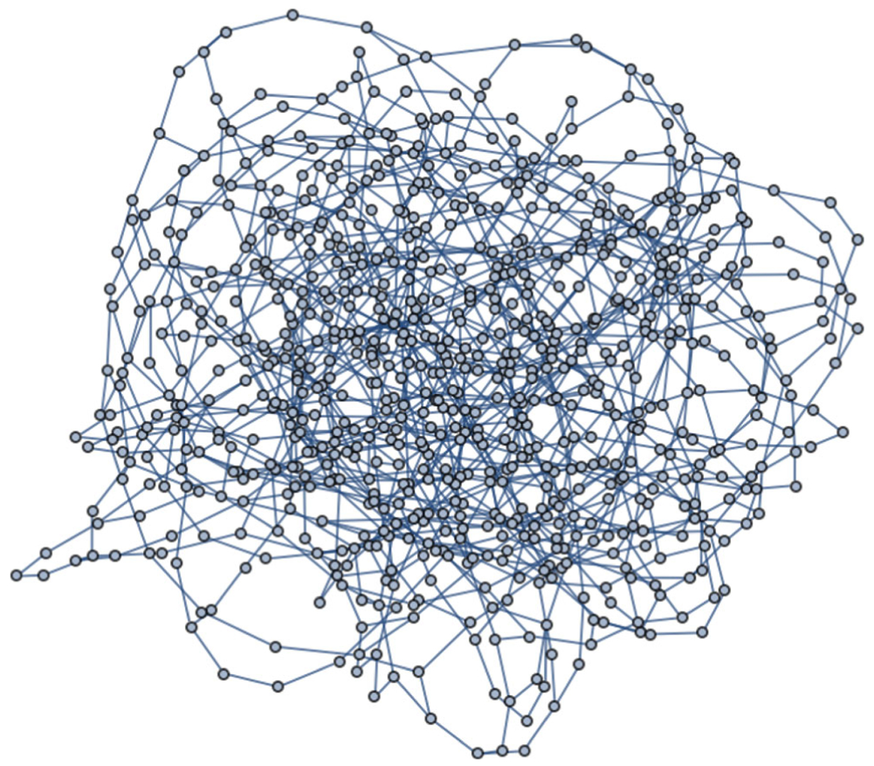
Network of size 800 with low density.

For units i = 1, … ,N, we generated using Gibbs Sampler I a vector of binary confounders {L_1i, L_2i, L_3i}, a binary treatment assignment A_i, and a binary outcome Y_i from the following auto-models consistent with the chain graph induced by the simulated network:

$$\begin{gathered} \text{Pr}\left(L_{1,i}=1\mid L_{\backslash 1,i},\left\{L_{1,j}:j\in {\mathcal{N}}_i\right\}\right) \\ =\text{expit}({\tau }_1+{\rho }_{12}{L}_{2,i}+{\rho }_{13}{L}_{3,i}+v_{11}\sum _{j\in {\mathcal{N}}_i}{L}_{1,j}+v_{12}\sum _{j\in {\mathcal{N}}_i}{L}_{2,j}+v_{13}\sum _{j\in {\mathcal{N}}_i}{L}_{3,j}), \end{gathered}$$

$$\begin{gathered} \text{Pr}\left(L_{2,i}=1\mid L_{\backslash 2,i},\left\{L_j:j\in {\mathcal{N}}_i\right\}\right) \\ =\text{expit}({\tau }_2+{\rho }_{12}{L}_{1,i}+{\rho }_{23}{L}_{3,i}+v_{21}\sum _{j\in {\mathcal{N}}_i}{L}_{1,j}+v_{22}\sum _{j\in {\mathcal{N}}_i}{L}_{2,j}+v_{23}\sum _{j\in {\mathcal{N}}_i}{L}_{3,j}), \end{gathered}$$

$$\begin{gathered} \text{Pr}\left(L_{3,i}=1\parallel L_{\backslash 3,i},\left\{L_j:j\in {\mathcal{N}}_i\right\}\right) \\ =\text{expit}({\tau }_3+{\rho }_{13}{L}_{1,i}+{\rho }_{23}{L}_{2,i}+v_{31}\sum _{j\in {\mathcal{N}}_i}{L}_{1,j}+v_{32}\sum _{j\in {\mathcal{N}}_i}{L}_{2,j}+v_{33}\sum _{j\in {\mathcal{N}}_i}{L}_{3,j}) \end{gathered}$$

$$\begin{gathered} \text{Pr}\left(A_i=1\mid L_i,\left\{A_j,{\text{L}}_j:j\in {\mathcal{N}}_i\right\}\right) \\ =\text{expit}({\gamma }_0+{\gamma }_1{L}_{1,i}+{\gamma }_2\sum _{j\in {\mathcal{N}}_i}{L}_{1,j}+{\gamma }_3{L}_{2,i}+{\gamma }_4\sum _{j\in {\mathcal{N}}_i}{L}_{2,j}+{\gamma }_5{L}_{3,i}+{\gamma }_6\sum _{j\in {\mathcal{N}}_i}{L}_{3,j}+{\gamma }_7\sum _{j\in {\mathcal{N}}_i}{A}_j) \end{gathered}$$

$$\begin{gathered} \text{Pr}\left(Y_i=1\mid A_i,L_i,{\mathcal{O}}_i\right) \\ =\text{expit}({\beta }_0+{\beta }_1{A}_i+{\beta }_2\sum _{j\in {\mathcal{N}}_i}{A}_j+{\beta }_3{L}_{1,i}+{\beta }_4\sum _{j\in {\mathcal{N}}_i}{L}_{1,j},+{\beta }_5{L}_{2,i}+{\beta }_6\sum _{j\in {\mathcal{N}}_i}{L}_{2,j}+{\beta }_7{L}_{3,i}+{\beta }_8\sum _{j\in {\mathcal{N}}_i}{L}_{3,j}+{\beta }_9\sum _{j\in {\mathcal{N}}_i}{Y}_j), \end{gathered}$$

where expit (x) = (1 + exp (−x))⁻¹, τ_L = {τ₁, τ₂, τ₃, ρ₁₂, ρ₁₃, ρ₂₃, ν₁₁, ν₁₂, ν₁₃, ν₂₂, ν₂₁, ν₂₃, ν₃₃, ν₃₁, ν₃₂}, = τ_A = {γ₀, … , γ₇}, and τ_Y = {β₀, … , β₉}. We evaluated network average direct and spillover effects via the Gibbs Sampler I algorithm under true parameter values τ_Y and τ_L and a treatment allocation, α given by a binomial distribution with event probability equal to 0.7. All parameter values are summarized in Table 1. We generated S = 1000 simulations of the chain graph for each of the 4 simulated network structures. For each simulation s, data were generated by running the Gibbs sampler I algorithm 4000 times with the first 1000 iterations as burn-in. Additionally, we thinned the chain by retaining every third realization to reduce autocorrelation.

Table 1.

True parameter values for simulation study.

Parameter	Truth
τL	(−1.0, 0.50, −0.50, 0.1, 0.2, 0.1, 0.1, 0, 0, 0.1, 0, 0, 0.1, 0, 0)
τA	(−1.00, 0.50, 0.10, 0.20, 0.05, 0.25, −0.08, 0.30)
τY	(−0.30, −0.60, −0.20, −0.20, −0.05, −0.10, −0.01, 0.40, 0.01, 0.20)

For each realization of the chain graph, ${\mathcal{G}}_{{\mathcal{E}}_N,s}$, we estimated τ_Y via coding-type maximum likelihood estimation and τ_L via the modified coding estimator. Both sets of parameters were also estimated via maximum PL estimation. For each estimator we computed corresponding causal effect estimators, their standard errors and 95% Wald confidence intervals as outlined in previous Sections estimation of auto-model parameters was performed in R using functions optim() and glm() (R Core Team 2013) network average causal effects were estimated using Gibbs Sampler I using the agcEffect function in the autognet R package by plugging in estimates for (τ_L, τ_Y) using K = 50 iterations and a burn-in of m* = 10 iterations. For variance estimation of the coding-type estimator, 200 bootstrap replications were used.

Simulation results for the various density networks of size 800 are summarized in Tables 2 and 3 for the following parameters: the network average counterfactual β(α), the network average direct effect, and the network average spillover effect. Both coding and PL estimators had small bias in estimating β(α) regardless of network density (absolute bias <0.01). Coverage of the coding estimator ranged between 93.1% and 94.5%. Biases were also small for both spillover and direct effects: the bias slightly increased with network density, but still stayed below an absolute bias of 0.01. Coverage of coding-based confidence intervals for direct effects ranged from 92.5% to 95.6%, while the coverage for spillover effects decreased slightly with network density from 93.7% to 92.2%. It is important to note that as the network structure changes with network size and density, the corresponding estimated parameters likewise vary and therefore it is not necessarily straightforward to compare performance of the methodology across network structure. Table 3 gives the MC variance for the PL estimator which confirms greater efficiency compared to the coding estimator given the significantly larger effective sample size used by PL. Appendix Tables 1–3 report bias and coverage for the network causal effect parameters for low density networks of size 200, 400, and 1000. Additionally, Appendix Figures 1 and 2 report bias and coverage for all 25 auto-model parameters in the low-density network of size 800. As predicted by theory, coding-type and PL estimators exhibit small bias. Additionally, coding-type estimators had approximately correct coverage, while PL estimators had coverage substantially lower than the nominal level for a number of auto-model parameters. These results confirm the anticipated failure of PL estimators to be asymptotically Gaussian. Most notably, the coverage for the outcome auto-model coefficient capturing dependence on neighbors’ outcomes β₉ was 81%, while coverage of the coding-type Wald CI for this coefficient was 94%. Although not shown here, the coverage results for the auto-model parameters are consistent across all simulations.

Table 2.

Simulation results of coding based estimators of network causal effects for networks of size 800 by density.

	Truth	Bias	MC variance	Robust variance	95% CI coverage
Low (n1 = 375)
β(α)	0.211	0.001	0.001	0.001	0.945
Spillover	−0.166	0.002	0.004	0.004	0.937
Direct	−0.179	0.002	0.002	0.002	0.943
Medium (n1 = 275)
β(α)	0.209	0.003	0.001	0.002	0.931
Spillover	−0.170	0.007	0.013	0.015	0.925
Direct	−0.178	<0.001	0.003	0.003	0.925
High (n1 = 224)
β(α)	0.208	0.004	0.005	0.004	0.937
Spillover	−0.171	0.001	0.032	0.027	0.922
Direct	−0.177	−0.001	0.004	0.004	0.956

Table 3.

Simulation results of pseudo-likelihood based estimators of network causal effects for networks of size 800 by density. Confidence intervals for PL estimators were not calculated as they were shown to have invalid coverage in simulation studies.

	Truth	Absolute bias	MC variance
Low
β(α)	0.211	0.001	< 0.001
Spillover	−0.166	0.002	0.002
Direct	−0.179	0.002	0.001
Medium
β(α)	0.209	0.003	0.001
Spillover	−0.170	0.007	0.005
Direct	−0.178	<0.001	0.001
High
β(α)	0.208	0.004	0.001
Spillover	−0.171	0.001	0.006
Direct	−0.177	−0.001	0.001

We also assessed the performance of auto-g-computation in small, dense networks and in the presence of missing network edges. For the first, we generated one network of size 100 (n_1,100 = 25) and an additional network of size 200 (n_1,200 = 57). For the network of size 100, coding estimation of auto-model parameters in 437 of the 1000 simulated samples had convergence issues due to the small size of the maximal independent set. Excluding results with convergence issues, the causal estimates were biased and did not have correct coverage (see Appendix Figure 3(a)). The performance for the network of size 200 was much improved across these endpoints, though oftentimes the confidence intervals were too wide to be informative. In both cases, the PL estimator exhibited less bias than the coding estimator. In the previously described dense network of size 800, we randomly removed 564 (14%) of edges. The estimated parameters from the auto-models were unbiased and had correct coverage (see Appendix Figure 4). However, the causal estimates for both the coding and PL estimators exhibited bias, and the coding estimator had coverage slightly below the nominal level with the estimated spillover effect shifted toward null (see Appendix Figure 5).

6. Data Application

We consider an application of the auto-g-computation algorithm to the Networks, Norms, and HIV/STI Risk Among Youth (NNAHRAY) study to assess the effect of past incarceration on infection with HIV, STI, or Hepatitis C accounting for the network structure (Khan et al. 2009). The NNAHRAY study was conducted in a New York neighborhood with epidemic HIV and widespread drug use from 2002 to 2005 (Friedman et al. 2008). Through in-person interviews, information was collected regarding the respondents’ demographic characteristics, incarceration history, sexual partnerships and histories, and past drug use. At the time of the interviews, respondents were also tested for HIV, gonorrhea, chlamydia, herpes simplex virus (HSV) 2, hepatitis C virus (HCV), and syphilis. The study population we consider includes all interviewed persons with recorded results from their HIV, STI, and HCV tests (n = 8 persons missing) for a total sample size of N = 457 persons. We assume that HIV/STI/HCV status is missing completely at random. We defined a network tie (i.e., edge) as a sexual and/or injection drug use partnership in the past three months if at least one of the partners reported the relationship. The network structure is given in Figure 3. The number of partners (i.e., neighbors) for each respondent varied from none to 10 resulting in a maximal independent set of n₁ = 274.

Figure 3.

Network graph from the NNAHRAY data (N = 457) with individuals in the maximal independent set (n₁ = 274) in blue.

We estimated the network-level spillover and direct effect of past incarceration on infection with HIV, STI, or HCV under a Bernoulli allocation strategy with treatment probability equal to 0.50. Past incarceration was defined as any amount of jail time in the respondents’ history. We accounted for confounding by Latino/a ethnicity, age, education, and past illicit drug use. The same models and estimation procedure detailed in the simulation section were utilized; note that ν_ij where i ≠ j were assumed to be 0. For comparison, the auto-model parameters were estimated using the coding-type and PL estimators. Network average spillover and direct effects were restricted to persons with at least one network tie.

Table 4 gives the outcome auto-model parameter point estimates for the coding and PL estimators with 95% confidence intervals for the coding estimators excluding the covariate terms. Due to scaling by number of network ties, the outcome and exposure influence of network ties can be interpreted as the effect of average covariate value among network ties. Individuals who experienced prior incarceration had 2.12 [95% CI: 1.07–4.21] times the odds of infection with HIV/STI/HCV compared to those without prior incarceration. However, the incarceration status of network ties was not significantly associated with a person’s risk of HIV/STI/HCV (OR = 1.21 [95% CI: 0.52–2.84]) conditional on the neighbors’ outcomes. Individual’s with a greater proportion of their ties infected with HIV, STI, and/or HCV were much more likely to be infected with HIV, STI, and/or HCV (OR = 3.07 [95% CI: 1.33–7.09]). The PL point estimates were similar to the coding results. The full results for auto-model parameters from both the covariate and outcome model are given in Appendix Figure 6. The network average direct effect is 0.14 [95% CI: 0.02–0.28] when the proportion of persons with prior history of incarceration is 0.50. There was no significant evidence of a spillover effect of incarceration on HIV/STI/HCV risk over the network, as increasing the proportion of persons with a history of incarceration from 0 to 0.50 resulted in a negligible increase in average HIV/STI/HCV risk of a person with no prior incarceration [$\widehat{\text{DE}}=0.04$; 95% CI: −0.06 to 0.14].

Table 4.

Outcome auto-model parameters estimates for coding and pseudo-likelihood estimators (excluding covariates) on the odds ratio scale. Confidence intervals for PL estimators were not calculated as they were shown to have invalid coverage in simulation studies.

	Estimates	95% CI
Coding
Past incarceration status (individual)	2.12	[1.07, 4.21]
Past incarceration status (neighbors)	1.21	[0.52, 2.84]
HIV/STI/HCV status (neighbors)	3.07	[1.33, 7.09]
Pseudo-likelihood
Past incarceration status (individual)	2.36	–
Past incarceration status (neighbors)	0.97	–
HIV/STI/HCV status (neighbors)	2.62	–

In the Appendix, we have included two alternate outcome auto-model specifications that incorporate the number of sexual and injection drug use partners for each person in the network. In an infection disease setting, the number of partners should in principle be accounted for in the analysis as it is likely a confounder for the effect of incarceration (both individual and neighbors’ status) on infection status (Khan et al. 2018). As shown in the Appendix, adjusting for the number of network ties (e.g., sexual and injection drug partners) did not change our conclusions. Lastly, we performed two simulation studies based on the NNAHRAY network under the sharp null. Results are provided in the Appendix Tables 7 and 8.

7. Conclusion

We have described a new approach for evaluating causal effects on a network of connected units. Our methodology relies on the crucial assumption that accurate information on network ties between observed units is available to the analyst, which may not always be the case in practice. In fact, as demonstrated in our simulation study, bias may ensue if information about the network is incomplete, and therefore one fails to account for all existing ties. In future work, we plan to further develop our methods to appropriately account for uncertainty about the underlying network structure.

Another limitation of the proposed approach is that it relies heavily on parametric assumptions and as a result may be open to bias due to model misspecification. Although this limitation also applies to standard g-computation for iid settings which nevertheless has gained prominence in epidemiology (Robins, Hernán, and Siebert 2004; Taubman et al. 2009; Daniel, De Stavola, and Cousens 2011), our parametric auto-models which are inherently non-iid may be substantially more complex, as they must appropriately account both for outcome and covariate dependence, as well as for interference. Developing appropriate goodness-of-fit tests for auto-models is clearly a priority for future research. In addition, to further alleviate concerns about modeling bias, we plan in future work to extend semiparametric models such as structural nested models to the network context. Such developments may offer a real opportunity for more robust inference about network causal effects.

References

- Aronow PM (2012), “A General Method for Detecting Interference Between Units in Randomized Experiments,” Sociological Methods & Research, 41, 3–16. [Google Scholar]
- Aronow PM, and Samii C (2017), “Estimating Average Causal Effects Under General Interference, With Application to a Social Network Experiment,” The Annals of Applied Statistics, 11, 1912–1947. [Google Scholar]
- Athey S, Eckles D, and Imbens GW (2018), “Exact p-Values for Network Interference,” Journal of the American Statistical Association, 113, 230–240. [Google Scholar]
- Besag J (1974), “Spatial Interaction and the Statistical Analysis of Lattice Systems,” Journal of the Royal Statistical Society, Series B, 36, 192–225. [Google Scholar]
- Bowers J, Fredrickson MM, and Panagopoulos C (2013), “Reasoning About Interference Between Units: A General Framework,” Political Analysis, 21, 97–124. [Google Scholar]
- Brooks RL (1941), “On Colouring the Nodes of a Network,” in Mathematical Proceedings of the Cambridge Philosophical Society (Vol. 37), Cambridge University Press, pp. 194–197. [Google Scholar]
- Cox DR (1958), Planning of Experiments, New York: Wiley. [1,3] [Google Scholar]
- Daniel RM, De Stavola BL, and Cousens SN (2011), “gformula: Estimating Causal Effects in the Presence of Time-Varying Confounding or Mediation Using the g-Computation Formula,” Stata Journal, 11, 479. [Google Scholar]
- Ferracci M, Jolivet G, and van den Berg GJ (2014), “Evidence of Treatment Spillovers Within Markets,” Review of Economics and Statistics, 96, 812–823. [Google Scholar]
- Fomin FV, Grandoni F, and Kratsch D (2009), “A Measure & Conquer Approach for the Analysis of Exact Algorithms,” Journal of the ACM, 56, 25. [Google Scholar]
- Friedman S, Bolyard M, Sandoval M, Mateu-Gelabert P, Maslow C, and Zenilman J (2008), “Relative Prevalence of Different Sexually Transmitted Infections in HIV-Discordant Sexual Partnerships: Data From a Risk Network Study in a High-Risk New York Neighbourhood,” Sexually Transmitted Infections, 84, 17–18. [DOI] [PubMed] [Google Scholar]
- Graham BS (2008), “Identifying Social Interactions Through Conditional Variance Restrictions,” Econometrica, 76, 643–660. [Google Scholar]
- Guyon X (1995), Random Fields on a Network: Modeling, Statistics, and Applications, New York: Springer. [Google Scholar]
- Halloran ME, and Hudgens MG (2016), “Dependent happenings: a recent Methodological Review,” Current Epidemiology Reports, 3, 297–305. [DOI] [PMC free article] [PubMed] [Google Scholar]
- Hammersley JM, and Clifford P (1971), “Markov Fields on Finite Graphs and Lattices,” unpublished manuscript, 46. [Google Scholar]
- Hong G, and Raudenbush SW (2006), “Evaluating Kindergarten Retention Policy: A Case Study of Causal Inference for Multilevel Observational Data,” Journal of the American Statistical Association, 101, 901–910. [Google Scholar]
- Hudgens MG, and Halloran ME (2008), “Toward Causal Inference With Interference,” Journal of the American Statistical Association, 103, 832–842. [DOI] [PMC free article] [PubMed] [Google Scholar]
- Khan MR, Doherty IA, Schoenbach VJ, Taylor EM, Epperson MW, and Adimora AA (2009), “Incarceration and High-Risk Sex Partnerships Among Men in the United States,” Journal of Urban Health, 86, 584–601. [DOI] [PMC free article] [PubMed] [Google Scholar]
- Khan MR, Scheidell JD, Golin CE, Friedman SR, Adimora AA, Lejuez CW, Hu H, Quinn K, and Wohl DA (2018), “Dissolution of Committed Partnerships During Incarceration and STI/HIV-Related Sexual Risk Behavior After Prison Release Among African American Men,” Journal of Urban Health, 95, 479–487. [DOI] [PMC free article] [PubMed] [Google Scholar]
- Kolaczyk ED, and Csárdi G (2014), Statistical Analysis of Network Data With R (Vol. 65), New York: Springer. [Google Scholar]
- Lauritzen SL (1996), Graphical Models (Vol. 17), Oxford: Clarendon Press. [Google Scholar]
- Lauritzen SL, and Richardson TS (2002), “Chain Graph Models and Their Causal Interpretations,” Journal of the Royal Statistical Society, Series B, 64, 321–348. [Google Scholar]
- Liu JS (2008), Monte Carlo Strategies in Scientific Computing, New York: Springer. [Google Scholar]
- Liu L, and Hudgens MG (2014), “Large Sample Randomization Inference of Causal Effects in the Presence of Interference,” Journal of the American Statistical Association, 109, 288–301. [DOI] [PMC free article] [PubMed] [Google Scholar]
- Liu L, Hudgens MG, and Becker-Dreps S (2016), “On Inverse Probability-Weighted Estimators in the Presence of Interference,” Biometrika, 103, 829–842. [DOI] [PMC free article] [PubMed] [Google Scholar]
- Lundin M, and Karlsson M (2014), “Estimation of Causal Effects in Observational Studies With Interference Between Units,” Statistical Methods & Applications, 23, 417–433. [Google Scholar]
- Makino K, and Uno T (2004), “New Algorithms for Enumerating All Maximal Cliques,” in Scandinavian Workshop on Algorithm Theory, Springer, pp. 260–272. [Google Scholar]
- Manski CF (2013), “Identification of Treatment Response With Social Interactions,” The Econometrics Journal, 16, S1–S23. [Google Scholar]
- Myrvold W, and Fowler P (2013), “Fast Enumeration of All Independent Sets Up to Isomorphism,” Preprint. [Google Scholar]
- Ogburn EL, Sofrygin O, Diaz I, and van der Laan MJ (2017), “Causal Inference for Social Network Data,” arXiv no. 1705.08527. [DOI] [PMC free article] [PubMed] [Google Scholar]
- Ogburn EL, and VanderWeele TJ (2014), “Causal Diagrams for Interference,” Statistical Science, 29, 559–578. [Google Scholar]
- Pearl J (2000), Causality: Models, Reasoning and Inference (Vol. 29), New York: Springer. [Google Scholar]
- Richardson TS, and Robins JM (2013), “Single World Intervention Graphs (SWIGS): A Unification of the Counterfactual and Graphical Approaches to Causality,” Center for the Statistics and the Social Sciences, University of Washington Series, Working Paper, 128. [Google Scholar]
- Robins JM (1986), “A New Approach to Causal Inference in Mortality Studies With a Sustained Exposure Period Application to Control of the Healthy Worker Survivor Effect,” Mathematical Modelling, 7, 1393–1512. [Google Scholar]
- Robins JM, Hernán MA, and Siebert U (2004), “Effects of Multiple Interventions,” in Comparative Quantification of Health Risks: Global and Regional Burden of Disease Attributable to Selected Major Risk Factors (Vol. 1), eds. Ezzati M, Lopez AD, Rodgers A and Murray CJL, Geneva: World Health Organization, pp. 2191–2230. [Google Scholar]
- Robson JM (1986), “Algorithms for Maximum Independent Sets,” Journal of Algorithms, 7, 425–440. [Google Scholar]
- Rosenbaum PR (2007), “Interference Between Units in Randomized Experiments,” Journal of the American Statistical Association, 102, 191–200. [DOI] [PMC free article] [PubMed] [Google Scholar]
- Rubin DB (1974), “Estimating Causal Effects of Treatments in Randomized and Nonrandomized Studies,” Journal of Educational Psychology, 66, 688. [Google Scholar]
- Shpitser I, Tchetgen Tchetgen E, and Andrews R (2017), “Modeling Interference via Symmetric Treatment Decomposition,” arXiv no. 1709.01050. [Google Scholar]
- Sobel ME (2006), “What Do Randomized Studies of Housing Mobility Demonstrate? Causal Inference in the Face of Interference,” Journal of the American Statistical Association, 101, 1398–1407. [Google Scholar]
- Sofrygin O, and van der Laan MJ (2017), “Semi-Parametric Estimation and Inference for the Mean Outcome of the Single Time-Point Intervention in a Causally Connected Population,” Journal of Causal Inference, 5, 1–35. [DOI] [PMC free article] [PubMed] [Google Scholar]
- Taubman SL, Robins JM, Mittleman MA, and Hernán MA (2009), “Intervening on Risk Factors for Coronary Heart Disease: An Application of the Parametric g-Formula,” International Journal of Epidemiology, 38, 1599–1611. [DOI] [PMC free article] [PubMed] [Google Scholar]
- Tchetgen Tchetgen EJ, and VanderWeele TJ (2012), “On Causal Inference in the Presence of Interference,” Statistical Methods in Medical Research, 21, 55–75. [DOI] [PMC free article] [PubMed] [Google Scholar]
- VanderWeele TJ, Tchetgen Tchetgen EJ, and Halloran ME (2012), “Components of the Indirect Effect in Vaccine Trials: Identification of Contagion and Infectiousness Effects,” Epidemiology, 23, 751. [DOI] [PMC free article] [PubMed] [Google Scholar]
- Tchetgen Tchetgen EJ, and VanderWeele TJ (2014), “Interference and Sensitivity Analysis,” Statistical Science: A Review Journal of the Institute of Mathematical Statistics, 29, 687. [DOI] [PMC free article] [PubMed] [Google Scholar]
- Verbitsky-Savitz N, and Raudenbush SW (2012), “Causal Inference Under Interference in Spatial Settings: A Case Study Evaluating Community Policing Program in Chicago,” Epidemiologic Methods, 1, 107–130. [Google Scholar]
- Westreich D, Cole SR, Young JG, Palella F, Tien PC, Kingsley L, Gange SJ, and Hernán MA (2012), “The Parametric g-Formula to Estimate the Effect of Highly Active Antiretroviral Therapy on Incident Aids or Death,” Statistics in Medicine, 31, 2000–2009. [DOI] [PMC free article] [PubMed] [Google Scholar]
- Zuckerman D (2006), “Linear Degree Extractors and the Inapproximability of Max Clique and Chromatic Number,” in Proceedings of the Thirty-Eighth Annual ACM Symposium on Theory of Computing, ACM, pp. 681–690. [Google Scholar]
Associated Data
This section collects any data citations, data availability statements, or supplementary materials included in this article.