

Proteomic allocation modeling coupled with metaproteomics reveals that cellular costs govern micronutrient-controlled growth.
Abstract
Micronutrients control phytoplankton growth in the ocean, influencing carbon export and fisheries. It is currently unclear how micronutrient scarcity affects cellular processes and how interdependence across micronutrients arises. We show that proximate causes of micronutrient growth limitation and interdependence are governed by cumulative cellular costs of acquiring and using micronutrients. Using a mechanistic proteomic allocation model of a polar diatom focused on iron and manganese, we demonstrate how cellular processes fundamentally underpin micronutrient limitation, and how they interact and compensate for each other to shape cellular elemental stoichiometry and resource interdependence. We coupled our model with metaproteomic and environmental data, yielding an approach for estimating biogeochemical metrics, including taxon-specific growth rates. Our results show that cumulative cellular costs govern how environmental conditions modify phytoplankton growth.
INTRODUCTION
Marine phytoplankton are responsible for approximately half of global net primary productivity, supporting key ecosystem services (1). Micronutrients, such as iron, are often depleted in the ocean, limiting phytoplankton growth and therefore affecting fisheries productivity and carbon export globally (2–4). These resources are cofactors for enzymes that catalyze intracellular reactions, and unlike the macronutrients nitrogen and phosphorus, they comprise a negligible fraction of biomass. Cellular micronutrient stoichiometry is highly variable (5), and elements can conditionally substitute for one another (6). Therefore, traditional approaches that simply link growth rate to resource scarcity may not apply.
Growth is the emergent outcome of a range of internal cellular processes competing for shared resources (7) that are governed by costs [e.g., number of amino acids per protein or energetic requirements (8–10)] and constraints [e.g., limits of protein density in a membrane (11)]. Protein synthesis capacity has been identified as a key growth-limiting process in model heterotrophic organisms with various carbon sources (12, 13). Only recently have other noncarbon macronutrients been considered and additional complexities been revealed (14) [e.g., transcriptional limitation under low phosphorus (7)]. Currently, we lack knowledge regarding which internal processes limit growth under micronutrient deficiency. Furthermore, while we know that multiple nutrients can simultaneously affect growth rate (15), the mechanisms by which they interact appear to vary for each nutrient pair (6).
The overriding conceptual view in oceanography is not sufficient to mechanistically represent micronutrient limitation and resource interdependence. Currently, external resource scarcity (e.g., bioavailable forms of nitrogen, phosphorus, iron, etc.), relative to fixed requirements, is assumed to control growth and carbon fixation rates (16, 17). However, this ignores the role of internal processes in limiting growth. It also prevents general mechanisms of resource interdependence, which may arise because different internal processes compete for shared cellular resources from being included in large-scale ocean models. While external resource scarcity is clearly the ultimate cause of limitation, the proximate causes drive the sensitivity to environmental change. For example, temperature-driven changes in ribosomal translation rates might influence cellular nitrogen-to-phosphorus ratios because ribosomes are a large portion of phosphorus quotas (18). Currently, ocean models used for climate change projections parameterize growth as a simple function of the single most limiting resource (17), which introduces substantial uncertainties in a changing environment (3). While some phytoplankton models have leveraged quantitative, mechanistic insights into cellular processes (18–23), none have examined interactions between micronutrients or used in situ gene expression data to resolve cellular processes.
In this study, we quantify the proximate costs and constraints associated with micronutrient limitation via a novel coupling of cellular modeling and metaproteomics from the Southern Ocean. By deriving a phenomenological model, we identify key factors controlling interdependence across micronutrients. Last, we demonstrate a framework for inferring critical biogeochemical metrics, such as growth rates, by coupling in situ gene expression and geochemical data with cellular modeling. Together, this framework quantifies cellular costs and constraints to examine the mechanistic underpinnings of phytoplankton growth in the ocean.
RESULTS AND DISCUSSION
Estimating cellular costs and constraints with a diatom proteomic allocation model
We estimated the cellular costs and constraints of micronutrient limitation in phytoplankton by developing a mechanistic, proteomic allocation model for the polar diatom Fragilariopsis cylindrus (24, 25). Our model considers the essential micronutrients iron and manganese, which both influence primary productivity in the Southern Ocean (4, 26–28), and represents the various processes underlying cellular growth, such as photosynthesis and translation (25, 29–31). The model is composed of several “coarse-grained” protein pools (i.e., proteins grouped together with related functions; Fig. 1A): iron- and manganese-specific transporters, photosystem units, nitrogen uptake and metabolism (from nitrate to amino acids), and antioxidants [represented here by manganese superoxide dismutase (MnSOD)]. Each protein pool has an associated cost, which is proportional to the number of amino acids per pool [estimated using the F. cylindrus genome (24)]. Ribosomes are assumed to be allocated to maximize the steady-state specific growth rate, and each protein pool, metabolite, and internal free pool of Fe and Mn is described by an ordinary differential equation (ODE). The system of ODEs is connected by various stoichiometric coefficients obtained from the literature, for example, Mn atoms per MnSOD or the total number of Fe atoms within all proteins involved in converting nitrate into amino acids. We then integrated the system of ODEs forward in time to obtain steady-state estimates of each state variable, from which we calculate the specific growth rate. In our model, we define the specific growth rate as the rate of biosynthesis of amino acids relative to the average protein per cell (25). We used Bayesian optimization to determine the optimal ribosomal allocation under a given set of dissolved Mn (dMn), Fe (dFe), and light conditions (Materials and Methods). Iron and Mn interact via oxidative stress, where under low dFe, electrons leak more frequently from electron transport (32), thus increasing the requirement for the Mn-containing antioxidant SOD (33). Under low antioxidant availability, the cell must replace proteins damaged by reactive oxygen species (ROS) by increasing protein synthesis. Accordingly, the mismatch between superoxide production and its consumption via MnSOD leads to a protein synthesis rate penalty in our model (see Materials and Methods).
Fig. 1. A polar diatom-based proteomic allocation model combined with metaproteomic observations reproduces expected cell behavior.

(A) Schematic of proteomic allocation model. Micronutrients are taken up via nutrient-specific protein transporters (left). Internal pools of Mn and Fe (black boxes) are then accessible for protein synthesis. Photosystems require both Fe and Mn and are the source of energetic equivalents (“e”; black box), which are then used by protein synthesis, micronutrient uptake, and nitrogen metabolism (the latter two are not shown with arrows). Protein pools are synthesized via ribosomes and represented with circle-ended lines. All model runs were conducted with nitrate at saturating levels. (B) Growth rates across a range of Fe and Mn concentrations are quantitatively similar to growth rates in culture (fig. S4). (C) Fe transporters decrease with increased Fe concentrations (dMn = 500 pM), a commonly observed phenomena in cultures (49, 70).
We then leveraged proteomic and metaproteomic data to estimate three key costs and constraints: (i) internal Fe and Mn protein cost, (ii) available membrane space for transporters (34), and (iii) catalytic efficiency of MnSOD (Materials and Methods). (i) refers to all proteins required for acquiring, shuttling, and storing Fe within the cell [e.g., ferritin (35)], which is dynamic such that Fe protein cost increases with Fe quota (an identical cost is applied for Mn; see Supplementary Discussion). (ii) refers to the proportion of membrane space available for metal transporters (11, 34), for which we extended a mechanistic nutrient uptake model (36–38), accounting for competition for membrane space between iron and manganese transporters. (iii) represents the effectiveness of a single MnSOD unit.
Model parameters were estimated using Approximate Bayesian Computation (ABC) in a novel combination with diatom proteomes inferred from a metaproteomic time series (39). The metaproteome characterization coupled peptide mass spectrometry with metatranscriptomics (40) to examine protein expression over time at the Antarctic sea ice edge, where concurrent bottle incubations indicated a transition into micronutrient stress [cobalamin, Mn, and Fe (28, 41)]. Coarse-grained diatom protein pool biomass was estimated using the sum of diatom-specific peptide intensities (fig. S1) (42). Coarse-graining is necessary to prevent biases in peptide detectability and quantification across complex samples (43). Last, we combined the inferred diatom proteome observations with two previously published diatom proteomic datasets to estimate each parameter (Materials and Methods; fig. S2) (44, 45). We have assessed various forms of biases and developed methods for connecting environmental gene expression data to quantitative models of cellular processes (Materials and Methods), providing a path forward to leverage large-scale datasets in this way.
Our model reproduces expected cellular behavior across a range of dFe and dMn concentrations (Fig. 1, B and C, and fig. S3; using posterior modes for estimated parameters, fig. S2). For example, the model quantitatively reproduces growth rates (46), Mn and Fe cellular quotas (33, 47), and dFe uptake rates within observational constraints (48), despite no prescribed parameterization or model training on these data types (figs. S4 to S7). We are also able to reproduce the observed increase in transporters under low dFe and dMn (Fig. 1C and fig. S8) (20, 49), the expected interaction between light and Fe quota (fig. S9 and Supplementary Discussion) (50), and the increase in ribosomes with growth rate (Fig. 2 and fig. S8) (13, 51). Our analysis suggests that dMn and dFe interactively influence growth more at high dFe, rather than at low dFe, and a reframing of previous results supports this conclusion (fig. S10, Supplementary Discussion). Overall, these results show that our model is able to represent how diatom cells respond in different environments and is consistent with a variety of empirical observations.
Fig. 2. Cellular costs and constraints influence growth rate across a range of Fe and Mn concentrations.

(A) Model experiments showing how a fivefold increase in each parameter value influences growth rate, relative to the base model. Note that the parameter Fixed Proteome Percentage is divided by 5. (B) Micronutrient-controlled growth is the outcome of a range of internal processes, simultaneously controlling growth rate (proximate processes controlling growth rate are shown with black arrows). These internal processes are a function of cellular costs and constraints. (C) One internal, modeled process directly controlling growth is the number of ribosomes per cell, shown across iron and manganese concentrations.
Multiple internal processes, governed by cellular costs and constraints, control growth
Internal processes, which are a function of cellular costs, are the proximate causes of limitation. We conducted a set of computational experiments by systematically increasing each model parameter, which allowed us to examine the effect of different internal processes on growth (Fig. 2A and figs. S11 and S12). As expected, increasing stoichiometric coefficients for micronutrients (e.g., Fe per photosystem unit) had large, negative impacts on growth rates (Fig. 2A). However, protein costs (in terms of amino acids), internal rates, and energetic costs also had similarly large impacts (Fig. 2A). Moreover, the magnitude by which a given process affected growth differed depending on both dMn and dFe concentrations, illustrating the inadequacy of a simple “single-resource scarcity” view that underpins many ocean models. Our results highlight the need to reframe growth as the emergent outcome of internal cellular processes (Fig. 2B). This concept is well known in cell systems biology [e.g., (7)], but it is rarely represented in oceanography (52). In our model, growth rate is proportional to the number of biosynthetic pathway units per cell (25) (i.e., all proteins involved in converting nitrate into amino acids; Fig. 1A), which is, in turn, controlled by (i) available Fe for incorporation as cofactors, (ii) available ribosomes, (iii) sufficient amino acids for protein synthesis, and (iv) sufficient energy (Fig. 2C and fig. S13). This suite of internal processes simultaneously control growth rate, and the strength of their influence varies under different dFe and dMn concentrations.
The multiplicity of internal processes controlling growth can have significant consequences for cellular stoichiometry and gene expression. For example, under low Mn conditions, synthesis of Mn-containing antioxidants was impeded, leading to more oxidative stress (Fig. 3A). In our model, the consequence of oxidative stress is damaged proteins. This resulted in increased ribosomes per cell, which maintains total protein synthesis under high oxidative stress (Fig. 3A). Ribosomes are a large portion of phytoplankton phosphorus quotas (53), and they increase by ∼150% as Mn is lowered from 3 to 1 pM, suggesting that antioxidant allocation and the dynamics of oxidative stress can influence cell macronutrient demands and cellular stoichiometry. This interaction between Fe, Mn, and phosphorus around oxidative stress arises because our model is able to explicitly represent the internal processes that compensate for each other under micronutrient limitation, which, in turn, influences the cellular stoichiometry of Fe, Mn, and phosphorus.
Fig. 3. Internal processes rearrange to maximize growth rate.

(A) Depletion of dMn leads to fewer antioxidants. To maintain a sufficient pool of undamaged proteins, the number of ribosomes consequently increased (with constant dFe = 1000 pM). (B) Examining the distribution of multiple optimization runs revealed a diversity of strategies with similar growth rates (with constant dMn = 1000 pM, n = 20 replicate model runs, and variable dFe displayed as shapes). (C) Bimodal distributions of total Fe quota per cell, generated from the same optimization runs shown in (B), demonstrate another dimension of this antioxidant-allocation strategy (kernel density of distribution shown).
Under certain conditions (i.e., low dFe and low dMn; Fig. 3B), a diversity of protein allocation strategies to counteract oxidative stress still resulted in similar growth rates in our model. We observed two sources of variation across predictions. First, under low dFe (e.g., at or below 50 pM dFe), there was a trade-off between allocating ribosomes to synthesize ribosomes or antioxidants (Fig. 3B). Either approach maintains similar total protein synthesis and growth rates. Second, cells sometimes allocate more ribosomes to Fe transporters and therefore increase the total Fe quota, alleviating electron leakage. This led to a bimodal distribution of Fe quota across these low dFe and dMn conditions (Fig. 3C). We predicted a range of strategies with similar growth rates, despite explicitly using an optimization model to explore adaptive hypotheses about protein expression (54). We speculate that this range of strategies may underlie the diversity of antioxidant systems seen across microbes (55). Furthermore, some variation in microbial metabolic strategies may be due to different configurations of gene expression (with similar cellular costs), yielding similar cellular level outcomes.
Nutrient interdependence is influenced by both nutrient-specific and background costs
We quantified how different cellular processes contribute to interdependence between Mn and Fe, in addition to the explicit interaction via oxidative stress (described above; Materials and Methods). Resources such as micronutrients can be considered independent if only a single nutrient controls growth rate, and altering the availability of another resource has no impact on the growth rate (in accordance with Liebig’s Law of the Minimum). In contrast, interdependence between resources occurs when there are multiple, simultaneously limiting nutrients whose availability affects growth. We used the parameter perturbation experiments conducted at different concentrations of dMn and dFe (as above) and quantified how every parameter influences the strength of interactivity between Fe and Mn (see Materials and Methods). Two parameters that exhibited high interactivity were amino acids per ribosome and internal Mn protein cost (fig. S14). A higher protein cost per ribosome decreases the growth rate across all conditions, while internal Mn protein cost is only directly related to Mn.
We derived a simple model of an idealized proteome to examine mechanisms of resource interdependence related to these parameters. In this idealized proteome, there are only ribosomes and Mn- and Fe-related proteins (Materials and Methods) wherein dFe and dMn control growth by regulating how much of the proteome can be allocated to ribosomes (rather than the micronutrient-specific components). This revealed two mechanisms of interdependence: (i) the global background cost and (ii) the ratio of Fe and Mn cellular costs. By only increasing the global background cost (analogous to the amino acids per ribosome parameter), interdependence across nutrients is strongly altered by depressing the growth rate across all conditions (Fig. 4, A to C). In our proteomic allocation model, increasing the amino acids per ribosome parameter led to lower available cellular resources overall, resulting in more interdependence between Fe and Mn. Similar to an ecosystem, when resource availability decreases, competition for this smaller pool of resources increases. In addition to protein synthesis capacity, we hypothesize that this extends to other shared cellular resources (e.g., available membrane space).
Fig. 4. Interdependence across micronutrients arises from background cellular costs and the ratio of nutrient-specific costs.
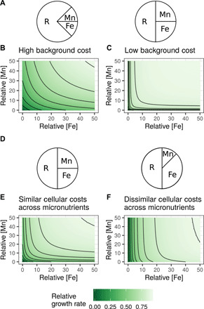
(A) A phenomenological model of a three-component proteome composed of ribosomes (R), Mn-related proteins (Mn), and Fe-related proteins (Fe). Growth rate is proportional to dFe and dMn concentrations, and micronutrients influence growth rate by removing potential resources allocated to ribosomes (see Materials and Methods for equations). (B and C) The background cost of growth (independent of Fe or Mn) can influence the apparent interaction between Mn and Fe (ΨFe equal to 0.5; see Materials and Methods for equations). Growth rate is lower overall in (B) compared with (C) because the pie charts represent ribosomal mass fraction (total protein mass in ribosomes), not number of ribosomes, and this corresponds to the parameter perturbation “amino acids per ribosome” (fig. S14). (D) The ratio of micronutrient-specific protein costs affects the apparent interaction between micronutrients (K equal to 5), as shown in (E) and (F). In (B) and (C) and (E) and (F), units are given as relative concentrations, arbitrarily ranging from 0 to 50.
Examining the ratio of cellular costs for Mn and Fe showed that maximum interdependence occurs when the cellular costs of Fe and Mn are equal (Fig. 4, D and F; Materials and Methods). For example, the internal Mn protein cost parameter had a high interaction index (fig. S14); when increased, it led to more similar protein costs between Fe and Mn. When cellular costs are similar across resources, they place similar demands on the pool of shared resources, which consequently increases their interdependence. These two mechanisms provide a tractable means to include interdependence in global ocean models because it suggests that estimating cellular costs for individual nutrients is sufficient to parameterize the overall interaction strength. We speculate that considering relative costs across resources may also apply to other nutrient pairs and help to explain previously observed patterns of interdependencies. For instance, the independent relationship between cobalamin and phosphorus (56) implies large differences in their cellular costs, whereas similar cellular costs between nitrogen and phosphorus may contribute to their interdependence (57).
Inferring in situ rates and quotas by coupling cellular modeling with metaproteomics
While our modeling framework can be combined with proteomic data to estimate the costs and constraints associated with micronutrients, this coupled approach can also be used to predict in situ biogeochemical metrics (Fig. 5A). In this way, our model is able to quantitatively reproduce growth rates under high and low dFe from a diatom culture (despite no model training on growth rate data; Fig. 5B). Using in situ dMn and dFe concentrations and metaproteomes from field samples at the Antarctic sea ice edge, in situ diatom-specific growth rates (Fig. 5C), Fe cellular quotas (Fig. 5D), and Fe uptake rates (Fig. 5E) can be estimated. These metrics are typically difficult or impossible to measure from in situ microbial communities directly but have important consequences for ocean biogeochemistry and ecosystem services. Our approach connects these rates and quotas directly with resource allocation strategies used by diatoms, highlighting a decrease in protein allocated to photosynthesis and an increase in protein allocated to iron acquisition in the transition into micronutrient stress (fig. S15), resulting in decreased growth rates and iron quotas (Fig. 5, C and D). These process-based insights are critical for characterizing the role of micronutrients in Southern Ocean phytoplankton bloom progression and fate (58).
Fig. 5. By combining cellular modeling with metaproteomic data, we inferred in situ rates and quotas.

(A) Schematic for combining environmental parameters (e.g., light and dFe), cellular modeling, and metaproteomic observations, to infer rates and elemental quotas. (B) We first demonstrated that the proteomic allocation model quantitatively reproduces growth rates from the cultured diatom T. pseudonana (45) under low and high Fe (culture data do not correspond to a posterior probability, error bars represent the standard deviation across four replicate cultures). (C to E) Coupling the metaproteome-derived diatom proteome with the cellular model, we can quantitatively infer the growth rates, iron quotas, and iron uptake rates of diatoms in these two time points from a complex microbial community. Week 1 corresponds to higher dFe and dMn, and week 3 corresponds to lower dFe and dMn [concentrations shown in (C)].
Outlook
We combined mechanistic, proteomic modeling with metaproteomics to estimate the costs and constraints associated with micronutrient-controlled growth in a polar diatom. Our results highlight the role of cellular costs rather than environmental scarcity in shaping growth, with two key factors: the internal protein cost associated with micronutrient use and the available membrane space for transporters. Identifying the differences in protein cost for vacuolar versus ferritin-based Fe storage and other micronutrient-associated costs would further connect ecological strategies with gene expression. Available membrane space has an established temperature dependence and is an important constraint on nutrient uptake kinetics [via membrane saturation (34, 59, 60)], making it critical to quantify in a changing ocean. Our approach relied on rich in situ gene expression datasets to estimate parameters, highlighting a means to quantify cellular costs and constraints.
Parameterizations of phytoplankton growth in global ocean models can have dramatic consequences for projections of ecosystem services in the context of changing upper ocean resource availability (3). Embedding a mechanistic representationof resource limitation within global ocean models will leverage rapidly expanding “omics” datasets to improve predictions of growth responses to environmental change. Developing phenomenological models to represent the outcomes of mechanistic cellular models is a tractable next step. In this way, mechanistic modeling can provide the biological flexibility and realism (61) necessary for predicting potential tipping points in ecosystem services. Mechanistic cellular models, in conjunction with in situ gene expression measurements and biogeochemical models, will improve projections of ecosystem services and further characterize the biological underpinnings of nutrient limitation in the changing ocean.
MATERIALS AND METHODS
Model description
We developed a coarse-grained model of intracellular protein allocation in the polar diatom F. cylindrus (24), extending coarse-grained kinetic models previously developed for a range of prokaryotes (25, 29–31). Uniquely, we considered micronutrient controls on proteomic allocation and applied these principles to a eukaryotic phytoplankton. We used Bayesian optimization to determine the optimal proportion of ribosomes synthesizing different coarse-grained proteomic pools to maximize the steady-state specific growth rate. The cost of producing a given coarse-grained pool is a function of the protein length or the sum of protein lengths (in units of amino acids) within a pool. Specifically, the rate of synthesizing one unit of a protein pool is inversely related to the number of amino acids per pool. The units of each intracellular variable (metabolites, proteins, and free metal pools) are in molecules per cell. As in (25, 31), we used a photosynthetic model (62) to parameterize energy production rate and similarly calculated a biosynthesis-specific growth rate. We first provide a high-level overview of the model structure and then give detailed descriptions of parameterizations.
System of equations
The dynamics of each internal metabolite and protein pool are described using a differential equation, all with growth rate as a loss term (25). The internal free manganese pool (Mni) increases with Mn uptake rate (VMn) and decreases with PSU protein synthesis (photosystem unit, γP) at a fixed stoichiometry (φMn,P) and antioxidant protein synthesis (γA) at a fixed stoichiometry (φMn,A). We solve this system of equations by integrating them forward in time to a pseudo-steady state (described in more detail in the Supplementary Materials)
| (1) |
The internal free iron pool (Fei) is controlled by protein synthesis of Fe-containing protein pools: PSUs and nitrogen metabolism. The fixed stoichiometric coefficient for PSUs is larger for Fe compared with Mn, reflecting the higher Fe demand for photosynthesis (φFe,P). Also, the nitrogen metabolism pathway (γN) requires a fixed Fe stoichiometry per pathway (φFe,N)
| (2) |
The internal free energy pool e increases with photosynthetic energy production ve, multiplied by a stoichiometric coefficient that implies a fixed number of ATP (adenosine 5′-triphosphate) and NADPH (reduced form of nicotinamide adenine dinucleotide phosphate) molecules produced per photosynthetic activation (φe). There is a small amount of energy required for Mn and Fe uptake (φTMn, φTFe) and a large energetic requirement for nitrogen metabolism (φN). The total rate of conversion of nitrate into amino acids, Vn, is subsequently used to calculate a biosynthesis-specific growth rate, where Vn is the product of TNO3 and kcat,TN. Energy is also consumed through protein synthesis. We used the sum of protein synthesis rates for each protein pool multiplied by the amino acids per pool (ηj) and multiplied the entire sum by mγ, the energetic requirement per amino acid elongation
| ( 3) |
Amino acids are produced via nitrogen metabolism (Vn); we multiplied this rate by the inverse of the average number of nitrogen atoms within each amino acid. Amino acids are then consumed by protein synthesis and diluted by growth
| (4) |
All protein pools are governed by similar dynamics, such that an increase can only arise from protein synthesis (γj) and a decrease can only arise from dilution by growth
| (5) |
| (6) |
Internal protein cost of iron and manganese
We represented the internal cost of iron and manganese by dynamically changing the Fe uptake cost per transporter (nTFe) as a function of dFe uptake rate, scaled by growth rate (i.e., ) and multiplied by a constant coefficient (θ). This approach was similarly applied to Mn uptake and Mn transporter cost. nTFe and nTMn are the uptake and internal management protein costs
| (7) |
| (8) |
Nutrient uptake kinetics
We modeled nutrient uptake rates of dFe and dMn to include both a variable maximum uptake rate and a diffusion layer (36–38, 63, 64). A flexible maximum uptake rate (i.e., Vmax) has been observed experimentally (49) and predicted theoretically (36, 65), and the diffusion layer affects the total diffusive flux to the cell surface at low bulk substrate concentrations. At high substrate concentrations (i.e., nutrient replete), the nutrient uptake rate approaches the total transporters divided by the “handling time” (h). Note that handling time (seconds per substrate) is equivalent to the inverse of the maximum turnover rate (kcat)—a commonly measured parameter in enzyme kinetics.
As the substrate concentration decreases (i.e., nutrient deplete), the uptake rate approaches the product of cellular affinity (α) and substrate concentration (S). Affinity is a function of cellular radius, the molecular diffusivity coefficient, and the proportion of cellular area covered by transporters (37). We assumed that Fe and Mn uptake can only be from the dissolved phase and used a molecular diffusivity coefficient of 0.9 × 10⁻⁹ m2 s−1 for both (66). For nitrate, we used a molecular diffusivity coefficient of 1.17 × 10⁻⁸ m2 s−1 (67), with a transporter radius of 1 × 10⁻⁹ m (36).
For modeling multiple nutrient uptake rates simultaneously, we adjusted the nutrient uptake model above by multiplying the diffusive flux term (4Dπr) by the proportion of surface area covered by other transporters not corresponding to nutrient i (ξ), where D is the diffusivity coefficient and r is the cellular radius. Given that approximately 50% of a lipid membrane must consist of phospholipids to maintain membrane integrity (68), and there is a significant requirement for macronutrient transporters, we also restrict the “available” area for iron and manganese transporters, hypothesizing that a subset of membrane area is available (κ). To model the proportion of membrane space available, we modified the diffusive flux term using the original derivation (63). Below, S is the bulk concentration of nutrient i, ni is the number of transporters for nutrient i, and s is the radius of the transporter for nutrient i. Transporters are modeled as circular planes with constant radii on a sphere (69). In addition to the uptake model (37), we included an additional Michaelis-Menten term of energy dependence
| (9) |
| (10) |
| (11) |
| (12) |
| (13) |
| (14) |
| (15) |
| (16) |
Iron speciation
At low concentrations, dFe uptake is bound by physical limits of diffusion to a cell membrane (70, 71). Under these conditions, cells are under “diffusion limitation,” as dFe uptake rates are close to the diffusive flux. These studies considered Fe uptake when only Fe′ (free, inorganic Fe) was bioavailable and Fe-EDTA is not significantly taken up by eukaryotic phytoplankton (72). Yet, in the ocean, most of the dissolved Fe is organically complexed (FeL) (73), which is, to some extent, bioavailable for uptake. We therefore included both sources of iron for uptake. While a large portion of the dFe pool is likely bioavailable, not all dFe species are equally bioavailable (74, 75). Ligand-bound Fe has maximum uptake rates roughly three orders of magnitude lower than Fe′ (48, 72, 74). We modeled dFe uptake by splitting the dFe pool into subcomponents of Fe′ and FeL, and then summing the uptake rates. This formulation assumes that phytoplankton in the ocean are simultaneously under diffusion and “ligand exchange” limitation (71). This can be extended to any number of distinct dFe pools with corresponding uptake rate characteristics. Fe′ would primarily be controlled by diffusion limitation and is limited by the chemistry and physics of diffusion to the cell surface and, therefore, only affected by α (which is a function of the cell radius, r, diffusivity coefficient of dFe, D, and the proportion of cell surface area covered by transporters). FeL uptake (ligand exchange limitation) is limited by the rate constants of uptake (i.e., the handling time) and the number of transporters.
We first split the dFe pool into Fe′ and FeL, by multiplying the bulk concentration of dFe by 2 and 98%, respectively (71). We then use separate kinetic constants, where the maximum turnover rate per transporter of the FeL pool is kcat, Fe′ × 10−3.
Consequences of reactive oxygen species
ROS can hamper photosynthesis by negatively affecting protein synthesis (76). We aimed to capture an overrarching consequence of ROS in phytoplankton cells in this model—damaged proteins. Cells can combat ROS production by producing antioxidants, such as superoxide dismutase (e.g., Mn/FeSOD), or alternatively manage the consequences by resynthesizing damaged proteins. We represented this trade-off in the model by “leaking” a proportion of energy synthesis from PSUs into superoxide. Superoxide is represented implicitly in the model structure and not as an internal pool. Superoxide is produced from electrons leaked by photosynthetic energy production and consumed by MnSOD. Excess superoxide that is not consumed by SOD then penalizes the maximum protein synthesis rate, while overinvestment in SOD diverts protein synthesis away from other protein pools. We also model the relationship between electron leakiness and Fe quota (proportion of electrons leaked is ϵp below), as previous work suggests that the tendency of an electron to be donated to molecular oxygen increases under Fe stress.
Oxidative stress can result from a mismatch between ROS consumption rate (via antioxidants) and production rate (electron transport). We modeled ROS consumption rate as the product of the maximum turnover rate of MnSOD (kcatROS, MnSOD) and the number of MnSOD copies per cell (A). The rate of ROS production is a proportion (ϵp, see below) of energy production (ve). Higher rates of energy production require increased investment in MnSOD. The ϵa parameter represents the efficacy per MnSOD and is empirically estimated (described below)
| (17) |
| (18) |
| (19) |
An imbalance between production of ROS and available MnSOD (ω) decreases the maximum protein synthesis. We represented this phenomenologically by multiplying the protein synthesis rate by a value ranging from 0 to 1 (pw). A phenomenological variable R0 is used here with a value of 10
| (20) |
Electrons that are leaked not only produce ROS but also decrease energy production (fewer electrons can be used to create ATP or NADPH). We therefore modified the photosynthetic electron production term above by the proportion of leaked electrons
| (21) |
Photosynthetic energy production
We used a previously published photosynthetic model (25, 62). This model assumes a two-state configuration of photosystem units. We obtained an expression for energy production [as in (25)], by writing this model as a system of two ODEs, where the inactivated PSUs are synthesized (γP), and both inactivated (P0) and activated PSUs (P*) are diluted via growth (μ). The rate of PSU activation is v1, and the rate of switching back to an inactive PSU is ve
| (22) |
| (23) |
The rate of PSU activation is a function of the absorption cross section (σ), the amount of irradiance (I), and the amount of inactivated PSUs. The rate of conversion from activated to inactivated PSUs is a function of electron turnover rate (τ)
| (24) |
| (25) |
We can then assume a pseudo-steady state between the inactivated and activated PSUs and solve for the energy production rate (ve)
| (26) |
Calculating growth rate
We calculated growth rate as in (25) with some slight modifications. We calculated a biosynthesis-specific growth rate (13, 25, 30) by calculating the rate of biosynthesis relative to the average protein mass per cell. We assumed a fixed average protein mass per cell (Mcell), using data from (77) [from file S1 in (77)] for the median picograms of protein per cell from Pseudonitzschia, which is converted to amino acids per cell. In our model, biosynthesis rate is represented as the conversion of nitrate into amino acids. Total biosynthesis rate (Vn) is equal to the number of biosynthetic pathways multiplied by rate-limiting enzyme maximum turnover rate (see the “Model parameterization” section)
| (27) |
A proportion of the proteome is considered growth rate independent (78). We included a fixed proteomic pool (Λ) in our model that represents “maintenance metabolism”—respiration, lipid biosynthesis, etc. This is modeled by multiplying the total protein per cell by a constant proportion. We assumed that 20% of the proteome is growth rate independent (79), although future research is required to determine this value in eukaryotic phytoplankton
| (28) |
Relationship between Fe quota and electron leakage
Previous research suggests that the tendency of an electron to be donated to molecular oxygen increases under Fe stress (32). We represented this increased leakiness by designating the proportion of electrons leaked to molecular oxygen, ϵp, as a function of the total cellular Fe quota. We constrained this from 5 to 30% using observations of total Fe to carbon ratios observed in the SOFEX cruise (47), with a range of 5.5 to 30 μmol Fe:mol C. Then, by using carbon-to-volume ratios from (80), we converted the lower and upper bounds of μmol Fe:mol C to a total cellular quota (Fe atoms per model cell). A linear relationship between ϵp and total Fe quota was assumed when the Fe quota is within these observationally constrained bounds. Below the minimum Fe cell quota, ϵp is fixed at 30%; above the maximum Fe cell quota, ϵp is fixed at 5%. This corresponds to the following relationship
| (29) |
Protein synthesis
Protein synthesis connects the internal pools of metabolites and free micronutrients to proteins
| (30) |
| (31) |
| (32) |
| (33) |
| (34) |
| (35) |
| (36) |
In the equations above, γmax refers to the maximum protein synthesis rate, which is a function of temperature (degrees Celsius) with a Q10 value of 2 (18). We calculate a ROS-adjusted protein synthesis rate, γROS, by multiplying the temperature-adjusted protein synthesis rate by pω (ranging from 0 to 1). Protein synthesis to protein pool j (γj) is a function of the proportion of ribosomes allocated (βj), the protein cost (ηj; larger protein pools have a slower rate of synthesizing one unit), the number of ribosomes (R), and the availability of energy (e) and amino acids (aa). Furthermore, those protein pools that have cofactor requirements have an additional Michaelis-Menten term. All half-saturation constants (Ke, Kaa, KFei, and KMni) used for internal metabolites were set to an arbitrarily low value of 104 molecules per cell (implying efficient allocation of resources within the cell).
Model parameterization
We used the BRENDA database to search for kinetics constants. For the protein lengths, we examined the F. cylindrus genome (24) and searched for protein coding genes with Gene Ontology (GO) terms corresponding to our coarse-grained pools. Generally, the protein cost reflected the length of all proteins within a coarse-grained protein pool. Photosynthetic-specific parameters were taken from previously published datasets.
Ribosomal proteins
To estimate the total proteomic cost per ribosome, we used data from the model alga Chlamydomonas reinherdtii. In C. reinherdtii, 96 proteins were estimated for cytosolic ribosomes (81). These proteins ranged in size from 12 to 54 kDa. Assuming an average size of 33 kDa, this converts to a protein cost of 3168 kDa (3,168,000 Da), or 28,800 amino acids (using the average molecular mass per amino acid, 110 Da). We therefore used 28,800 amino acids per ribosome as the fixed protein cost.
Photosynthetic proteins
Our protein cost per photosystem unit was taken as 12,177 amino acids per PSU (82), assuming a 1:1 architecture of PSII:PSI. We used the reported approximate molecular mass per photosystem unit (1339.5 kDa) and converted that to amino acids using the average molecular mass per amino acid (110 Da).
Fe and Mn transporters
We searched the F. cylindrus genome for the GO term “iron ion transport” (GO:0006826). We used the sum of unique proteins identified with this search, excluding ferritin, as we explicitly model that protein (see above). We acknowledge that this approach crudely approximates the protein requirements for Fe uptake, as the exact protein stoichiometry and the specific combination of proteins required are still unclear. We also included the average of the four copies of FBP1 identified in F. cylindrus (83). The total cost per transporter for Fe uptake was 4028 amino acids.
Four natural resistance-associated macrophage proteins (NRAMPs) were identified as manganese transporters in the F. cylindrus genome (84). The average protein length per NRAMP was 372 amino acids.
Nitrate uptake and amino acid biosynthesis
We represented the transformation pathway from nitrate to amino acids as the core iron-dependent biosynthetic cellular pathway. This pathway is represented in our model as a single unit with high protein, energetic, and iron costs. We combined the protein lengths of nitrate transporters (NRT2 transporters), nitrate reductase (represented as a homodimer), nitrite reductase, glutamine synthetase, and glutamate synthase, which sum to 5893 amino acids per pathway.
At substrate saturating conditions assuming fixed pathway stoichiometry, the enzyme in a pathway with the lowest maximum turnover rate (kcat) determines the upper bound on pathway flux. We used this “kinetic bottleneck” approximation to describe the conversion of nitrate into glutamine. For the enzymes described above, we found that glutamine synthetase had the lowest kcat for NH4 [2.96 s−1 , Enzyme Commission no. 6.3.1.2 (85)], and we therefore use this value to represent the rate-limiting step.
We approximated the energetic requirement for the entire conversion by summing up the ATP and NADPH cofactors required for each step in the synthesis of glutamine from imported nitrate. We accounted for one ATP from nitrate uptake, one NADPH for nitrate reduction, one NADPH for nitrite reduction, one ATP for glutamine synthetase, and one NADPH for glutamate synthase. Assuming an interconversion ratio of 2.6 ATP to 1 NADPH, the total energetic cost was 9.8 e.
For the Fe requirement in this pathway, we summed up the per-enzyme atoms of Fe. We accounted for two Fe atoms in nitrate reductase (one per subunit, but it exists as a homodimer), five Fe atoms in nitrite reductase in total (one siroheme cofactor and four in the 4Fe-4S cluster), and three Fe atoms in glutamate synthase. Thus, the total stoichiometric coefficient for this pathway is 10 Fe atoms (φFe, N).
Uptake rate kinetic constants
To obtain kinetic constants for Fe transporters, we leveraged previously published data and methods for inferring maximum uptake rate per transporter. Hudson and Morel (70) derive a kinetic constant for the maximum turnover rate per transporter, equivalent to the inverse of the handling time, by using pulse chase experiments with labeled Fe. They assume that the whole-cell response of uptake kinetics approximates that of the kinetic constant of the transporter, which, in other words, means that there is no downstream regulation of Fe uptake beyond that of the transporter (i.e., internalization kinetics and saturation). Yet, enzyme kinetics can be regulated at the pathway level (86); therefore, we challenge the assumption of no downstream regulation from Fe uptake. Comparing the magnitude of the maximum turnover rate per transporter reported in (70) to other nutrient transport kinetics, but derived differently (38), suggests that using pulse chase experiments to estimate transporter kinetic constants underestimates these constants because of downstream inhibition. However, (70) still provides invaluable measurements of cell-specific uptake rates that can be used to infer kinetic constants.
We leveraged published uptake rate data (70) and recalculated the maximum turnover rate using a method described in Eq. 16 (38). This resulted in a kin value approximately three orders of magnitude higher than inferred in (70), which was much more similar to values estimated for macronutrient transporters (38). We used the following values from (70) to recalculate the handling time: a maximum uptake rate (Vmax) of 180 amol cell−1 hour−1, a half saturation constant (Km) of 3.1 nM, a diffusion coefficient (D) of 5.4 ×10⁻⁸ m2 min−1, a cell radius (r) of 5.6 ×10⁻⁶ m, and a transporter size (s) of 1−9 m.
Protein synthesis parameters
We used the translation rate from Thalassiosira weissflogii at 20°C of 1.9 amino acids per ribosome per second (18). Assuming a temperature dependence given by a factor of Q10 equal to 2 (18), protein synthesis rate is adjusted in the model according to the input temperature (−1°C for the metaproteomic conditions). For the energy required per amino acid elongation, we used the equivalent of 3 e units (25).
Photosynthetic parameters
We needed two parameters for the photosynthetic energy production model: the absorption cross section and the rate of returning from an activated PSU to an inactivated PSU (τ). For the absorption cross section, we used a value of 0.01 m2 μE−1 (87), and for the PSU turnover rate, we used a value of 6000 min−1 (88).
Culture diatom comparison
We used two published diatom datasets that examined how Fe influences the proteome (44, 45). The observed protein data from both datasets were manually binned into our corresponding model coarse grains. For (45), we used the sum of spectral counts per peptide as an approximation for the mass per protein group. For (44), we used the reported normalized spectral abundance factor values per protein. Note that while both of these datasets used diatoms (44, 45), the studied diatoms were Thalassiosira pseudonana and P. granii, and our model is based off of the polar diatom F. cylindrus.
To compare the model predictions under these laboratory conditions, we also modified the temperature and light level inputs to the model to reflect the culture conditions. The Fe levels in culture were set with EDTA, and most Fe taken up in culture with FeEDTA is inorganic free Fe. Therefore, we changed the Fe speciation input to reflect this, such that there is only a small available FeL pool (1%), while the inorganic free Fe pool was set to 99% of total dFe.
Southern Ocean Mn, Fe, and light conditions
FISH data
Surface seawater (approximately 3-m depth) was pumped from a tow FISH into a clean container using a Teflon diaphragm pump (Almatec A15) connected to a clean oil-free air compressor (JunAir) and GEOTRACES cruise JR274 (89).
Concentrations of trace metals were determined by isotope dilution inductively coupled mass spectrometry (ICP-MS), while the monoisotopic elements Co and Mn were analyzed using a standard addition approach followed by ICP-MS detection, all according to methods described in (90). The ICP-MS analyses were conducted following an off-line preconcentration/matrix removal step (90) on a Wako chelate resin column (91).
GEOTRACES data
We used the GEOTRACES intermediate data product (92) to determine average Mn and Fe concentrations within the mixed layer for cruise stations in the Southern Ocean. To calculate the mixed layer depth, we calculated the potential density at 10 m and determined the depth at which this 10-m potential density is 0.03 kg m−3 more dense (93). For each station, we used the discrete data product and averaged the Fe and Mn concentrations above the mixed layer depth.
We also calculated the median light level (photosynthetically active radiation, PAR) within the mixed layer. We used monthly climatology of surface PAR and diffuse attenuation coefficient (Kd490) from the Ocean Color database from 2002–2018. The median mixed layer light levels were determined using the surface PAR, Kd490 and mixed layer depth (94)
| (37) |
where MLD is the inferred mixed layer depth and I0 is the surface irradiance.
Metaproteomic sampling and LC-MS/MS
We sampled the microbial community at the sea ice edge in McMurdo Sound, Ross Sea at the same location (−77.62S, 165.41E) for 4 weeks [as described in (28)]. We had four sampling dates corresponding to weeks 1 to 4: 28 December 2014 and 6, 15, and 22 January 2015. Large volumes of water (150 to 250 liters) were filtered from 1-m depth at the sea ice edge and passed through three filters sequentially (3.0, 0.8, and 0.1 μm, each 293 mm Supor filters). Filters with collected biomass were then placed in tubes with a sucrose-based preservative buffer [20 mM EDTA, 400 mM NaCl, 0.75 M sucrose, and 50 mM tris-HCl (pH 8.0)] and stored at −80°C until sample processing. We extracted proteins after buffer exchange into a 3% SDS solution as previously described (28).
To prepare samples for liquid chromatography tandem mass spectrometry (LC-MS/MS), the precipitated protein was resuspended in 100 μl of 8 M urea, and then we ran a Pierce bicinchoninic acid protein assay kit (Thermo Fisher Scientific) to quantify the protein concentration in each sample. We then reduced the protein sample using 10 μl of 0.5 M dithiothreitol and incubated the sample for 30 min at 60°C. Samples were then alkylated using 20 μl of 0.7 M iodoacetamide in the dark for 30 min, diluted with 50 mM ammonium bicarbonate, and digested with trypsin using a 1:50 trypsin:protein ratio. We then acidified [1.5 μl of trifluoroacetic acid (TFA) and 5 μl of formic acid added] and desalted samples. We desalted the samples by first conditioning the solid-phase columns with methanol (1 ml), then 50% acetonitrile (ACN) and 0.1% TFA, and then 2× 1 ml of 0.1% TFA. Samples were loaded onto columns that were subsequently washed 5× with 1 ml of 0.1% TFA. Last, peptides were eluted from the columns with 2× 0.6 ml of 50% ACN and 0.1% TFA, and 1× 0.6 ml of 70% ACN and 0.1% TFA.
We used a one-dimensional LC-MS/MS to characterize the metaproteome. For the largest filter size (3.0 μm), we used three injections per sample and two injections per sample for the 0.8- and 0.1-μm filters. We ensured that the protein concentration in each urea-resuspended sample was equivalent across sampling weeks and within each filter size. We used an LC gradient from 0 to 10.5 min with 0.3 μl/min flow of 5% solution B; from 10.5 to 60 min, the flow was 0.25 μl/min, and solution B increased to 25.0%; from 60 to 90 min, %B increased to 60%; from 90 to 97 min, %B increased to 95%; from 97 to 102 min, %B remained at 95%; from 102 to 105 min, the flow rate increased to 0.3 μl/min and %B decreased to 5% for 20 min. Solution A is 0.1% formic acid in water, and solution B is 0.1% formic acid in ACN. Peptides were injected onto a 75 μm × 30 cm column (New Objective, Woburn, MA) self-packed with 4 μm, 90 Å, Proteo C18 material (Phenomenex, Torrance, CA), and then online LC was performed using a Dionex Ultimate 3000 UHPLC (Thermo Fisher Scientific, San Jose, CA).
We used a data-dependent acquisition approach with a VelosPRO Orbitrap mass spectrometer (MS; Thermo Fisher Scientific, San Jose, CA) to characterize the metaproteome for each sample. We used an MS method with the following parameters: dynamic exclusion enabled, with an exclusion list of 500 and an exclusion duration of 25 s; a mass/charge ratio (m/z) precursor mass range from 300 to 2000 m/z; and a resolution of 60,000. MS2 scans were collected with a TopN method (N = 10), using collision-induced dissociation with a normalized collision energy of 35.0, an isolation width of 2.0 m/z, a minimum signal of 30,000 required, and a default charge state of 2. Ions with charge states less than 2 were rejected, and those above 2 were not rejected. Last, we used polysiloxane as a lock mass.
For a database of potential proteins present, we used a metatranscriptome obtained from a nutrient incubation experiment conducted using water collected during week 2 of protein sampling (40). Before database searching, we removed all redundant protein sequences (P. Wilmarth, fasta-utilities) and appended the cRAP (Global Proteome Machine Organization common Repository of Adventitious Proteins) database of common laboratory contaminants. We then applied a Savitzky-Golay noise filter, a baseline filter, and applied a high-resolution peak picking approach to centroid the MS data (95). To identify peptides, we conducted a database search with MSGF+ (96). We used a 1% false discovery rate at the peptide-spectrum match level. Once we had identified peptides within each MS injection, we quantified these peptides at the MS1 level using the “FeatureFinderIdentification” approach (97), where peptides identified in one injection can aid identifying peptides in a different injection without corresponding MS2 spectra. In this approach, the user must identify a group of samples across which peptides can be cross-mapped. We grouped our samples by filter sizes, with replicate injections also within each group for cross-mapping. Mass spectrometry mzML files within each group were then aligned using MapAlignerIdentification (95), and then we applied FeatureFinderIdentification to obtain peptide-specific MS1 intensities. Once peptides were quantified for each injection, we then obtained a sample-specific peptide quantity, which was the average peptide-specific intensity across injections. We only used this quantity if a given peptide was observed across all injections.
We then mapped peptides to taxa and to protein functions. Peptides were mapped to taxa only if they uniquely correspond to a given taxonomic group. Coarse taxonomic groups (presented at the phylum level) were chosen because coarse-graining is robust to various MS-induced biases (43). We suggest that the sum of taxon-specific peptide abundances (MS1 intensities in this case) can be used as a proxy for biomass. To evaluate this approach, we used a previously published, artificially assembled metaproteome (42). In this dataset, we identified all taxon-specific peptides and then examined the correlation between the amount of protein used for a taxonomic group and the sum of peptide intensities that correspond to that taxa. We found a high correlation between the sum of peptide intensities and the total protein (fig. S1). In addition, we examined different MS chromatographic methods [data files “Run1and2_U1.pep.xml” and “Run4and5_U1.pep.xml” from (42)]. We show that there is a high correlation between the amount of protein and the sum of peptide intensities across three orders of magnitude (fig. S1), and this correlation is higher in the longer chromatographic run.
Mapping peptides to taxon-specific functional groups has additional challenges because there can be multiple functional labels for a given protein, and the functional label can differ on the basis of the annotation used. To address this issue, we used five different functional annotations [KEGG (Kyoto Encyclopedia of Genes and Genomes), KO (KEGG Orthology), KOG (Eukaryotic Orthologous Groups), Pfam, and TIGRFAM annotations (98–102)] and mapped coarse-grained functional associations by matching a list of strings, i.e., keywords (which were identified in the construction of the model). In addition, we manually examined the matched proteins to ensure we were not capturing incorrectly mapped proteins to coarse grains.
ABC for parameter estimation
Metaproteomic-to-model data comparison
To infer parameters of the model given the proteomic data, we need to determine how similar the observations are to the model predictions. However, there are several challenges associated with comparing the proteomic data with the protein allocation model output. The main challenge with doing a direct comparison of model output (i.e., with protein mass fraction) is the components of the observed proteome that we are not modeling. For example, we do not include DNA synthesis proteins in our cellular model, yet we anticipate this protein mass fraction to vary with growth rate. The consequence of this issue is a poor model fit, which can hamper parameter inference.
We propose a general approach to address this challenge using the ratio of the protein pool abundance from the two conditions observed. By using this ratio, we can still capture the change in protein expression across conditions, but we bypass the issue of the nonmodeled proteome. Specifically, we used the ratio of protein group abundance from the low Fe to high Fe condition in the culture diatom proteomes, and the third sampling point to the first sampling point from the metaproteomic time series. This general approach for model-to-metaproteome comparisons might be useful in other contexts, as we anticipate this issue would be pervasive, because no proteomic allocation model can explicity include all proteins synthesized.
There are also several transformations and considerations required to make comparisons between the model and the observations. The first transformation is to calculate protein mass fraction from the model. The true mass fraction from our model considers the free amino acid pool, yet this pool would not be observed using typical proteomic methods. Thus, we first recalculate the total observable protein mass from the model. This is done by multiplying all protein abundances by the amino acids per protein pool. For Fe and Mn uptake, this cost is dynamic, so we recalculate the dynamic cost per transporter and internal machinery first. Once we have recalculated protein mass, the next consideration is the observed proteins. This is straightforward for all the protein pools except for Fe and Mn uptake and internal cost. This is because the observed proteins for this protein pool can be considered part of the internal or external protein pool (or both). For each of the datasets, we examined the Fe transporters and internal Fe cost proteins and determined whether it is appropriate to use the external or internal protein pool from the model as a comparison. We did not observe ferritin in any dataset; the main protein observed for this protein pool was phytotransferrin (ISIP2a). We considered phytotransferrin to be both an internal and an external cost, given that the protein is endocytosed (48). These transformations for each dataset enabled a careful comparison between the data and the observations.
ABC for parameter inference
We used ABC to draw inferences about the three unconstrained parameters in the model: the efficacy per MnSOD, ϵa; the available space on the membrane for Mn and Fe transporters, κ; and the internal Fe and Mn cost coefficient, θ. Note that we assumed that θ is constant for both Mn and Fe, although with additional data, we would be able to further discriminate across these costs.
We used ABC to obtain a posterior distributions for parameters and predictive distributions for observed data. The stochastic model was combined with our cellular model to allow for errors in approximation. To obtain a posterior distribution for each parameter, we accounted for error in the model and observations. Specifically, our cellular model (f) generates observations (yi) from a vector of parameters [νi = (ϵai, κi, θi)]. We included an error term (ei), which we assume is normally distributed with a common standard deviation (h)
| (38) |
| (39) |
We treated the standard deviation h as fixed, and estimation of the posterior distribution is described below. The priors for the elements of ν = (ϵa, κ, θ) were independently uniform, ϵa ∼ U(0.00001,0.1), κ ∼ U(0.001,16), and θ ∼ U(0.001,0.15). For ϵa, we drew from a uniform bounded by 0.00001 and 0.1, because initial tests suggested that this range resulted in a Mn:Fe ratio and a Mn-PSU:Mn-SOD ratio consistent with empirical observations (45). For θ, we drew from a uniform bounded by 0.001 and 16. The upper bound assumes that all internal Fe is stored in ferritin, which would result in a very high internal Fe cost. The lower bound represents an arbitrarily low protein cost. For κ, we used a lower bound of 0.001 and an upper bound of 0.15. We hypothesized that the proportion of membrane space available for Fe and Mn transporters is likely within these bounds, considering that only approximately 50% of the membrane can even have transporter proteins (68), and there must be a large proportion dedicated to macronutrient transporters.
We used an ABC algorithm to approximate the exact posterior (39, 103). The approach simulates ν1, …, νB from the uniform priors and then generates y1 = f(ν1), …, yB = f(νB) from the cellular model. For each yi, a weight wi(h) ∈ {0,1} is generated from a Bernoulli distribution [ai(h)] where
| (40) |
For any function g(ν), its posterior expectation is approximated by
| (41) |
We can determine P(νj ≤ t∣y0) at each point along the grid and then convert these estimates from a cumulative distribution to a probability density. We do so by calculating the height of the kth bin [tk − 1, tk] as
| (42) |
Intuitively, if the Euclidean distance of a simulated dataset yi to y0 is very low, then it is very likely that the parameter vector νi would be included in the posterior. This approach gives an approximation of E[g(ν)∣y0] with a fixed and known h. We then conducted the posterior sampling M times to infer the approximate posterior distribution at fixed intervals (i.e., the posterior as a histogram, with M = 400,000). Overall, this method allows for a probabilistic sampling of the posterior, as we transform our deterministic model output to a stochastic model, with the stochasticity coming from the error term (39). Without this step, our posterior variance estimates would solely be a function of the tolerance that we use for inclusion in an approximate posterior (104).
After sampling from the prior distribution (182,171 samples drawn), we ran the cellular model and generated a set of model outputs for each of three datasets: the metaproteome-derived diatom proteome at two time points with corresponding in situ dMn and dFe concentrations, T. pseudonana proteome under high and low Fe (45), and P. granii diatom proteome under high and low Fe (44). We then compared the model output with each of these datasets, and the success probabilites given above are calculated by combining observations and model predictions across all three datasets. We combined these datasets to estimate the first-order effects; however, it is possible that the parameters included are environment dependent. For example, the temperature is different across each dataset, yet we assume that the membrane space parameter (κ) is from a single distribution. Numerical integration and optimization parameters were adjusted to enable faster sampling of parameter space; specifically, we shortened the integration time to a length of 1 × 10⁶ (with steps of 10). Optimization settings are given in the Supplementary Materials.
Estimating standard deviation of the error term: h
The standard deviation of the error term, h, is an important parameter for conducting ABC. This error term encompasses error from mass spectrometry, sample processing, and natural biological variability. We empirically estimated this parameter by using culture replicates from (45). We calculated the average standard deviation of the ratio of protein pools across replicates. To do so, we randomly paired biological replicates and determined the sample standard deviation
| (43) |
We inferred an average sample standard deviation (across all pairs of biological replicates) of 0.007. However, with such a low standard deviation, our ABC approach was not feasible because the probability of acceptance was so low across all parameter vectors. We therefore increase the value of h to a conservative value of 2, likely overestimating the standard deviation of the error distribution.
Model settings, parameter perturbation experiments, and interaction index
We generated model output for a range of dFe and dMn values: 1, 50, 100, 500, 1000, 2000, and 3000 pM in a full factorial combination, with light levels set to 50 μE m−2 s−1. For the three unconstrained parameters (described above), we used the modes of their posterior probability distributions for the inferred parameter value. We then conducted 20 replicate model runs for each unique combination of dFe and dMn with the following settings: nitrate at saturating conditions (input nitrate set to arbitrarily high concentration of 1 × 10⁹ nM; note that our kinetic bottleneck approximation is satisfied only under saturating conditions) and an integration time 3 × 10⁶ for the second stage of optimization (with steps of 10; see the Supplementary Materials for additional details on optimization settings).
We multiplied every parameter individually by 5 and examined the change in growth rate (except the “Fixed Proteome Percentage” parameter, which was divided by 5 because the base value was 20%). Each perturbation experiment was conducted three replicate times, and the average growth rate of these three was then divided by the base model (i.e., with no parameters altered, also run three times). Four environmental conditions were chosen for parameter perturbation experiments, corresponding to high and low dFe and dMn (all combinations of these conditions). The high dFe and dMn conditions were set to 3000 pM. The low conditions were determined by fitting a Monod-style growth function to modeled growth rates (figs. S11 and S12) and then using the half-saturation constants. For dMn, this corresponded to 1.42 pM, and for dFe, this corresponded to 88.9 pM.
We used the parameter perturbation experiments and the following equation to obtain a quantitative metric of how different cellular processes contribute to interdependence between dFe and dMn (μ corresponds to the growth rate)
| (44) |
A phenomenological model of nutrient interdependence
Scott et al. (13) develop a phenomenological model connecting growth rate with gene expression. We extended a similar framework to micronutrients and explored interdependence across elemental metabolisms using this framework. Consider a three-component proteomic model, ϕR (ribosomal mass fraction), ϕFe (Fe-metabolism protein mass fraction), and ϕMn (Mn-metabolism protein mass fraction). Scott et al. (13) suggest that
| (45) |
Under high micronutrient concentrations, we anticipate that the proteomic mass fraction required to acquire these nutrients decreases, such that ϕFe and ϕMn are inversely proportional to the amount of dFe and dMn
| (46) |
| (47) |
It follows that the increased mass fraction required for processing and obtaining Fe and Mn negatively influences the growth rate via decreasing the ribosomal mass fraction (ϕR)
| (48) |
If we then assume a saturating function of the proteomic mass fractions (ϕFe,Mn) dependent on the micronutrient concentration
| (49) |
where K is the half saturation constant for Fe and is equivalent (for simplicity) to the half saturation for Mn. We then obtain an expression for the growth rate
| (50) |
However, the expression above requires some proteomic cost weighting factor; otherwise, the expression could result in negative growth rates. If we define the proteomic cost weight for Mn and Fe to be ψMn and ψFe, we obtain
| (51) |
| (52) |
We found that when protein costs have similar values for Fe and Mn (i.e., ψFe is 0.5), the apparent amount of interdependence is greatest. This is demonstrated by looking at the gradient of the growth rate function with respect to dMn and dFe
| (53) |
If we then assume that both dFe and dMn are at concentrations equivalent to their half-maximal growth (i.e., K), the gradient function then simplifies to
| (54) |
From this function, we can then show that the direction that corresponds to the most elemental interdependence is when the slope is closest to 1, or that the elements of the gradient with respect to dFe and dMn are equivalent. When we equate the elements of the gradient, evaluated when dFe and dMn are at half-maximal growth, we find that the iron cost parameter is equivalent to 0.5, and therefore, so is the manganese cost parameter. This phenomenological model suggests that when the ratios of proteomic costs are similar, the extent of elemental interdependence is greatest. Note that “proteomic” cost in this case can be extended to other cellular costs, for example, available membrane space.
Acknowledgments
We are grateful to N. Youssef and L. Jabre for discussions and comments on the manuscript. We thank A. Cohen from the Dalhousie Biological Mass Spectrometry Core Facility for assistance with mass spectrometry data acquisition, Compute Canada for computational resources, the Ocean Biology Processing Group for data, L. Jabre for help with Fe′ calculations, M. Faizi for correspondence about the modeling framework, and A. Sawatzky for assistance with schematic in Fig. 5A. We thank D. Hutchins, J. Hoffman, R. Sipler, J. Spackeen, and D. Bronk, as well as Antarctic Support Contractors and the staff at McMurdo Station for support in the field. Funding: J.S.P.M. acknowledges support from the NSERC CREATE Transatlantic Ocean System Science and Technology Program and the Killam Scholarship. This project was financially supported by NSERC Discovery Grant RGPIN-2015-05009 to E.M.B.; Simons Foundation Grant 504183 to E.M.B.; an NSERC CGS Postgraduate scholarship to J.S.P.M.; European Research Council (ERC) under the European Union’s Horizon 2020 research and innovation programme (grant agreement no. 724289) to A.T.; NSF-ANT-1043671, NSF-OCE-1756884, and Gordon and Betty Moore Foundation Grant GBMF3828 to A.E.A.; and a Google Cloud Research Credit Grant to E.M.B. E.S. was supported by a Discovery Grant from NSERC. Author contributions: J.S.P.M., A.T., E.P.A., and E.M.B. conceived the study; J.S.P.M. wrote all the code and conducted all analyses and lab work, with input from A.T., E.P.A., E.S., and E.M.B.; E.S. specifically contributed to the design of the ABC analysis; E.P.A. contributed data with Southern Ocean trace metal concentrations; E.M.B. and A.E.A. conducted the Antarctic sample collection and generated the reference metatranscriptome and annotation; J.S.P.M., A.T., E.P.A., and E.M.B. wrote the paper with input from E.S. and A.E.A. Competing interests: The authors declare that they have no competing interests. Data and materials availability: All data needed to evaluate the conclusions in the paper are present in the paper and/or the Supplementary Materials, and all data are publicly available. Model runs, experiments, and output from metaproteomic bioinformatics are deposited in Dryad and can be found at https://doi.org/10.5061/dryad.xd2547dfs. Model parameters used are provided in a table (table S1) in addition to being described in the Supplementary Information. The mass spectrometry proteomics data have been deposited to the ProteomeXchange Consortium via the PRIDE partner repository with the dataset identifier PXD022995 (105). Code for all metaproteomic analyses is available from https://github.com/bertrand-lab/ross-sea-meta-omics, and code for all other analyses is available from https://github.com/bertrand-lab/mn-fe-allocation.
SUPPLEMENTARY MATERIALS
Supplementary material for this article is available at http://advances.sciencemag.org/cgi/content/full/7/32/eabg6501/DC1
REFERENCES AND NOTES
- 1.Field C. B., Behrenfeld M. J., Randerson J. T., Falkowski P., Primary production of the biosphere: Integrating terrestrial and oceanic components. Science 281, 237–240 (1998). [DOI] [PubMed] [Google Scholar]
- 2.Tagliabue A., Bowie A. R., Boyd P. W., Buck K. N., Johnson K. S., Saito M. A., The integral role of iron in ocean biogeochemistry. Nature 543, 51–59 (2017). [DOI] [PubMed] [Google Scholar]
- 3.Tagliabue A., Barrier N., du Pontavice H., Kwiatkowski L., Aumont O., Bopp L., Cheung W. W. L., Gascuel D., Maury O., An iron cycle cascade governs the response of equatorial Pacific ecosystems to climate change. Glob. Chang. Biol. 26, 6168–6179 (2020). [DOI] [PubMed] [Google Scholar]
- 4.Assmy P., Smetacek V., Montresor M., Klaas C., Henjes J., Strass V. H., Arrieta J. M., Bathmann U., Berg G. M., Breitbarth E., Cisewski B., Friedrichs L., Fuchs N., Herndl G. J., Jansen S., Kragefsky S., Latasa M., Peeken I., Rottgers R., Scharek R., Schuller S. E., Steigenberger S., Webb A., Wolf-Gladrow D., Thick-shelled, grazer-protected diatoms decouple ocean carbon and silicon cycles in the iron-limited Antarctic Circumpolar Current. Proc. Natl. Acad. Sci. 110, 20633–20638 (2013). [DOI] [PMC free article] [PubMed] [Google Scholar]
- 5.Twining B. S., Baines S. B., The trace metal composition of marine phytoplankton. Annu. Rev. Mar. Sci. 5, 191–215 (2013). [DOI] [PubMed] [Google Scholar]
- 6.Saito M. A., Goepfert T. J., Ritt J. T., Some thoughts on the concept of colimitation: Three definitions and the importance of bioavailability. Limnol. Oceanogr. Lett. 53, 276–290 (2008). [Google Scholar]
- 7.Kafri M., Metzl-Raz E., Jona G., Barkai N., The cost of protein production. Cell Rep. 14, 22–31 (2016). [DOI] [PMC free article] [PubMed] [Google Scholar]
- 8.Dekel E., Alon U., Optimality and evolutionary tuning of the expression level of a protein. Nature 436, 588–592 (2005). [DOI] [PubMed] [Google Scholar]
- 9.Basan M., Hui S., Okano H., Zhang Z., Shen Y., Williamson J. R., Hwa T., Overflow metabolism in Escherichia coli results from efficient proteome allocation. Nature 528, 99–104 (2015). [DOI] [PMC free article] [PubMed] [Google Scholar]
- 10.Jahn M., Vialas V., Karlsen J., Maddalo G., Edfors F., Forsström B., Uhlén M., Käll L., Hudson E. P., Growth of cyanobacteria is constrained by the abundance of light and carbon assimilation proteins. Cell Rep. 478–486.e8 (2018). [DOI] [PubMed] [Google Scholar]
- 11.Szenk M., Dill K. A., de Graff A. M., Why do fast-growing bacteria enter overflow metabolism? Testing the membrane real estate hypothesis. Cell Syst. 5, 95–104 (2017). [DOI] [PubMed] [Google Scholar]
- 12.Schaechter M., Maaloe O., Kjeldgaard N. O., Dependency on medium and temperature of cell size and chemical composition during balanced growth of Salmonella typhimurium. J. Gen. Microbiol. 19, 592–606 (1958). [DOI] [PubMed] [Google Scholar]
- 13.Scott M., Gunderson C. W., Mateescu E. M., Zhang Z., Hwa T., Interdependence of cell growth and gene expression: Origins and consequences. Science 330, 1099–1102 (2010). [DOI] [PubMed] [Google Scholar]
- 14.Li S. H.-J., Li Z., Park J. O., King C. G., Rabinowitz J. D., Wingreen N. S., Gitai Z., Escherichia coli translation strategies differ across carbon, nitrogen, and phosphorus limitation conditions. Nat. Microbiol. 3, 939–947 (2018). [DOI] [PMC free article] [PubMed] [Google Scholar]
- 15.Browning T. J., Achterberg E. P., Rapp I., Engel A., Bertrand E. M., Tagliabue A., Moore C. M., Nutrient co-limitation at the boundary of an oceanic gyre. Nature 551, 242–246 (2017). [DOI] [PubMed] [Google Scholar]
- 16.Moore J. K., Doney S. C., Lindsay K., Upper ocean ecosystem dynamics and iron cycling in a global three-dimensional model. Glob. Biogeochem. Cycles 18, GB4028 (2004). [Google Scholar]
- 17.Laufkötter C., Vogt M., Gruber N., Aita-Noguchi M., Aumont O., Bopp L., Buitenhuis E. T., Doney S. C., Dunne J. P., Hashioka T., Hauck J., Hirata T., John J. G., Quéré C. L., Lima I. D., Séférian H. N. R., Totterdell I. J., Vichi M., Völker C., Drivers and uncertainties of future global marine primary production in marine ecosystem models. Biogeosciences 12, 6955–6984 (2015). [Google Scholar]
- 18.Toseland A., Daines S. J., Clark J. R., Kirkham A., Strauss J., Uhlig C., Lenton T. M., Valentin K., Pearson G. A., Moulton V., Mock T., The impact of temperature on marine phytoplankton resource allocation and metabolism. Nat. Clim. Chang. 3, 979–984 (2013). [Google Scholar]
- 19.Loladze I., Elser J. J., The origins of the Redfield nitrogen-to-phosphorus ratio are in a homoeostatic protein-to-rRNA ratio. Ecol. Lett. 14, 244–250 (2011). [DOI] [PubMed] [Google Scholar]
- 20.Bonachela J. A., Allison S. D., Martiny A. C., Levin S. A., A model for variable phytoplankton stoichiometry based on cell protein regulation. Biogeosciences 10, 4341–4356 (2013). [Google Scholar]
- 21.Talmy D., Blackford J., Hardman-Mountford N. J., Dumbrell A. J., Geider R. J., An optimality model of photoadaptation in contrasting aquatic light regimes. Limnol. Oceanogr. 58, 1802–1818 (2013). [Google Scholar]
- 22.Nicholson D. P., Stanley R. H. R., Doney S. C., A phytoplankton model for the allocation of gross photosynthetic energy including the trade-offs of diazotrophy. J. Geophys. Res. Biogeosci. 1796–1816 (2018). [Google Scholar]
- 23.Inomura K., Deutsch C., Wilson S. T., Masuda T., Lawrenz E., Lenka B., Sobotka R., Gauglitz J. M., Saito M. A., Prášil O., Follows M. J., Quantifying oxygen management and temperature and light dependencies of nitrogen fixation by crocosphaera watsonii. mSphere 4, e00531-19 (2019). [DOI] [PMC free article] [PubMed] [Google Scholar]
- 24.Mock T., Otillar R. P., Strauss J., McMullan M., Paajanen P., Schmutz J., Salamov A., Sanges R., Toseland A., Ward B. J., Allen A. E., Dupont C. L., Frickenhaus S., Maumus F., Veluchamy A., Wu T., Barry K. W., Falciatore A., Ferrante M. I., Fortunato A. E., Glöckner G., Gruber A., Hipkin R., Janech M. G., Kroth P. G., Leese F., Lindquist E. A., Lyon B. R., Martin J., Mayer C., Parker M., Quesneville H., Raymond J. A., Uhlig C., Valas R. E., Valentin K. U., Worden A. Z., Armbrust E. V., Clark M. D., Bowler C., Green B. R., Moulton V., van Oosterhout C., Grigoriev I. V., Evolutionary genomics of the cold-adapted diatom Fragilariopsis cylindrus. Nature 541, 536–540 (2017). [DOI] [PubMed] [Google Scholar]
- 25.Faizi M., Zavřel T., Loureiro C., Červený J., Steuer R., A model of optimal protein allocation during phototrophic growth. Biosystems 166, 26–36 (2018). [DOI] [PubMed] [Google Scholar]
- 26.Buma A. G. J., Baar H. J. W. D., Nolting R. F., Bennekom A. J. V., Metal enrichment experiments in the Weddell-Scotia Seas: Effects of iron and manganese on various plankton communities. Limnol. Oceanogr. 36, 1865–1878 (1991). [Google Scholar]
- 27.Browning T. J., Bouman H. A., Henderson G. M., Mather T. A., Pyle D. M., Schlosser C., Woodward E. M. S., Moore C. M., Strong responses of Southern Ocean phytoplankton communities to volcanic ash. Geophys. Res. Lett. 41, 2851–2857 (2014). [Google Scholar]
- 28.Wu M., McCain J. S. P., Rowland E., Middag R., Sandgren M., Allen A. E., Bertrand E. M., Manganese and iron deficiency in Southern Ocean Phaeocystis antarctica populations revealed through taxon-specific protein indicators. Nat. Commun. 10, 3582 (2019). [DOI] [PMC free article] [PubMed] [Google Scholar]
- 29.Molenaar D., van Berlo R., de Ridder D., Teusink B., Shifts in growth strategies reflect tradeoffs in cellular economics. Mol. Syst. Biol. 5, 323 (2009). [DOI] [PMC free article] [PubMed] [Google Scholar]
- 30.Weiße A. Y., Oyarzún D. A., Danos V., Swain P. S., Mechanistic links between cellular trade-offs, gene expression, and growth. Proc. Natl. Acad. Sci. 112, E1038–E1047 (2015). [DOI] [PMC free article] [PubMed] [Google Scholar]
- 31.Zavřel T., Faizi M., Loureiro C., Poschmann G., Stühler K., Sinetova M., Zorina A., Steuer R., Červený J., Quantitative insights into the cyanobacterial cell economy. eLife 8, e42508 (2019). [DOI] [PMC free article] [PubMed] [Google Scholar]
- 32.Niyogi K. K., Photoprotection revisited: Genetic and molecular approaches. Annu. Rev. Plant Biol. 50, 333–359 (1999). [DOI] [PubMed] [Google Scholar]
- 33.Peers G., Price N. M., A role for manganese in superoxide dismutases and growth of iron-deficient diatoms. Limnol. Oceanogr. 49, 1774–1783 (2004). [Google Scholar]
- 34.Lis H., Shaked Y., Kranzler C., Keren N., Morel F. M., Iron bioavailability to phytoplankton: An empirical approach. ISME J. 9, 1003–1013 (2015). [DOI] [PMC free article] [PubMed] [Google Scholar]
- 35.Marchetti A., Parker M. S., Moccia L. P., Lin E. O., Arrieta A. L., Ribalet F., Murphy M. E. P., Maldonado M. T., Armbrust E. V., Ferritin is used for iron storage in bloom-forming marine pennate diatoms. Nature 457, 467–470 (2009). [DOI] [PubMed] [Google Scholar]
- 36.Aksnes D. L., Egge J. K., A theoretical model for nutrient uptake in phytoplankton. Mar. Ecol. Prog. Ser. 70, 65–72 (1991). [Google Scholar]
- 37.Aksnes D. L., Cao F. J., Inherent and apparent traits in microbial nutrient uptake. Mar. Ecol. Prog. Ser. 440, 41–51 (2011). [Google Scholar]
- 38.Fiksen Ø., Follows M. J., Aksnes D. L., Trait-based models of nutrient uptake in microbes extend the Michaelis-Menten framework. Limnol. Oceanogr. 58, 193–202 (2013). [Google Scholar]
- 39.Wilkinson R. D., Approximate Bayesian computation (ABC) gives exact results under the assumption of model error. Stat. Appl. Genet. Mol. Biol. 12, 129–141 (2013). [DOI] [PubMed] [Google Scholar]
- 40.Jabre L., Allen A. E., Mc Cain J. S. P., Mc Crow J. P., Tenenbaum N., Spackeen J. L., Sipler R. E., Green B. R., Bronk D. A., Hutchins D. A., Bertrand E. M., Molecular underpinnings and biogeochemical consequences of enhanced diatom growth in a warming Southern Ocean. bioRxiv 2020.07.01.177865 (2020). [DOI] [PMC free article] [PubMed] [Google Scholar]
- 41.Bertrand E. M., McCrow J. P., Moustafa A., Zheng H., McQuaid J. B., Delmont T. O., Post A. F., Sipler R. E., Spackeen J. L., Xu K., Bronk D. A., Hutchins D. A., Allen A. E., Phytoplankton–bacterial interactions mediate micronutrient colimitation at the coastal Antarctic sea ice edge. Proc. Natl. Acad. Sci. 112, 9938–9943 (2015). [DOI] [PMC free article] [PubMed] [Google Scholar]
- 42.Kleiner M., Thorson E., Sharp C. E., Dong X., Liu D., Li C., Strous M., Assessing species biomass contributions in microbial communities via metaproteomics. Nat. Commun. 8, 1558 (2017). [DOI] [PMC free article] [PubMed] [Google Scholar]
- 43.McCain J. S. P., Bertrand E. M., Prediction and consequences of cofragmentation in metaproteomics. J. Proteome Res. 18, 3555–3566 (2019). [DOI] [PubMed] [Google Scholar]
- 44.Cohen N. R., Gong W., Moran D. M., McIlvin M. R., Saito M. A., Marchetti A., Transcriptomic and proteomic responses of the oceanic diatom Pseudo-nitzschia granii to iron limitation. Environ. Microbiol. 20, 3109–3126 (2018). [DOI] [PubMed] [Google Scholar]
- 45.Nunn B. L., Faux J. F., Hippmann A. A., Maldonado M. T., Harvey H. R., Goodlett D. R., Boyd P. W., Strzepek R. F., Diatom proteomics reveals unique acclimation strategies to mitigate Fe limitation. PLOS ONE 8, e75653 (2013). [DOI] [PMC free article] [PubMed] [Google Scholar]
- 46.Jabre L., Bertrand E. M., Interactive effects of iron and temperature on the growth of Fragilariopsis cylindrus. Limnol. Oceanogr. Lett. 5, 363–370 (2020). [Google Scholar]
- 47.Twining B. S., Baines S. B., Fisher N. S., Element stoichiometries of individual plankton cells collected during the Southern Ocean Iron Experiment (SOFeX). Limnol. Oceanogr. 49, 2115–2128 (2004). [Google Scholar]
- 48.McQuaid J. B., Kustka A. B., Oborník M., Horák A., McCrow J. P., Karas B. J., Zheng H., Kindeberg T., Andersson A. J., Barbeau K. A., Allen A. E., Carbonate-sensitive phytotransferrin controls high-affinity iron uptake in diatoms. Nature 555, 534–537 (2018). [DOI] [PubMed] [Google Scholar]
- 49.Sunda W., Huntsman S., Regulation of cellular manganese and manganese transport rates in the unicellular alga Chlamydomonas1. Limnol. Oceanogr. 30, 71–80 (1985). [Google Scholar]
- 50.Sunda W. G., Huntsman S. A., Interrelated influence of iron, light and cell size on marine phytoplankton growth. Nature 2051, 389 (1997). [Google Scholar]
- 51.Waldron C., Lacroute F., Effect of growth rate on the amounts of ribosomal and transfer ribonucleic acids in yeast. J. Bacteriol. 122, 855–865 (1975). [DOI] [PMC free article] [PubMed] [Google Scholar]
- 52.Moore C. M., Mills M. M., Arrigo K. R., Berman-Frank I., Bopp L., Boyd P. W., Galbraith E. D., Geider R. J., Guieu C., Jaccard S. L., Jickells T. D., la Roche J., Lenton T. M., Mahowald N. M., Marañón E., Marinov I., Moore J. K., Nakatsuka T., Oschlies A., Saito M. A., Thingstad T. F., Tsuda A., Ulloa O., Processes and patterns of oceanic nutrient limitation. Nat. Geosci. 6, 701–710 (2013). [Google Scholar]
- 53.Elser J. J., Dobberfuhl D. R., MacKay N. A., Schampel J. H., Organism size, life history, and N:P stoichiometry. Bioscience 46, 674–684 (1996). [Google Scholar]
- 54.Parker G., Smith J. M., Optimality theory in evolutionary biology. Nature 348, 27–33 (1990). [Google Scholar]
- 55.Mishra S., Imlay J., Why do bacteria use so many enzymes to scavenge hydrogen peroxide? Arch. Biochem. Biophys. 525, 145–160 (2012). [DOI] [PMC free article] [PubMed] [Google Scholar]
- 56.Droop M. R., The nutrient status of algal cells in continuous culture. J. Mar. Biol. Assoc. UK 9, 825– 855 (1974). [Google Scholar]
- 57.Harpole W. S., Ngai J. T., Cleland E. E., Seabloom E. W., Borer E. T., Bracken M. E. S., Elser J. J., Gruner D. S., Hillebrand H., Shurin J. B., Smith J. E., Nutrient co-limitation of primary producer communities. Ecol. Lett. 14, 852–862 (2011). [DOI] [PubMed] [Google Scholar]
- 58.Deppeler S. L., Davidson A. T., Southern ocean phytoplankton in a changing climate. Front. Mar. Sci. 4, 40 (2017). [Google Scholar]
- 59.Holton R. W., Blecker H. H., Onorb M., Effect of growth temperature on the fatty acid composition of a blue-green alga. Phytochemistry 3, 595–602 (1964). [Google Scholar]
- 60.Held N. A., Webb E. A., McIlvin M. M., Hutchins D. A., Cohen N. R., Moran D. M., Kunde K., Lohan M. C., Mahaffey C., Woodward E. M. S., Saito M. A., Co-occurrence of Fe and P stress in natural populations of the marine diazotroph Trichodesmium. Biogeosciences 17, 2537–2551 (2020). [Google Scholar]
- 61.Levine N. M., Zhang K., Longo M., Baccini A., Phillips O. L., Lewis S. L., Alvarez-Dávila E., Segalin de Andrade A. C., Brienen R. J. W., Erwin T. L., Feldpausch T. R., Monteagudo Mendoza A. L., Nuñez Vargas P., Prieto A., Silva-Espejo J. E., Malhi Y., Moorcroft P. R., Ecosystem heterogeneity determines the ecological resilience of the Amazon to climate change. Proc. Natl. Acad. Sci. 113, 793–797 (2016). [DOI] [PMC free article] [PubMed] [Google Scholar]
- 62.Han B.-P., Photosynthesis–irradiance response at physiological level: A mechanistic model. J. Theor. Biol. 213, 121–127 (2001). [DOI] [PubMed] [Google Scholar]
- 63.Berg H. C., Purcell E. M., Physics of chemoreception. Biophys. J. 20, 193–219 (1977). [DOI] [PMC free article] [PubMed] [Google Scholar]
- 64.Zwanzig R., Diffusion-controlled ligand binding to spheres partially covered by receptors: An effective medium treatment. Proc. Natl. Acad. Sci. 87, 5856–5857 (1990). [DOI] [PMC free article] [PubMed] [Google Scholar]
- 65.Bonachela J. A., Raghib M., Levin S. A., Dynamic model of flexible phytoplankton nutrient uptake. Proc. Natl. Acad. Sci. 108, 20633–20638 (2011). [DOI] [PMC free article] [PubMed] [Google Scholar]
- 66.Völker C., Wolf-Gladrow D. A., Physical limits on iron uptake mediated by siderophores or surface reductases. Mar. Chem. 65, 227–244 (1999). [Google Scholar]
- 67.Ploug H., Stolte W., Jørgensen B. B., Diffusive boundary layers of the colony-forming plankton alga Phaeocystis sp.—Implications for nutrient uptake and cellular growth. Limnol. Oceanogr. 44, 1959–1967 (1999). [Google Scholar]
- 68.R. Kadner, Cytoplasmic membrane, in Escherichia coli and Salmonella: Cellular and Molecular Biology (The American Society for Microbiology, ed. 2, 1996). [Google Scholar]
- 69.Saito Y., A theoretical study on the diffusion current at the stationary electrodes of circular and narrow band types. Rev. Polarogr. 15, 177–187 (1968). [Google Scholar]
- 70.Hudson R. J., Morel F. M., lron transport in marine phytoplankton: Kinetics of cellular and medium coordination reactions. Limnol. Oceanogr. 35, 1002–1020 (1990). [Google Scholar]
- 71.Sunda W. G., Huntsman S. A., Iron uptake and growth limitation in oceanic and coastal phytoplankton. Mar. Chem. 50, 189–206 (1995). [Google Scholar]
- 72.Shaked Y., Kustka A. B., Morel M. M., A general kinetic model for iron acquisition by eukaryotic phytoplankton. Limnol. Oceanogr. 50, 872–882 (2005). [Google Scholar]
- 73.Gledhill M., Buck K. N., The organic complexation of iron in the marine environment: A review. Front. Microbiol. 3, 69 (2012). [DOI] [PMC free article] [PubMed] [Google Scholar]
- 74.Shaked Y., Lis H., Disassembling iron availability to phytoplankton. Front. Microbiol. 3, 123 (2012). [DOI] [PMC free article] [PubMed] [Google Scholar]
- 75.Shaked Y., Buck K. N., Mellett T., Maldonado M. T., Insights into the bioavailability of oceanic dissolved Fe from phytoplankton uptake kinetics. ISME J. 14, 1182–1193 (2020). [DOI] [PMC free article] [PubMed] [Google Scholar]
- 76.Nishiyama Y., Allakhverdiev S. I., Murata N., Protein synthesis is the primary target of reactive oxygen species in the photoinhibition of photosystem II. Physiol. Plant. 142, 35–46 (2011). [DOI] [PubMed] [Google Scholar]
- 77.Finkel Z. V., Follows M. J., Irwin A. J., Size-scaling of macromolecules and chemical energy content in the eukaryotic microalgae. J. Plankton Res. 38, 1151–1162 (2016). [Google Scholar]
- 78.Hui S., Silverman J. M., Chen S. S., Erickson D. W., Basan M., Wang J., Hwa T., Williamson J. R., Quantitative proteomic analysis reveals a simple strategy of global resource allocation in bacteria. Mol. Syst. Biol. 11, 784 (2015). [DOI] [PMC free article] [PubMed] [Google Scholar]
- 79.Metzl-Raz E., Kafri M., Yaakov G., Soifer I., Gurvich Y., Barkai N., Principles of cellular resource allocation revealed by condition-dependent proteome profiling. eLife 6, e28034 (2017). [DOI] [PMC free article] [PubMed] [Google Scholar]
- 80.Menden-Deuer S., Lessard E. J., Carbon to volume relationships for dinoflagellates, diatoms, and other protist plankton. Limnol. Oceanogr. 45, 569–579 (2000). [Google Scholar]
- 81.Manuell A. L., Yamaguchi K., Haynes P. A., Milligan R. A., Mayfield S. P., Composition and structure of the 80S ribosome from the green alga Chlamydomonas reinhardtii: 80S ribosomes are conserved in plants and animals. J. Mol. Biol. 351, 266–279 (2005). [DOI] [PubMed] [Google Scholar]
- 82.Wollman F. A., Minai L., Nechushtai R., The biogenesis and assembly of photosynthetic proteins in thylakoid membranes. Biochim. Biophys. Acta Bioenerg. 1411, 21–85 (1999). [DOI] [PubMed] [Google Scholar]
- 83.Coale T. H., Moosburner M., Horák A., Oborník M., Barbeau K. A., Allen A. E., Reduction-dependent siderophore assimilation in a model pennate diatom. Proc. Natl. Acad. Sci. 116, 23609–23617 (2019). [DOI] [PMC free article] [PubMed] [Google Scholar]
- 84.Blaby-Haas C. E., Merchant S. S., Regulating cellular trace metal economy in algae. Curr. Opin. Plant Biol. 39, 88–96 (2017). [DOI] [PMC free article] [PubMed] [Google Scholar]
- 85.Ishiyama K., Inoue E., Yamaya T., Takahashi H., Gln49 and Ser174 residues play critical roles in determining the catalytic efficiencies of plant glutamine synthetase. Plant Cell Physiol. 47, 299–303 (2006). [DOI] [PubMed] [Google Scholar]
- 86.Button D. K., Nutrient uptake by microorganisms according to kinetic parameters from theory as related to cytoarchitecture. Microbiol. Mol. Biol. Rev. 62, 636–645 (1998). [DOI] [PMC free article] [PubMed] [Google Scholar]
- 87.Strzepek R. F., Hunter K. A., Frew R. D., Harrison P. J., Boyd P. W., Iron-light interactions differ in Southern Ocean phytoplankton. Limnol. Oceanogr. 57, 1182–1200 (2012). [Google Scholar]
- 88.Strzepek R. F., Boyd P. W., Sunda W. G., Photosynthetic adaptation to low iron, light, and temperature in Southern Ocean phytoplankton. Proc. Natl. Acad. Sci. 116, 4388–4393 (2019). [DOI] [PMC free article] [PubMed] [Google Scholar]
- 89.Achterberg E. P., Holland T. W., Bowie A. R., Mantoura R. F. C., Worsfold P. J., Determination of iron in seawater. Anal. Chim. Acta 442, 1–14 (2001). [Google Scholar]
- 90.Rapp I., Schlosser C., Rusiecka D., Gledhill M., Achterberg E. P., Automated preconcentration of Fe, Zn, Cu, Ni, Cd, Pb, Co, and Mn in seawater with analysis using high-resolution sector field inductively-coupled plasma mass spectrometry. Anal. Chim. Acta 976, 1–13 (2017). [DOI] [PubMed] [Google Scholar]
- 91.Kagaya S., Maeba E., Inoue Y., Kamichatani W., Kajiwara T., Yanai H., Saito M., Tohda K., A solid phase extraction using a chelate resin immobilizing carboxymethylated pentaethylenehexamine for separation and preconcentration of trace elements in water samples. Talanta 79, 146–152 (2009). [DOI] [PubMed] [Google Scholar]
- 92.Schlitzer R., Anderson R. F., Dodas E. M., Lohan M., Geibert W., Tagliabue A., Bowie A., Jeandel C., Maldonado M. T., Landing W. M., Cockwell D., Abadie C., Abouchami W., Achterberg E. P., Agather A., Aguliar-Islas A., van Aken H. M., Andersen M., Archer C., Auro M., de Baar H. J., Baars O., Baker A. R., Bakker K., Basak C., Baskaran M., Bates N. R., Bauch D., van Beek P., Behrens M. K., Black E., Bluhm K., Bopp L., Bouman H., Bowman K., Bown J., Boyd P., Boye M., Boyle E. A., Branellec P., Bridgestock L., Brissebrat G., Browning T., Bruland K. W., Brumsack H. J., Brzezinski M., Buck C. S., Buck K. N., Buesseler K., Bull A., Butler E., Cai P., Mor P. C., Cardinal D., Carlson C., Carrasco G., Casacuberta N., Casciotti K. L., Castrillejo M., Chamizo E., Chance R., Charette M. A., Chaves J. E., Cheng H., Chever F., Christl M., Church T. M., Closset I., Colman A., Conway T. M., Cossa D., Croot P., Cullen J. T., Cutter G. A., Daniels C., Dehairs F., Deng F., Dieu H. T., Duggan B., Dulaquais G., Dumousseaud C., Echegoyen-Sanz Y., Edwards R. L., Ellwood M., Fahrbach E., Fitzsimmons J. N., Russell Flegal A., Fleisher M. Q., van de Flierdt T., Frank M., Friedrich J., Fripiat F., Fröllje H., Galer S. J. G., Gamo T., Ganeshram R. S., Garcia-Orellana J., Garcia-Solsona E., Gault-Ringold M., George E., Gerringa L. J. A., Gilbert M., Godoy J. M., Goldstein S. L., Gonzalez S. R., Grissom K., Hammerschmidt C., Hartman A., Hassler C. S., Hathorne E. C., Hatta M., Hawco N., Hayes C. T., Heimbürger L. E., Helgoe J., Heller M., Henderson G. M., Henderson P. B., van Heuven S., Ho P., Horner T. J., Hsieh Y. T., Huang K. F., Humphreys M. P., Isshiki K., Jacquot J. E., Janssen D. J., Jenkins W. J., John S., Jones E. M., Jones J. L., Kadko D. C., Kayser R., Kenna T. C., Khondoker R., Kim T., Kipp L., Klar J. K., Klunder M., Kretschmer S., Kumamoto Y., Laan P., Labatut M., Lacan F., Lam P. J., Lambelet M., Lamborg C. H., le Moigne F. A. C., le Roy E., Lechtenfeld O. J., Lee J. M., Lherminier P., Little S., López-Lora M., Lu Y., Masque P., Mawji E., Mcclain C. R., Measures C., Mehic S., Barraqueta J. L. M., van der Merwe P., Middag R., Mieruch S., Milne A., Minami T., Moffett J. W., Moncoiffe G., Moore W. S., Morris P. J., Morton P. L., Nakaguchi Y., Nakayama N., Niedermiller J., Nishioka J., Nishiuchi A., Noble A., Obata H., Ober S., Ohnemus D. C., van Ooijen J., O’Sullivan J., Owens S., Pahnke K., Paul M., Pavia F., Pena L. D., Peters B., Planchon F., Planquette H., Pradoux C., Puigcorbé V., Quay P., Queroue F., Radic A., Rauschenberg S., Rehkämper M., Rember R., Remenyi T., Resing J. A., Rickli J., Rigaud S., Rijkenberg M. J. A., Rintoul S., Robinson L. F., Roca-Martí M., Rodellas V., Roeske T., Rolison J. M., Rosenberg M., Roshan S., Rutgers van der Loeff M. M., Ryabenko E., Saito M. A., Salt L. A., Sanial V., Sarthou G., Schallenberg C., Schauer U., Scher H., Schlosser C., Schnetger B., Scott P., Sedwick P. N., Semiletov I., Shelley R., Sherrell R. M., Shiller A. M., Sigman D. M., Singh S. K., Slagter H. A., Slater E., Smethie W. M., Snaith H., Sohrin Y., Sohst B., Sonke J. E., Speich S., Steinfeldt R., Stewart G., Stichel T., Stirling C. H., Stutsman J., Swarr G. J., Swift J. H., Thomas A., Thorne K., Till C. P., Till R., Townsend A. T., Townsend E., Tuerena R., Twining B. S., Vance D., Velazquez S., Venchiarutti C., Villa-Alfageme M., Vivancos S. M., Voelker A. H. L., Wake B., Warner M. J., Watson R., van Weerlee E., Alexandra Weigand M., Weinstein Y., Weiss D., Wisotzki A., Woodward E. M. S., Wu J., Wu Y., Wuttig K., Wyatt N., Xiang Y., Xie R. C., Xue Z., Yoshikawa H., Zhang J., Zhang P., Zhao Y., Zheng L., Zheng X. Y., Zieringer M., Zimmer L. A., Ziveri P., Zunino P., Zurbrick C., The GEOTRACES intermediate data product 2017. Chem. Geol. 493, 210–223 (2018). [Google Scholar]
- 93.de Boyer Montegut C., Madec G., Fischer A. S., Lazar A., Iudicone D., Mixed layer depth over the global ocean: An examination of profile data and a profile-based climatology. J. Geophys. Res. 109, C12003 (2004). [Google Scholar]
- 94.Behrenfeld M. J., Boss E., Siegel D. A., Shea D. M., Carbon-based ocean productivity and phytoplankton physiology from space. Glob. Biogeochem. Cycles 19, GB1006 (2005). [Google Scholar]
- 95.Weisser H., Nahnsen S., Grossmann J., Nilse L., Quandt A., Brauer H., Sturm M., Kenar E., Kohlbacher O., Aebersold R., Malmström L., An automated pipeline for high-throughput label-free quantitative proteomics. J. Proteome Res. 12, 1628–1644 (2013). [DOI] [PubMed] [Google Scholar]
- 96.Kim S., Pevzner P. A., MS-GF+ makes progress towards a universal database search tool for proteomics. Nat. Commun. 5, 5277 (2014). [DOI] [PMC free article] [PubMed] [Google Scholar]
- 97.Weisser H., Choudhary J. S., Targeted feature detection for data-dependent shotgun proteomics. J. Proteome Res. 16, 2964–2974 (2017). [DOI] [PMC free article] [PubMed] [Google Scholar]
- 98.Kanehisa M., Goto S., KEGG: Kyoto Encyclopedia of Genes and Genomes. Nucleic Acids Res. 28, 27–30 (2000). [DOI] [PMC free article] [PubMed] [Google Scholar]
- 99.Kanehisa M., Sato Y., Kawashima M., Furumichi M., Tanabe M., KEGG as a reference resource for gene and protein annotation. Nucleic Acids Res. 44, D457–D462 (2016). [DOI] [PMC free article] [PubMed] [Google Scholar]
- 100.Tatusov R. L., Fedorova N. D., Jackson J. D., Jacobs A. R., Kiryutin B., Koonin E. V., Krylov D. M., Mazumder R., Mekhedov S. L., Nikolskaya A. N., Rao B. S., Smirnov S., Sverdlov A. V., Vasudevan S., Wolf Y. I., Yin J. J., Natale D. A., The COG database: An updated version includes eukaryotes. BMC Bioinformatics 4, 41 (2003). [DOI] [PMC free article] [PubMed] [Google Scholar]
- 101.Mistry J., Chuguransky S., Williams L., Qureshi M., Salazar G. A., Sonnhammer E. L. L., Tosatto S. C. E., Paladin L., Raj S., Richardson L. J., Finn R. D., Bateman A., Pfam: The protein families database in 2021. Nucleic Acids Res. 49, D412–D419 (2021). [DOI] [PMC free article] [PubMed] [Google Scholar]
- 102.Haft D. H., Selengut J. D., White O., The TIGRFAMs database of protein families. Nucleic Acids Res. 31, 371–373 (2003). [DOI] [PMC free article] [PubMed] [Google Scholar]
- 103.Fearnhead P., Prangle D., Constructing summary statistics for approximate Bayesian computation: Semi-automatic approximate Bayesian computation. J. R. Stat. Soc. Ser. B Stat Methodol. 74, 419–474 (2012). [Google Scholar]
- 104.Alahmadi A. A., Flegg J. A., Cochrane D. G., Drovandi C. C., Keith J. M., A comparison of approximate versus exact techniques for Bayesian parameter inference in nonlinear ordinary differential equation models. R. Soc. Open Sci. 7, 191315 (2020). [DOI] [PMC free article] [PubMed] [Google Scholar]
- 105.Perez-Riverol Y., Csordas A., Bai J., Bernal-Llinares M., Hewapathirana S., Kundu D. J., Inuganti A., Griss J., Mayer G., Eisenacher M., Pérez E., Uszkoreit J., Pfeuffer J., Sachsenberg T., Yılmaz Ş., Tiwary S., Cox J., Audain E., Walzer M., Jarnuczak A. F., Ternent T., Brazma A., Vizcaíno J. A., The PRIDE database and related tools and resources in 2019: Improving support for quantification data. Nucleic Acids Res. 47, D442–D450 (2019). [DOI] [PMC free article] [PubMed] [Google Scholar]
- 106.Raven J., Predictions of Mn and Fe use efficiencies of phototrophic growth as a function of light availability for growth and of C assimilation pathway. New Phytol. 116, 1–18 (1990). [Google Scholar]
- 107.Sheng Y., Abreu I. A., Cabelli D. E., Maroney M. J., Miller A. F., Teixeira M., Valentine J. S., Superoxide dismutases and superoxide reductases. Chem. Rev. 114, 3854–3918 (2014). [DOI] [PMC free article] [PubMed] [Google Scholar]
- 108.Lambeck I., Chi J. C., Krizowski S., Mueller S., Mehlmer N., Teige M., Fischer K., Schwarz G., Kinetic analysis of 14-3-3-inhibited Arabidopsis thaliana nitrate reductase. Biochemistry 49, 8177–8186 (2010). [DOI] [PubMed] [Google Scholar]
- 109.A. Hindmarsh, ODEPACK, a Systematized Collection of ODE Solvers in Scientific Computing (Elsevier, 1983). [Google Scholar]
- 110.Pilon M., Ravet K., Tapken W., The biogenesis and physiological function of chloroplast superoxide dismutases. Biochim. Biophys. Acta Bioenerg. 1807, 989–998 (2011). [DOI] [PubMed] [Google Scholar]
- 111.Ogawa K., Kanematsu S., Takabe K., Asada K., Attachment of CuZn-superoxide dismutase to thylakoid membranes at the site of superoxide generation (PSI) in spinach chloroplasts: Detection by immuno-gold labeling after rapid freezing and substitution method. Plant Cell Physiol. 36, 565–573 (1995). [Google Scholar]
- 112.Regelsberger G., Atzenhofer W., Rüker F., Peschek G. A., Jakopitsch C., Paumann M., Furtmüller P. G., Obinger C., Biochemical characterization of a membrane-bound manganese-containing superoxide dismutase from the cyanobacteriumanabaena PCC 7120. J. Biol. Chem. 277, 43615–43622 (2002). [DOI] [PubMed] [Google Scholar]
- 113.Rose A. L., The influence of extracellular superoxide on iron redox chemistry and bioavailability. Front. Microbiol. Chem. 3, 124 (2012). [DOI] [PMC free article] [PubMed] [Google Scholar]
- 114.Diaz J. M., Plummer S., Hansel C. M., Andeer P. F., Saito M. A., McIlvin M. R., NADPH-dependent extracellular superoxide production is vital to photophysiology in the marine diatom Thalassiosira oceanica. Proc. Natl. Acad. Sci. 116, 16448–16453 (2019). [DOI] [PMC free article] [PubMed] [Google Scholar]
- 115.Middag R., de Baar H. J., Laan P., Cai P. H., van Ooijen J. C., Dissolved manganese in the Atlantic sector of the Southern Ocean. Deep-Sea Res. Part II 58, 2661–2677 (2011). [Google Scholar]
- 116.Sherrell R., Lagerström M., Forsch K., Stammerjohn S., Yager P., Dynamics of dissolved iron and other bioactive trace metals (Mn, Ni, Cu, Zn) in the Amundsen Sea Polynya. Elementa 3, 1 (2015). [Google Scholar]
- 117.Raven J. A., The iron and molybdenum use efficiencies of plant growth with different energy, carbon and nitrogen sources. New Phytol. 109, 279–287 (1988). [Google Scholar]
- 118.NASA Goddard Space Flight Center, Ocean Biology Processing Group: Sea-viewing Wide Field-of-view Sensor (SeaWiFS) Ocean Color Data, NASA OB.DAAC, Greenbelt, MD, USA. OC.2014.0, http://doi.org/10.5067/ORBVIEW-2/SEAWIFS [accessed 2 April 2019] Maintained by NA (2014).
- 119.Pausch F., Bischof K., Trimborn S., Iron and manganese co-limit growth of the Southern Ocean diatom Chaetoceros debilis. PLOS ONE 14, e0221959 (2019). [DOI] [PMC free article] [PubMed] [Google Scholar]
Associated Data
This section collects any data citations, data availability statements, or supplementary materials included in this article.
Supplementary Materials
Supplementary material for this article is available at http://advances.sciencemag.org/cgi/content/full/7/32/eabg6501/DC1