General simultaneous motion estimation and image reconstruction (G-SMEIR)

Abstract

To achieve better performance for 4D multi-frame reconstruction with the parametric motion model (MF-PMM), a general simultaneous motion estimation and image reconstruction (G-SMEIR) method is proposed. In G-SMEIR, projection domain motion estimation and image domain motion estimation are performed alternatively to achieve better 4D reconstruction. This method can mitigate the local optimum trapping problem in either domain. To improve computational efficiency, the image domain motion estimation is accelerated by adapting fast convergent algorithms and graphics processing unit (GPU) computing. The proposed G-SMEIR method is tested using a cone-beam computed tomography (CBCT) simulation study of 4D XCAT phantom at different dose levels and compared with 3D total variation-based reconstruction (3D TV), 4D reconstruction with image domain motion estimation (IM4D), and SMEIR. G-SMEIR shows strong denoising capability and achieves similar performance at regular dose and half dose. The root mean squared error (RMSE) of G-SMEIR is the best among the four methods and improved about 12% over SMEIR for all respiratory phase images at full dose. G-SMEIR also achieved the best structural similarity index (SSIM) values among all methods. More importantly, G-SMEIR leads to more than 40% improvement of the mean deviation from the phantom tumor motion over SMEIR. A preliminary patient CBCT image reconstruction also shows better image quality of G-SMEIR than that of the frame-by-frame reconstruction (3D TV) and MF-PMM either using image domain motion estimation (IM4D) or using projection domain motion estimation (SMEIR) alone. G-SMEIR with a flexible combination of image domain and projection domain motion estimation provides an effective tool for 4D tomographic reconstruction.

1. Introduction

Motion-compensated tomographic image reconstruction for x-ray computed tomography (CT), single photon emission computed tomography (SPECT), and positron emission tomography (PET) has been an active research topic for many years. There are three popular ways to apply motion compensation for improved image quality by suppressing noise and motion artifacts (Chun and Fessler 2012a): (1) single frame reconstruction with post-reconstruction motion correction (SF-PMC) (Klein et al 1997, Dawood et al 2006, Bai and Brady 2009); (2) multi-frame reconstruction with motion-compensated temporal regularization (MF-MTR) (Jin et al 2006, Mair et al 2006, Gravier et al 2007, Jin et al 2009, Jin et al 2013a); and (3) multi-frame reconstruction with the parametric motion model (MF-PMM) (Ritchie et al 1994, Nehmeh et al 2002, Jacobson and Fessler 2003, Li et al 2006, Qiao et al 2006, Lamare et al 2007, Taguchi et al 2007, Van Stevendaal et al 2008, Chun and Fessler 2009, Blume et al 2010, Wang and Gu 2013, Kalantari et al 2016, Zhao et al 2018). It has been shown that MF-MTR collapsed to a single frame reconstruction if the weight of the temporal regularization is zero and converged to MF-PMM if the weight of the temporal regularization becomes very large using penalized weighted least-square (PWLS) estimators with known nonrigid motion fields (Chun and Fessler 2012a). However, the large weight of the temporal regularizers may lead to slow convergence of MF-MTR. It also shows that MF-PMM can lead to a smaller variance than SF-PMC based on Maximum a Posteriori (MAP) estimators with Poisson likelihoods. Furthermore, the specially designed regularizers may improve the nonuniform and anisotropic spatial resolution of these methods at the expense of noise performance (Chun and Fessler 2012b). Even though MF-PMM may be preferable to SF-PMC and MF-MTR, the accurate motion estimation in practice is be a key factor to achieve these theoretical predictions of noise and spatial resolution performance and to improve reconstructed image quality.

Cone-beam CT (CBCT) has been widely used in image-guided radiation therapy. Traditionally, CBCT is performed to get 3D images for patient alignment. However, the acquisition of one 3D image is not sufficient for moving targets, such as tumors in the lungs (Sonke et al 2005). 4D CBCT has been proposed to acquire a series of 3D images that can track the motion of tumors, e.g. respiratory motion for lung cancer patients (Mory et al 2016; Zhang et al 2017). Several clinical studies have shown that 4D CBCT offers a more accurate target location as compared to 3D CBCT for motion-involved sites (Kumar et al 2012, Sweeney et al 2012). Furthermore, 4D CBCT has been used to reconstruct and monitor the actual dose delivered to patients for adaptive radiation therapy (Qin et al 2018, Shrestha et al 2019). For 4D CBCT, if single frame 3D reconstruction methods are used, the radiation dose to image the patient would have to increase dramatically to keep the image quality since each of the 3D image series needs a regular scan. Not only could the excessive ionizing radiation lead to harmful secondary diseases, especially for young patients (Morton et al 2014), but also the acquisition time will be long, leading to reduced clinical workflow. The quality of 4D CBCT images can be greatly improved by using the aforementioned motion-compensated reconstruction methods. In our previous work, we developed a simultaneous motion estimation and image reconstruction (SMEIR) for 4D CBCT (Wang and Gu 2013), which is a type of MF-PMM method. In SMEIR, the motion estimation in the projection domain is alternatively updated with image reconstruction iterations.

Although SMEIR can accurately reconstruct the tumor location and motion during patient breath for precise radiotherapy, it suffers a local optimum trapping problem for motion estimation conducted in the projection domain. We proposed a modified SMEIR method to alleviate this problem by adding one more step of image-domain motion estimation (Zhao et al 2017). In this work, we further develop a general SMEIR (G-SMEIR) framework, which can flexibly combine SMEIR iterations with image-domain motion estimation to improve estimated deformation vector fields (DVFs) for better 4D reconstruction. To tackle the problem of computational burden, CPU parallel computing is used for SMEIR with multi-reference frames and GPU computing is used for image-domain motion estimation (Gu et al 2009). The G-SMEIR framework can be readily extended to other tomographic modalities, such as CT, SPECT, and PET (Kalantari et al 2016).

2. Methods

2.1. SMEIR

Here we briefly introduce the image model and the simultaneous motion estimation and image reconstruction (SMEIR) method, one of MF-PMM methods, which utilizes all projections (for P phases) to reconstruct phase images by exploring the motion correlation of different phases in the projection domain (Wang and Gu 2013). The image model of P-phase images can be described as,

$$p_k=A_k{\mu }_k+{ϵ}_k,\mathit{\text{ for }}k=1,2,\dots P,$$ (1)

where p_k is the projection data, A_k is the projection matrix for phase k whose element is the intersection length of a particular voxel with the ray reaching a particular detector bin, μ_k is the image to be reconstructed for phase k and ϵ_k is the corresponding noise. Note that A_k is different for different phases due to different view angles. If the motion transform is available, an image at phase k can be obtained from a reference phase, say phase 1 without loss of generality,

$${\mu }_k=T_{1,k}{\mu }_1,\text{ for }k=1,2,\dots P,$$ (2)

where T_1,k is the deformation matrix to transform the image at phase 1 to that at phase k. Given $p={\left[p_1^{\prime },p_2^{\prime },\dots ,p_P^{\prime }\right]}^{\prime }$ as the projections for all phases, $ϵ={\left[{ϵ}_1^{\prime },{ϵ}_2^{\prime },\dots ,{ϵ}_P^{\prime }\right]}^{\prime }$ as the noise terms, and $A={\left({\left(A_1{T}_{1,1}\right)}^{\prime },{\left(A_2{T}_{1,2}\right)}^{\prime },\dots ,{\left(A_P{T}_{1,P}\right)}^{\prime }\right)}^{\prime }$ as the composite projection matrix, all projection data can be used jointly for phase 1 image reconstruction,

$$p=A{\mu }_1+ϵ.$$ (3)

The constrained total variation (TV) minimization (Wang and Gu 2013) can be used to solve for μ₁, whereas the other phase images can be obtained by using (2) given the deformation matrix T_1,k.

In practice, the deformation matrices in (3) need to be estimated. The deformation vector field (DVF) v^1→k is defined as the displacement vector from phase 1 to phase k so that the following equation holds,

$$T_{1,k}{\mu }_1={\mu }_1\left(x+v^{1\to k}\right),\text{ for }k=1,2,\dots P.$$ (4)

The forward v^1→k and backward v^{k →1} DVFs in SMEIR are estimated as follows,

$$v^{1\to k*}=\text{arg min}{f}_1\left(v^{1\to k}\right)=\text{arg min}{\Vert p_k-A_1{\mu }_1\left(x+v^{1\to k}\right)\Vert }_2^2+\beta R\left(v^{1\to k}\right)$$ (5)

$$v^{k\to 1*}=\text{arg min}{f}_2\left(v^{k\to 1}\right)=\text{arg min}{\Vert p_1-A_k{\mu }_k\left(x+v^{k\to 1}\right)\Vert }_2^2+\beta R\left(v^{k\to 1}\right)$$

$$\mathit{\text{s.t. }}{v}^{1\to k}\circ v^{k\to 1}=v^{k\to 1}\circ v^{1\to k}=0,$$

where R(·) is the regularization on DVFs for this ill-posed problem, β is used to balance the motion match and regularization, and ○ is a composition operation in the last constraint to enforce the inverse consistency between the forward and backward DVFs. The initial DVFs can be obtained from motion estimation using images reconstructed by 3D phase-by-phase total variation minimization (3D TV). In SMEIR, the motion estimation step (5) is alternately updated with the joint reconstruction step of (3) until convergence (see yellow blocks in figure 1). The pseudo-code of SMEIR and TV minimization can be found in the appendix.

Figure 1.

Flow chart of G-SMEIR for N inner loops and M outer loops. 3D TV: 3D TV minimization reconstruction; MEI: motion estimation in the image domain; DVFs: deformation vector fields; MEP: motion estimation in the projection domain. The projection data for all P phases are used for joint reconstruction in each SMEIR (connections not shown in the figure for conciseness).

2.2. G-SMEIR

It is observed that the reference phase image reconstructed by SMEIR usually has better image quality than those of other phases transformed using the estimated DVFs, which change little after several iterations in SMEIR. To provide a general framework for 4D reconstruction and address the local optimum trapping problem, we propose a general SMEIR (G-SMEIR) framework to overcome this problem of SMEIR as shown in figure 1, which is equivalent to solve (3) using each phase as the reference phase,

$$p_k=A{\mu }_k+ϵ,\text{ for }k=1,2,\dots ,P.$$ (6)

The rationale behind G-SMEIR is that SMEIR is applied on all phases, thus leading to better individual phase images. Then, these images are used to estimate the DVFs, which may jump out the local optimum trapped in SMEIR. Therefore, in G-SMEIR, the image domain motion estimation is conducted after every N SMEIR iterations. In this work, we choose to use Demons non-rigid registration (Thirion 1998), where the DVF can be described as:

$$v=\frac{(m-s)\nabla s}{{(\nabla s)}^2+{(m-s)}^2}\text{ or }0\text{ if }{(\nabla s)}^2+{(m-s)}^2<\epsilon ,$$ (7)

where s is the reference image and m is the target image. A Gaussian filter is applied after each iteration to smooth the DVF. The smoothing parameter is defined as the standard deviation of the Gaussian smoothing kernel. The pseudo-code of the Demons algorithm can be found in the appendix.

Although Demons non-rigid registration was used in this work, any other image domain motion estimation methods can be equally applied. The inner SMEIR iteration number N and the outer G-SMEIR iteration number M can be flexibly combined to achieve a trade-off between reconstruction quality and speed. The pseudo-code for G-SMEIR is listed in the appendix along with the parameter selection.

It can be seen from the G-SMEIR structure in figure 1 that the SMEIR part for reconstruction of each phase as the reference phase can be easily computed in parallel using P CPUs. One of the computational bottlenecks of G-SMEIR is 3D image domain motion estimation since DVFs for each pair of phases need to be estimated. For example, Demons registration for 7 pairs of 3D images (for one reference phase of P = 8) takes 2 hours for Intel(R) Xeon(R) CPU E5-2620 v4 CPU, which makes M iterations of G-SMEIR computationally impractical. In this regard, we investigated the acceleration of image domain motion estimation through both algorithms and GPU acceleration.

2.3. Acceleration of motion estimation in the image domain

Different non-rigid registration methods can be used for motion estimation in the image domain (Dawant 2002). We chose to use the demons deformable image registration algorithm (Demons) (Thirion 1998), which was based on optical flow (Horn and Schunck 1981). Since the motion between non-adjacent phases is relatively large, we investigated two different strategies for fast convergency of Demons: the multi-resolution Demons (MRD) (Vercauteren et al 2009, Jin et al 2013b) and the multi-step Demons (MSD) (Brehm et al 2012). These two variants of Demons have been shown to achieve fast convergency for large motion between non-adjacent phases by implementing Demons in several hierarchical levels.

For MRD, on the first level, Demons is performed on images at the coarsest resolution (downsampled from the original images). The DVFs estimated at this level are then used to initialize registration at the next level with finer resolution. This process is repeated until it reaches the original image resolution. Four levels were used in our study. More details of MRD can be found in (Vercauteren et al 2009, Jin et al 2013b).

For MSD, on the first level, Demons registration is performed for the adjacent phases. On the second level (two phases separated by one phase), Demons registration takes the concatenation of DVFs of adjacent phases as the initial input. Similarly, the registration at each higher level takes the concatenated DVFs from the lower level. This procedure is repeated until it reaches the highest level, where the DVFs from two farthest separated phases are estimated. For example, three levels are needed to obtain DVFs between phase n and phase n+3. More details of MSD can be found in (Brehm et al 2012).

2.4. Simulation experiments

A 4D extended cardiac-torso (XCAT) phantom (Segars et al 2010) with respiratory motion (10 phases) was used to evaluate the performance of G-SMEIR. The XCAT phantom images at two representative phases (Phase 1 and 4) are shown in figure 2. The dimensions of the XCAT phantom were 256 × 256 × 100 with a voxel size of 2 × 2 × 2 mm³. CBCT acquisition was simulated using 300 projections, i.e. 30 views/phase, distributed evenly over 360° by a fast ray-tracing algorithm (Han et al 1999). The dimensions of each projection were 384 × 150 with a detector pixel size of 2 × 2 mm². The Poisson-distributed counting noise (1 × 10⁵ photons/incident ray for regular dose, 5 × 10⁴ photons/incident ray for half dose, 10⁴ photons/incident ray for 10% dose) and Normal-distributed electronic noise (variance of 10) were added to the original noise-free projections. The number of photons per incident ray represents the number of photons that would reach the detector element if there is no any attenuation along the path between the source and the detector. To evaluate the motion tracking performance of each method, a spherical 3D tumor with a diameter of 10 mm was also introduced.

Figure 2.

The XCAT phantom images for Phasel (top) and Phase 4 (bottom) in transverse (left), coronal (middle) and sagittal (right) views.

As for the image domain motion estimation methods, we compared both MRD and MSD for convergence and warped image quality to determined MRD as the choice for G-SMEIR in this work.

For reconstruction, we compared the following four methods: (1) phase-by-phase 3D total-variation minimization reconstruction (3D TV); (2) 4D reconstruction with image domain motion estimation (IM4D) (M = 24 and N = 0); 3) SMEIR (M = 0 and N = 24); and 4) G-SMEIR with different combinations of N and M (M + MxN = 24). In order to have a fair comparison, we fixed the number of joint reconstruction iterations (figure 1) to be 24 for 4D iterative reconstruction methods. When M = 24 and N = 0, G-SMEIR becomes IM4D, whereas when M = 0 and N = 24, G-SMEIR collapses into SMEIR with 24 iterations (10 projection/backprojection pairs for each iteration). For 3D TV, we ran additional 24 iterations (20 projection/backprojection pairs for each iteration) starting with the input images for initial DVF estimation. More projection/backprojection operations help 3D TV obtain improved image quality. For IM4D and SMEIR, Phase 1 was used as the reference phase and the other phases were obtained by warping the reconstructed image of the reference phase to the target phase using the estimated DVFs, unless otherwise stated. The reconstruction performance is evaluated qualitatively by images and quantitatively by root mean squared error (RMSE) and structural similarity index (SSIM) calculated in the 3D image volume (256×256×100) for each phase, unless otherwise stated. In addition, the tumor motion recovery performance of different methods is measured by the maximum and mean deviations from the phantom tumor motion, which is averaged over the 3 × 3 × 3 voxel volume at the tumor center.

2.5. Patient experiments

We also test our method on a real patient CBCT data with ten respiratory phases. The use of anonymous projection data from this patient was approved by UTSW IRB (082013-008). The data were acquired using a Varian CBCT system. The acquisition protocol parameters were: 120 kVp and 1.6 mAs per projection, a total of 534 projection views (1024 × 768 pixels with a pixel size of 0.388 × 0.388 mm² for each view) evenly distributed in 360°, and acquisition time of 1 min. Each projection was downsampled by a factor of 2 before reconstruction. The source to detector distance was 1500 mm and the source to isocenter distance was 1000 mm. The projection data were sorted into ten phases based on the respiratory signal recorded by Real-time Position Management system (Varian, Inc.). Thirty views per respiratory phase were selected, leading to a total of 300 projection views for 4D reconstruction. The dimensions of reconstructed images were 150 × 150 × 100 with voxel size of 2 × 2 × 2 mm³. We compared the patient images reconstructed by (1) 3D TV; (2) IM4D; (3) SMEIR; and (4) G-SMEIR.

3. Results and discussion

3.1. Comparison of the original Demons, MRD, and MSD

To speed up the image-domain motion estimation, particularly for large motions, we used the XCAT phantom images to compare the original demons (OD) algorithm, multi-resolution demons (MRD), and multi-step demons (MSD). The phase 1 image serves as the reference phase and the phase 3 and 4 images are used as the target phases. After the target images were registered to the reference image using different methods, the RMSE and SSIM values of the registered phase 1 images were calculated. 500 iterations of OD lead to the plateau of RMSE, while 100 iterations for MSD and MRD. In figure 3, we plotted these values along with the changing smoothing parameter of DVF. The best performance of MRD and MSD is similar for 100 and 500 iterations and better than 500 iterations of OD, indicating their improved convergence over OD. In addition, MSD is robust to a wide range of the smoothing parameter, while MRD works well for a narrower range. However, MSD uses OD as the first-level estimate, which leads to registration performance inferior to MRD as shown in the registered images in figure 4. In the rest of this work, MRD was used for IM4D and G-SMEIR.

Figure 3.

The RMSE and SSIM values over different smooth parameters (the horizontal axis) (the legend shows the target phase and the number of iterations in different line styles). (a): OD; (b): MRD; (c): MSD).

Figure 4.

Comparison of registered images. (a): Phase 1 image; (b): Phase 4 image; (c): OD registered Phase 1 image from Phase 4 image; (d): MRD registered Phase 1 image from Phase 4 image; (e): MSD registered Phase 1 image from Phase 4 image.

In order to shorten the computation time, the GPU acceleration was used. To achieve a similar performance of RMSE, OD needs 500 iterations at the original resolution (~10.05 s GPU computing averaged over 50 repetitions). MRD needs 100 iterations at each resolution, which is equivalent to around 188 iterations (~3.72 s). MSD only needs 100 iterations (4.08 s = 2.98 s for demons plus 1.10 s for the sum of DVF). The computation time of image domain motion estimation has been reduced from 17 min (CPU) to about 3.72 seconds (GPU) for each pair of 3D images, which makes M times of image-domain motion estimation of G-SMEIR practical.

3.2. Convergence of the motion estimation objective functions

The average values of the forward and backward motion-estimation objective functions in equation (5) versus the iteration number are shown in figure 5, where the dashed lines for SMEIR and the solid lines for G-SMEIR (three cases: M = 2, N = 11; M = 3, N = 7; and M = 4, N = 5). Here we only showed the full dose results for conciseness whereas the half dose and 10% dose results followed a similar trend with larger values. As can be seen, the image domain motion estimation in all three G-SMEIR cases breaks the convergence pattern and leads to a smaller objective function value than SMEIR for the same number of iterations. It is worth noting that although there is an initial jump of the curve of G-SMEIR right after the image domain motion estimation was applied, it drops quickly and becomes lower than SMEIR later on. These results confirm that G-SMEIR can jump out the local motion-estimation optimum trapped in SMEIR.

Figure 5.

Comparison of motion-estimation objective functions between SMEIR and G-SMEIR (M = 2, N = 11; M = 3, N = 7; and M = 4, N = 5). ((a): Phase 1 to Phase 2; (b): Phase 4 to Phase 5).

3.3. Reconstruction results for individual phases

The quantitative results of Phase 1 and Phase 4 images at full dose for 3D TV, IM4D, SMEIR, and G-SMEIR with different combinations of M and N are shown in figure 6. For IM4D and SMEIR, Phase 1 was used as the reference phase and Phase 4 was obtained by warping the phase 1 image to Phase 4 using the estimated DVFs. All methods improve RMSE and SSIM along with the iteration. 3D TV is much worse than three motion-compensated reconstruction methods. Among motion-compensated reconstruction methods, SMEIR and G-SMEIR outperform IM4D and seem to have comparable performance in terms of RMSE and SSIM for Phase 1. However, the superior performance of G-SMEIR over SMEIR and IM4D becomes obvious for Phase 4 images.

Figure 6.

Quantitative accuracy for different reconstruction methods at the full dose level for phase 1 (Top) and 4 (Bottom). M and N are combinations of G-SMEIR.

The RMSE and SSIM values for Phase 1 and 4 of the final reconstruction images at full dose are listed in table 1. Motion-compensated methods (IM4D, SMEIR, and G-SMEIR) outperform 3D-TV by large margins (10 ~ 25% reduction in terms of RMSE). G-SMEIR (M = 2 and N = 11) achieves the best performance on both RMSE and SSIM. For Phase 1 (i.e. the reference phase) SMEIR seems to have better RMSE than the other G-SMEIR combinations and worse SSIM than G-SMEIR. However, the performance of G-SMEIR for Phase 4 becomes notably better than SMEIR for both RMSE (0.89 × 10⁻³ versus 1.08 × 10⁻³) and SSIM (0.9653 versus 0.9540). In table 1, the larger SSIM and lower RMSE in Phase 1 than Phase 4 were only observed for 3D TV, IM4D, and G-SMEIR, but not for SMEIR. This was caused by the variation of XCAT phantom at different respiratory phases. For SMEIR, although its RMSE and SIMM were better than 3D TV, their values in the reference phase (Phase 1) were indeed better than Phase 4. This indicates that a large motion error may exist to produce the worse warped image at Phase 4. These results show that G-SMEIR can effectively solve this problem of SMEIR.

Table 1.

The RMSE and SSIM values of different reconstruction methods at full dose for Phase 1 and Phase 4. (M, N) is for G-SMEIR.

	Phase 1		Phase 4
	RMSE	SSIM	RMSE	SSIM
3D TV	1.27 × 10−3	0.9365	1.19 × 10−3	0.9403
IM4D	1.13 × 10−3	0.9461	1.07 × 10−3	0.9477
SMEIR	1.01 × 10−3	0.9601	1.08 × 10−3	0.9540
(2,11)	1.00 × 10−3	0.9618	0.89 × 10−3	0.9648
(3,7)	1.01 × 10−3	0.9617	0.89 × 10−3	0.9652
(4,5)	1.02 × 10−3	0.9614	0.89 × 10−3	0.9653

For the reconstruction image comparison, we used the combinations for G-SMEIR that achieved the best RMSE (i.e. M = 2 and N = 11). The reconstructed images for four methods in three orthogonal views for Phase 1 and Phase 4 are shown in figure 7 and figure 8, respectively. For phase 1 images in figure 7, All three motion-compensated reconstruction methods greatly reduce the streak artifacts in 3D TV. IM4D seems to suffer the motion artifacts, e.g. the boundary of the diaphragm. Both SMEIR and G-SMEIR achieve image quality superior to 3D TV and IM4D. Although the difference between SMEIR and G-SMEIR is small in general, G-SMEIR seems to suffer fewer artifacts than SMEIR, e.g. the liver in the sagittal view. For phase 4 images in figure 8, the overall image quality can be observed similar to phase 1 images. However, both IM4D and SMEIR suffer some motion blur, particularly at the tumor location, due to imperfect DVFs used for image warping. SMEIR seems to perform inferior to IM4D in terms of the tumor recovery (red circles in figure 8). Such deterioration is successfully eliminated by G-SMEIR.

Figure 7.

Reconstructed XCAT images for different methods for Phase 1 at full dose. From left to right: transverse, coronal, and sagittal; from top to bottom: 3D TV, IM4D, SMEIR, and G-SMEIR (HU range is [−1000, 1427]).

Figure 8.

Reconstructed XCAT images for different methods for Phase 4 at full dose. From left to right: transverse, coronal, and sagittal; from top to bottom: 3D TV, IM4D, SMEIR, and G-SMEIR. (HU range is [−1000, 1427]).

The results of half dose and 10% dose are similar to that of full dose. For conciseness, here we only show the RMSE and SSIM values of final reconstructed images for Phase 1 and 4 in table 2 and table 3 for half dose and 10% dose, respectively. Again, the performance is in the ascent order for 3D TV, IM4D, SMEIR, and G-SMEIR. The performance is similar between the full dose case and the half dose case, whereas a large degradation is observed from half dose to 10% dose. However, motion-compensated reconstruction methods degrade less than 3D TV (~5% increase in RMSE for the former versus ~10% increase in RMSE for the latter). Although SMEIR works well for the reference phase (Phase 1), its performance on the non-reference phase (Phase 4) is substantially worse than G-SMEIR.

Table 2.

The RMSE and SSIM values of different reconstruction methods at half dose for Phase 1 and Phase 4. G-SMEIR is represented by (M, N).

	Phase 1		Phase 4
	RMSE	SSIM	RMSE	SSIM
3D TV	1.28 × 10−3	0.9346	1.20 × 10−3	0.9387
IM4D	1.13 × 10−3	0.9451	1.08 × 10−3	0.9468
SMEIR	1.02 × 10−3	0.9591	1.08 × 10−3	0.9530
(2,11)	1.01 × 10−3	0.9609	0.90 × 10−3	0.9643
(3,7)	1.02 × 10−3	0.9608	0.89 × 10−3	0.9647
(4,5)	1.02 × 10−3	0.9606	0.89 × 10−3	0.9648

Table 3.

The RMSE and SSIM values of different reconstruction methods at 10% dose for Phase 1 and Phase 4. G-SMEIR is represented by (M, N).

	Phase 1		Phase 4
	RMSE	SSIM	RMSE	SSIM
3D TV	1.42 × 10−3	0.9121	1.33 × 10−3	0.9191
IM4D	1.18 × 10−3	0.9385	1.11 × 10−3	0.9408
SMEIR	1.07 × 10−3	0.9556	1.12 × 10−3	0.9506
(2,11)	1.06 × 10−3	0.9565	0.95 × 10−3	0.9599
(3,7)	1.07 × 10−3	0.9565	0.94 × 10−3	0.9603
(4,5)	1.07 × 10−3	0.9563	0.94 × 10−3	0.9604

3.4. Reconstruction accuracy across all phases

From the results of individual phases, G-SMEIR seems to gain only a marginal advantage over SMEIR for the reference phase and a greater advantage for the non-reference phase. This confirms our hypothesis that SMEIR’s performance may deteriorate for other phases due to the local optimal trap of DVF. In this part, we evaluated the quantitative measures for all phases. For G-SMEIR (M = 2 and N = 11), images for all phases were reconstructed simultaneously. For SMEIR, the reference phase was reconstructed directly, whereas the other phases were warped using the estimated DVF. Two phases, Phase 1 and Phase 4, were used as the reference phase as shown in the top row and the bottom row in figure 9, respectively. As can be seen, SMEIR works similar to G-SMEIR in terms of RMSE and a little worse than G-SMEIR in terms of SSIM for the reference phase. However, for the phases other than the reference phase, G-SMEIR performs much better than SMEIR, usually more than 10% on RMSE. It is also interesting to note that the performance of full dose and half dose is comparable, which indicates that SMEIR and G-SMEIR are robust to increased noise and can be used to lower the radiation dose.

Figure 9.

Quantitative results for different phases for SMEIR using Phase 1 (Top) and Phase 4 (Bottom) as the reference phase and G-SMEIR.

To further verify that the above behavior is general for using any phase as the reference phase, we used each phase of 10 phases as the reference phase for SMEIR and summarized RMSE and SSIM for each case at different dose levels. Since there are 10 phases, we calculated the mean and standard deviation values and listed them in figure 10. As can be seen, the mean RMSE for SMEIR is always higher than that for G-SMEIR, and the mean SSIM for SMEIR is lower than that for G-SMEIR at all dose levels. The mean RMSE averaged over all ten cases for SMEIR are 1.02 × 10⁻³ at full dose, 1.02 × 10⁻³ at half dose, and 1.07 × 10⁻³ at 10% dose. In contrast, the mean RMSE for G-SMEIR is much lower: 0.9 × 10⁻³ at full dose, 0.91 × 10⁻³ at half dose, and 0.95 × 10⁻³ at 10% dose. In terms of SSIM, the corresponding values are 0.9577 at full dose, 0.9569 at half dose, and 0.9537 at 10% dose for SMEIR, and 0.9648 the full dose, 0.9641 at half dose, and 0.9598 at 10% dose for G-SMEIR. For both SMEIR and G-SMEIR, the performance at full dose and half dose is comparable and notable degradation occurs at 10% dose This result demonstrates that G-SMEIR can reconstruct better images than SMEIR for all phases. The differences between SMEIR and G-SMEIR on RMSE and SSIM are statistically significant using a two-sample t-test.

Figure 10.

RMSE and SSIM for all phases for SMEIR (when varying the reference phase) and G-SMEIR. (Error bar represent standard deviation) (Top: full dose; middle: half dose; bottom: 10% dose).

3.5. Tumor motion recovery

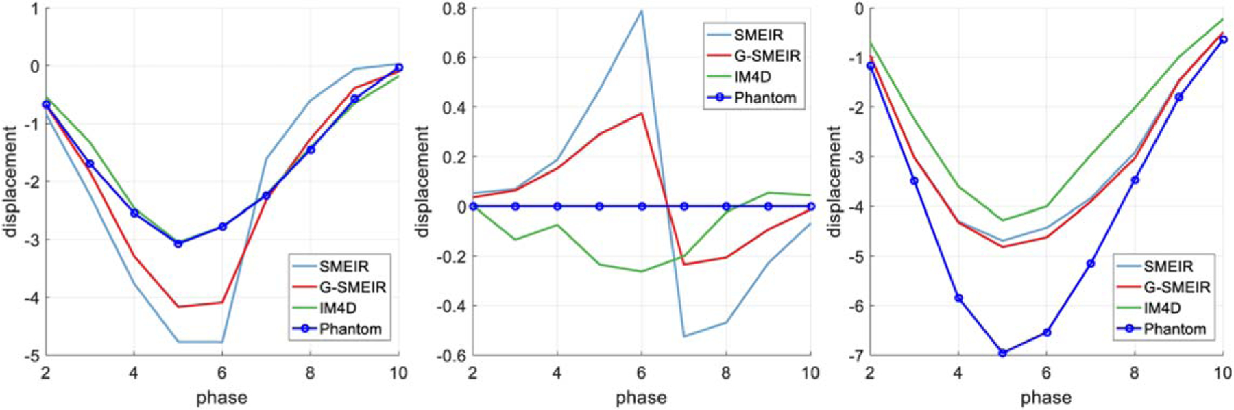
The maximum (‘MAX’) and mean deviations (in voxels) from the tumor phantom motion obtained from DVFs are listed in table 4. It can be seen that G-SMEIR usually achieves the smallest maximum and mean deviations compared to SMEIR and IM4D. It is also worth noting that although SMEIR has smaller maximum deviations than IM4D, its mean deviations are worse than IM4D. The overall improvement of G-SMEIR over SMEIR in terms of mean deviation is 42%~47% at different dose levels. The motion displacements of the tumor in Anterior-Posterior (A-P), Left-Right (L-R), and Superior-Inferior (S-I) at full dose are shown in figure 11, where the ordinate is the displacement (in voxels) and the abscissa is the number of phases. IM4D seems to recover the motion well in A-P and L-R directions, where the motion is small, but to become incapable of capturing the large motion in the S-I direction. In comparison, G-SMEIR not only recovers best the large motion in the S-I direction, but also improves the motion estimation in the other two directions over SMEIR. Note that the L-R motion was set as zero in the simulation. An abrupt transition around Phase 6 may be caused by residuals from the A-P motion for SMEIR and G-SMEIR. However, the amplitudes of these artificial L-R motions are small (less than ±1 voxel).

Table 4.

The maximum and mean deviations (voxel) from the phantom tumor motion for different reconstruction methods. (M, N) is for G-SMEIR.

		MAX	Mean
Full dose	IM4D	2.6785	0.5915
	SMEIR	2.2684	0.7220
	(2,11)	2.1405	0.5071
	(3,7)	2.0782	0.4354
	(4,5)	2.0771	0.4211
Half dose	IM4D	2.6642	0.5864
	SMEIR	2.3128	0.7316
	(2,11)	2.1553	0.5127
	(3,7)	2.0827	0.4449
	(4,5)	2.0730	0.4237
10% dose	IM4D	2.6679	0.5767
	SMEIR	2.3929	0.8079
	(2,11)	2.1784	0.5288
	(3,7)	2.0926	0.4480
	(4,5)	2.0778	0.4288

Figure 11.

Motion trajectories in different directions for different reconstruction methods. (From left to right: A-P, L-R, and S-I).

3.6. Patient results

The reconstructed patient images for two phases are shown in figure 12 (Phase 1) and figure 13 (Phase 7) (with HU range of [−1000 4434]), respectively. IM4D, SMEIR, and G-SMEIR show much better image quality than 3D TV, which suffers more noise and blocky artifacts due to the limited views for each phase. For the reference phase (figure 12, Phase 1), all three motion-compensated methods achieve a similar image quality, which is consistent with the findings in the phantom study. However, for Phase 7 in figure 13, G-SMEIR not only maintains the contents in the lunges better (yellow arrows), but also suffers less motion artifacts (red arrows) than IM4D and SMEIR. Some ringing artifacts (e.g. blue arrow in figure 12) in the sagittal view of MF-PMM methods can be seen due to non-optimized reconstruction parameters. Since 4D methods are much more time consuming than 3D TV, we were only able to tune parameters (ART step sizes: λ, λ_red, and TV minimization step sizes: γ, γ_red, see appendix for definitions) for patient data and used the other parameters from the simulation study for MF-PMM methods. When we lowered the TV regularization by reducing γ and γ_red, we observed the dominance of noise and streak artifacts for 3D TV images, while the images from MF-PMM methods (IM4D, SMEIR, and G-SMEIR) are similar. Also, the ringing artifacts in 4D MF-PMM methods are alleviated for smaller TV regularization. This demonstrates that the strong denoising and sparse data recovery of 4D reconstruction than 3D reconstruction. Note that these images were acquired for the patient positioning purpose of radiation therapy and the projection views for each phase was only 30, thus their quality is not as good as diagnostic CT images and serves as a comparative purpose here.

Figure 12.

Phase 1 images of the patient for different methods. From top to bottom: transverse, coronal, and sagittal; from left to right: 3D TV, IM4D, SMEIR, and G-SMEIR.

Figure 13.

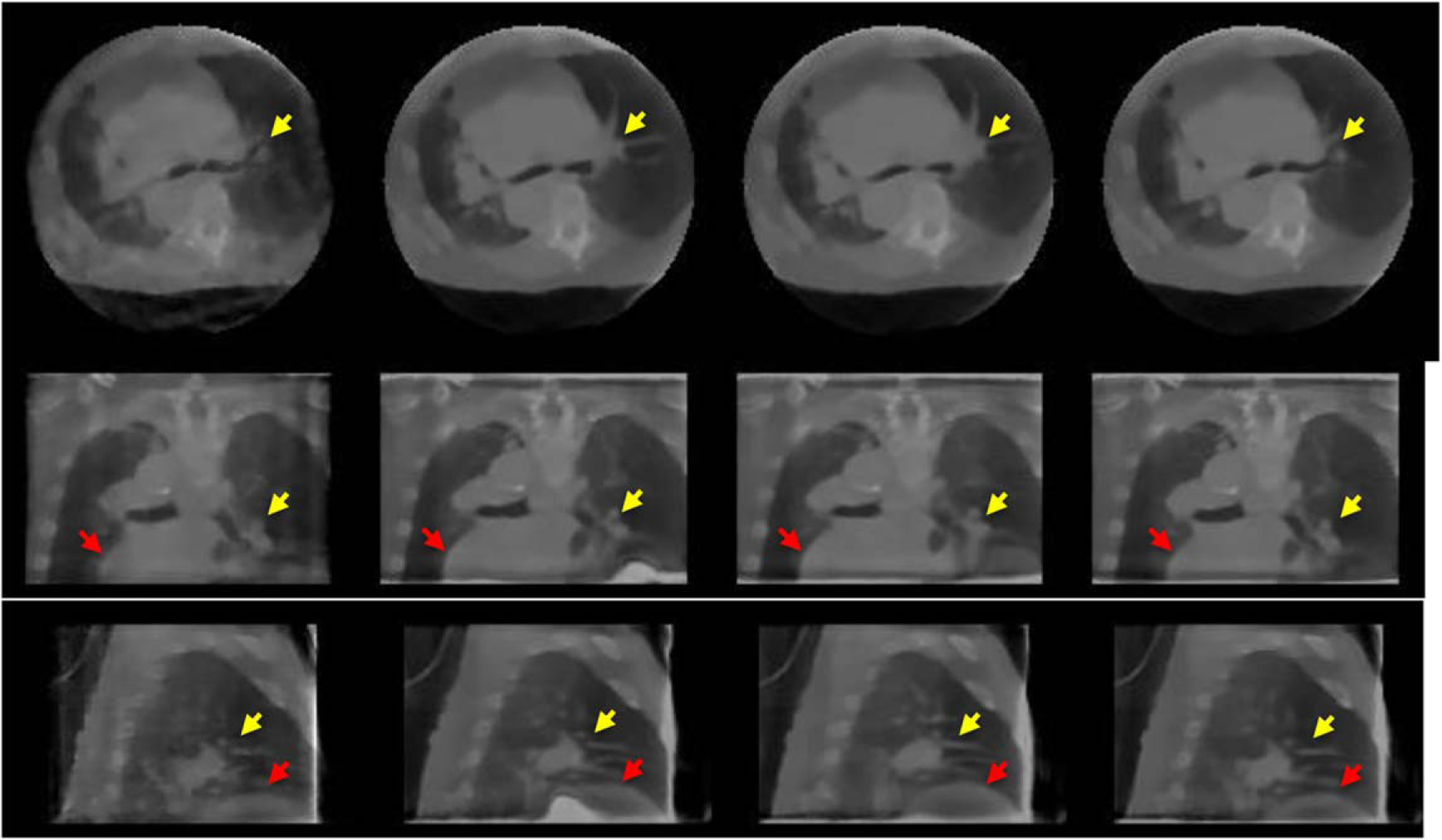
Phase 7 images of the patient for different methods. From top to bottom: transverse, coronal, and sagittal; from left to right: 3D TV, IM4D, SMEIR, and G-SMEIR.

4. Discussion and conclusions

We also tested other combinations for G-SMEIR, e.g. (M, N) = (6, 3) and (8, 2). The performance is similar to those reported in section 3. In general, we observed that the smaller M and the larger N leads to better RMSE, and the larger M and the smaller N leads to better SSIM. Although the improvement over RMSE and SSIM seems not to be substantial, G-SMEIR provides much better motion tracking of the tumor as indicated in table 4, where the mean motion tracking error is reduced by more than 40% compared to SMEIR. The flexibility of G-SMEIR may provide an effective tool to boost the 4D reconstruction performance of other imaging modalities, such as CT, PET, and SPECT.

For image domain motion estimation, we mainly focused on improving the speed through the faster convergence and GPU implementation. Although the Demons algorithm was used in this work, more sophisticated motion estimation algorithms can be used to further improve the DVFs, thus the final reconstruction. It seems that the projection domain motion estimation using a symmetric form leads to better reconstruction for SMEIR in terms of RMSE and SSIM, whereas the image domain motion estimation using Demons leads to better tumor motion tracking for IM4D. G-SMEIR takes advantage of both image domain and projection domain motion estimation to achieve the best performance in all quantitative metrics as well as the appearance of reconstruction images.

It is also worth noting that the motion-compensated reconstruction methods belonging to MF-PMM (IM4D, SMEIR, and G-SMEIR) hold great potential for dose reduction. When the imaging dose was reduced from 10⁵ photons/incident ray to 5 × 10⁴ photons/incident ray, the RMSE and SSIM values changed little. Only when the dose was reduced to 1 × 10⁴ photons/incident ray, a few percent decrease on RMSE was observed. The strong denoising and data compression capability of these methods are achieved by using both spatial (TV minimization) and temporal (motion-compensated joint reconstruction) correlations in phase images. The superior reconstruction quality can be seen from the patient images, where each phase has only 30 projection views. Among three motion compensated reconstruction methods, G-SMEIR reveals more anatomic details than IM4D and SMEIR, which further demonstrates the power of combining both image domain and projection domain motion estimation for better reconstruction of 4D images.

The flat-panel detector in the XCAT phantom study was larger than the conventional one used in CBCT in order to cover the whole-body projection. By doing this, we can avoid the truncation in the projection domain and focus on studying the behavior of different reconstruction methods under an idealized condition. In real patient data, the half-scan was used due to the size of the flat-panel detector. Nevertheless, the reconstruction performance ranking of different methods is consistent with findings in the simulation study.

In this work, G-SMEIR was run on the Maverick2 GPU server at Texas Advanced Computing Center (TACC). The image domain motion estimation ran on GPUs (NVidia P100 GPU), while the projection domain motion estimation ran on CPUs (Intel^® Xeon^® Platinum 8160 CPU). The reconstruction of each phase of P phases was implemented in parallel on one of the P CPU cores, providing P times saving on computation time. Both two domain motion estimations run parallel to reduce time consumption. It takes about 1,000 seconds to complete image domain motion estimation, 220 seconds to complete joint ART reconstruction, and 1,600 seconds to complete projection domain motion estimation. Note that since I/O operations of large DVF files are included in the calculation, the time reported for image domain estimation is much longer than the runtime of the MRD algorithm. The biggest computational bottleneck is the projection domain motion estimation, which includes the optimization of motion objective functions and multiple projection and warping operations. It is expected that GPU parallel computing can significantly reduce the runtime for this part similar to image domain motion estimation. The parallelization of projection/backprojections will further reduce the ART operations. Finally, a clever scheme of using DVFs is in need to avoid excessive I/O operations. In the future, we will investigate these possibilities to further lower the computation cost, which is essential for parameter tuning and selection of deformable registration models of G-SMEIR for better performance.

In summary we develop a G-SMEIR framework for MF-PMM to alleviate the local optimum trapping problem of 4D image reconstruction and accelerated the computational intense image domain motion estimation using GPU. The results using a 4D XCAT phantom and patient CBCT data demonstrate the superior reconstruction performance of G-SMEIR in a manageable time.

Appendix

The G-SMEIR pseudo-code is listed below along with SMEIR, TV minimization (Wang and Gu 2013) and the image domain Demons registration (Vercauteren et al 2009, Jin et al 2013b).

The parameters shown in the pseudo code were used to reconstruct images in this work, unless otherwise stated. Particularly, to balance the TV constraint and the data fidelity term, the numbers of ART and TV iterations were set as 20 and 5, respectively. The step size parameters, λ, λ_red, γ, γ_red, were 0.1, 1, 0.1, and 0.8 for the phantom data, and 0.1, 0.99, 0.3, and 0.9 for the patient data. These parameters were tuned using 3D TV for the best RMSE of phantom reconstruction and through visual inspection of patient reconstruction. In addition, G-SMEIR performance is influenced by M_Iteration and N_Iteration as shown in the results.

References

- Bai W and Brady M 2009. Regularized B-spline deformable registration for respiratory motion correction in PET images Phys. Med. Biol 54 2719. [DOI] [PubMed] [Google Scholar]
- Blume M, Martinez-Moller A, Keil A, Navab N and Rafecas M 2010. Joint reconstruction of image and motion in gated positron emission tomography IEEE Trans. Med. Imaging 29 1892–906 [DOI] [PubMed] [Google Scholar]
- Brehm M, Paysan P, Oelhafen M, Kunz P and Kachelrieß M 2012. Self-adapting cyclic registration for motion-compensated cone-beam CT in image-guided radiation therapy Med. Phys 39 7603–18 [DOI] [PubMed] [Google Scholar]
- Chun SY and Fessler JA 2009. Joint image reconstruction and nonrigid motion estimation with a simple penalty that encourages local invertibility Proc. SPIE 7258, Medical Imaging 2009 Physics of Medical Imaging 72580U [Google Scholar]
- Chun SY and Fessler JA 2012a. Noise properties of motion-compensated tomographic image reconstruction methods IEEE Trans. Med. Imaging 32 141–52 [DOI] [PMC free article] [PubMed] [Google Scholar]
- Chun SY and Fessler JA 2012b. Spatial resolution properties of motion-compensated tomographic image reconstruction methods IEEE Trans. Med. Imaging 31 1413–25 [DOI] [PMC free article] [PubMed] [Google Scholar]
- Dawant BM 2002. Non-rigid registration of medical images: purpose and methods, a short survey Proc. IEEE Int. Symp. on Biomedical Imaging (Piscataway, NJ) (IEEE) pp 465–8 [Google Scholar]
- Dawood M, Lang N, Jiang X and Schafers KP 2006. Lung motion correction on respiratory gated 3-D PET/CT images IEEE Trans. Med. Imaging 25 476–85 [DOI] [PubMed] [Google Scholar]
- Gravier E, Yang Y and Jin M 2007. Tomographic reconstruction of dynamic cardiac image sequences IEEE Trans. Image Process 16 932–42 [DOI] [PubMed] [Google Scholar]
- Gu X, Choi D, Men C, Pan H, Majumdar A and Jiang SB 2009. GPU-based ultra-fast dose calculation using a finite size pencil beam model Phys. Med. Biol 54 6287. [DOI] [PMC free article] [PubMed] [Google Scholar]
- Han G, Liang Z and You J 1999. A fast ray-tracing technique for TCT and ECT studies IEEE Nuclear Science Symp. and Medical Imaging Conf. 3 (Piscataway, NJ) (IEEE) 1515–8 [Google Scholar]
- Horn BK and Schunck BG 1981. Determining optical flow Artificial intelligence 17 185–203 [Google Scholar]
- Jacobson M and Fessler JA 2003. Joint estimation of image and deformation parameters in motion-corrected PET IEEE Nuclear Science Symp. and Medical Imaging Conference vol Series 5 (Piscataway, NJ) (IEEE) 3290–4 [Google Scholar]
- Jin M, Niu X, Qi W, Yang Y, Dey J, King MA, Dahlberg S and Wernick MN 2013a. 4D reconstruction for low-dose cardiac gated SPECT Med. Phys 40 022501. [DOI] [PMC free article] [PubMed] [Google Scholar]
- Jin M, Yang Y and King MA 2006. Reconstruction of dynamic gated cardiac SPECT Med. Phys 33 4384–94 [DOI] [PubMed] [Google Scholar]
- Jin M, Yang Y, Niu X, Marin T, Brankov JG, Feng B, Pretorius PH, King MA and Wernick MN 2009. A quantitative evaluation study of four-dimensional gated cardiac SPECT reconstruction Phys. Med. Biol 54 5643. [DOI] [PMC free article] [PubMed] [Google Scholar]
- Jin S, Li D, Wang H and Yin Y 2013b. Registration of PET and CT images based on multiresolution gradient of mutual information demons algorithm for positioning esophageal cancer patients Journal of applied clinical medical physics 14 50–61 [DOI] [PMC free article] [PubMed] [Google Scholar]
- Kalantari F, Li T, Jin M and Wang J 2016. Respiratory motion correction in 4D-PET by simultaneous motion estimation and image reconstruction (SMEIR) Phys. Med. Biol 61 5639–61 [DOI] [PMC free article] [PubMed] [Google Scholar]
- Klein G, Reutter B and Huesman R 1997. Non-rigid summing of gated PET via optical flow IEEE Trans. Nucl. Sci 44 1509–12 [Google Scholar]
- Kumar P, Das S, Park J, Badkul R, Hus S and Wang F 2012. Four-dimensional Cone Beam CT (4D-CBCT) Significantly Improves Localization of Lung Tumors in Comparison to x-Ray 6D Image Guidance in the Delivery of Stereotactic Body Radiation Therapy (SBRT) International Journal of Radiation Oncology, Biology, Physics 84 S743 [Google Scholar]
- Lamare F, Carbayo ML, Cresson T, Kontaxakis G, Santos A, Le Rest CC, Reader A and Visvikis D 2007. List-mode-based reconstruction for respiratory motion correction in PET using non-rigid body transformations Phys. Med. Biol 52 5187. [DOI] [PubMed] [Google Scholar]
- Li T, Thorndyke B, Schreibmann E, Yang Y and Xing L 2006. Model-based image reconstruction for four-dimensional PET Med. Phys 33 1288–98 [DOI] [PubMed] [Google Scholar]
- Mair BA, Gilland DR and Sun J 2006. Estimation of images and nonrigid deformations in gated emission CT IEEE Trans. Med. Imaging 25 1130–44 [DOI] [PubMed] [Google Scholar]
- Morton LM, Onel K, Curtis RE, Hungate EA and Armstrong GT 2014. The rising incidence of second cancers: patterns of occurrence and identification of risk factors for children and adults American Society of Clinical Oncology Educational Book 34 e57–67 [DOI] [PubMed] [Google Scholar]
- Mory C, Janssens G and Rit S 2016. Motion-aware temporal regularization for improved 4D cone-beam computed tomography Phys. Med. Biol 61 6856. [DOI] [PubMed] [Google Scholar]
- Nehmeh SA, Erdi YE, Ling CC, Rosenzweig KE, Schoder H, Larson SM, Macapinlac HA, Squire OD and Humm JL 2002. Effect of respiratory gating on quantifying PET images of lung cancer J. Nucl. Med 43 876–81 (https://jnm.snmjournals.org/content/43/7/876) [PubMed] [Google Scholar]
- Qiao F, Pan T, Clark JW Jr and Mawlawi OR 2006. A motion-incorporated reconstruction method for gated PET studies Phys. Med. Biol 51 3769. [DOI] [PubMed] [Google Scholar]
- Qin A, Gersten D, Liang J, Liu Q, Grill I, Guerrero T, Stevens C and Yan D 2018. A clinical 3D/4D CBCT-based treatment dose monitoring system J Appl Clin Med Phys 19 166–76 [DOI] [PMC free article] [PubMed] [Google Scholar]
- Ritchie CJ, Hsieh J, Gard MF, Godwin JD, Kim Y and Crawford CR 1994. Predictive respiratory gating: a new method to reduce motion artifacts on CT scans Radiology 190 847–52 [DOI] [PubMed] [Google Scholar]
- Segars WP, Sturgeon GS, Grimes J and Tsui BM 2010. 4D XCAT phantom for multimodality imaging research Med. Phys 37 4902–15 [DOI] [PMC free article] [PubMed] [Google Scholar]
- Shrestha D, Tsai M-Y, Qin N, Zhang Y, Jia X and Wang J 2019. Dosimetric evaluation of 4D-CBCT reconstructed by Simultaneous Motion Estimation and Image Reconstruction (SMEIR) for carbon ion therapy of lung cancer Med. Phys 46 4087–94 [DOI] [PMC free article] [PubMed] [Google Scholar]
- Sonke JJ, Zijp L, Remeijer P and van Herk M 2005. Respiratory correlated cone beam CT Med. Phys 32 1176–86 [DOI] [PubMed] [Google Scholar]
- Sweeney RA, Seubert B, Stark S, Homann V, Müller G, Flentje M and Guckenberger M 2012. Accuracy and inter-observer variability of 3D versus 4D cone-beam CT based image-guidance in SBRT for lung tumors Radiation Oncology 7 81. [DOI] [PMC free article] [PubMed] [Google Scholar]
- Taguchi K, Sun Z, Segars WP, Fishman EK, Tsui BM and Medical Imaging 2007. Image-domain motion compensated time resolved 4D cardiac CT Proc. SPIE Medical Imaging (Physics of Medical Imaging) ( 10.1117/12.709980) [DOI] [Google Scholar]
- Thirion J-P 1998. Image matching as a diffusion process: an analogy with Maxwell’s demons Med. Image Anal 2 243–60 [DOI] [PubMed] [Google Scholar]
- Van Stevendaal U, Von Berg J, Lorenz C and Grass M 2008. A motion-compensated scheme for helical cone-beam reconstruction in cardiac CT angiography Med. Phys 35 3239–51 [DOI] [PubMed] [Google Scholar]
- Vercauteren T, Pennec X, Perchant A and Ayache N 2009. Diffeomorphic demons: Efficient non-parametric image registration Neuroimage 45 S61–72 [DOI] [PubMed] [Google Scholar]
- Wang J and Gu X 2013. Simultaneous motion estimation and image reconstruction (SMEIR) for 4D cone-beam CT Med. Phys 40 101912. [DOI] [PubMed] [Google Scholar]
- Zhang H, Zeng D, Zhang H, Wang J, Liang Z and Ma J 2017. Applications of nonlocal means algorithm in low-dose X-ray CT image processing and reconstruction: A review Med. Phys 44 1168–85 [DOI] [PMC free article] [PubMed] [Google Scholar]
- Zhao C, Zhong Y, Duan X, Zhang Y, Huang X, Wang J and Jin M 2018. 4D cone-beam computed tomography (CBCT) using a moving blocker for simultaneous radiation dose reduction and scatter correction Phys. Med. Biol 63 115007. [DOI] [PMC free article] [PubMed] [Google Scholar]
- Zhao C, Zhong Y, Wang J and Jin M 2017. Modified simultaneous motion estimation and image reconstructioN (M-SMEIR) for 4D-CBCT IEEE 15th International Symposium on Biomedical Imaging 340–3 [Google Scholar]