A framework for constraining image SNR loss due to MR raw data compression

Abstract

Introduction

Computationally intensive image reconstruction algorithms can be used online during MRI exams by streaming data to remote high-performance computers. However, data acquisition rates often exceed the bandwidth of the available network resources creating a bottleneck. Data compression is, therefore, desired to ensure fast data transmission.

Methods

The added noise variance due to compression was determined through statistical analysis for two compression libraries (one custom and one generic) that were implemented in this framework. Limiting the compression error variance relative to the measured thermal noise allowed for image signal-to-noise ratio loss to be explicitly constrained.

Results

Achievable compression ratios are dependent on image SNR, user-defined SNR loss tolerance, and acquisition type. However, a 1% reduction in SNR yields approximately four to ninefold compression ratios across MRI acquisition strategies. For free-breathing cine data reconstructed in the cloud, the streaming bandwidth was reduced from 37 to 6.1 MB/s, alleviating the network transmission bottleneck.

Conclusion

Our framework enabled data compression for online reconstructions and allowed SNR loss to be constrained based on a user-defined SNR tolerance. This practical tool will enable real-time data streaming and greater than fourfold faster cloud upload times.

Introduction

Advanced image reconstruction algorithms have become ubiquitous in MRI research [1]. In many cases these reconstructions are implemented offline, due to the requirement for more computational power than is available on vendor reconstruction hardware [2, 3]. As a result, there is a growing need for practical tools that enable custom reconstructions to be performed online within the clinical environment, such that images can be reconstructed and return to the scanner host during the exam, rather than restricting custom algorithms to offline workflows.

Software platforms, such as the Gadgetron [3], that enable online custom reconstructions rely on streaming data across a network to external computers or cloud environments [4] during clinical exams. Sometimes the volume of data can exceed the network bandwidth, for example, a real-time Cartesian acquisition with 32 channels, 256 samples per readout, and 3-ms TR would require more than 21 MB/s of available bandwidth for data transfer to keep pace with acquisition. A spiral imaging sequence, that inherently has a higher acquisition duty cycle, will exceed 50 MB/s. Gigabit ethernet (125 MB/s) is increasingly common, but sufficiently high bandwidth may still not be practically achievable in the hospital environment, and many sites around the world still have limited network resources.

To alleviate any bottlenecks in fast image reconstruction caused by the transfer of data, networked reconstructions could significantly benefit from data compression for increased streaming capabilities. Data compression is common for storing and transmitting all varieties of digital multimedia (ex. MPEG-4 for audio/video) and is also becoming increasingly accepted for scientific computing [5, 6]. However, to date, the effect of data compression algorithms on MRI raw data (k-space) has not been investigated. Note that raw data here refer to the MR signal sampled at the receiver, before any reconstruction takes place. It is important to distinguish raw data compression from image compression, because reconstructed image data are small relative to the high-precision, multi-channel raw data, and do not require compression to transmit efficiently over a network.

Data compression comes in two forms, lossless and lossy. Lossless compression rates are modest, particularly of noisy, high-precision data, since lossless algorithms work by exploiting statistical redundancy. Lossy compression rates can be significantly higher. Lossy compression works by reducing the precision of the data (i.e. truncating the number of bits used to represent each value) resulting in irreversible losses. Losses to MR image quality are clinically unacceptable; however, since MR data are inherently noisy, reducing the precision does not necessarily reduce the fidelity of the data. For example, many of the bits in a 32-bit receiver value may have significance that is below the noise level. Thus, MR data are in fact well suited for lossy compression because, in the presence of noise, truncation will result in only a modest reduction in relative image signal-to-noise ratio (SNR). A small SNR penalty is unavoidable when using lossy data compression, but it is important that any losses are small and predictable.

The purpose of this study is to validate that the SNR loss can be explicitly constrained (e.g. 1% SNR loss) and assess achievable compression ratios at various SNR tolerance levels. In this work we describe, implement, and test a framework that enables the user to apply raw data compression with a tolerance level prescribed in terms of relative image SNR loss. The same framework is demonstrated using two different compression schemes: (1) a basic and MR-specific lossy compression strategy, referred to in this work as “NHLBI compression” and (2) an existing high-performance compression scheme (the open-source ZFP compression library [5]). It is not the goal of this work to introduce a new compression algorithm, but rather to show that the same statistical analysis can be performed for any algorithm to achieve SNR-constrained MRI raw data compression. Finally, we apply this data compression framework for cloud-based reconstruction of free-breathing continuous acquisition cardiac cine data.

Methods

Principles of lossy compression

Lossy compression schemes typically follow the same workflow:

1. Decorrelating the data using an orthogonal transform: this gets rid of any spikes or unexpected periodicity, resulting in a flat, smoothly varying signal. Lower dynamic range corresponds to higher compression rates for the same amount of losses.

2. The floating-point representation is converted to block float representations, where all the values are scaled to a common exponent. This step is lossless; the exponent bits can be stripped from each floating-point value, stored once in a header as an integer value, and then returned upon decompression with no loss in precision.

3. The block float values are converted to a compacted (unsigned) representation to prepare for truncation.

4. The truncation of least-significant bits: this step results in an irreversible loss in precision. The number of bits discarded depends on some user-defined input. In many compression algorithms, the user can specify either the precision that should be maintained after compression or the maximum compression error.

The decompression algorithm is a mirror of the compression algorithm. However, it needs to know the precision of the compacted data and the value of the common block float exponent. Therefore, these data are generally appended to the compacted data as a header.

NHLBI compression

To demonstrate the statistical analysis of compression on MRI raw data noise, we introduce an in-house lossy compression library, which follows a similar pipeline specifically simplified for MR raw data. The purpose of the NHLBI compression was not to compete with advanced lossy compression libraries, rather to achieve meaningful compression ratios while maintaining a compression workflow that was fast and easy to analyze within this framework.

NHLBI compression scheme: (1) scales the dataset by a common floating-point scale factor, (2) rounds the result to the nearest integer, and (3) truncates to the minimum precision required to represent the largest integer in the set.

Using this approach makes assessing compression error simple and intuitive. We define compression error as the difference between the original data and the compressed/decompressed data. The maximum error that can be made is half of the chosen scale factor (since the algorithm cannot make more than 0.5 error rounding to the nearest integer). The NHLBI compression scheme allows the maximum compression error (also known as the compression tolerance, ε) to be specified as an input.

A compression buffer contains a fixed-size header followed by a variable length compressed data bit stream. The compression ratio is defined as the size of the original data divided by the size of the compression buffer. The compression ratio is dependent on the precision needed to represent the largest integer in the data set after scaling and truncation. Hence, higher dynamic range signals result in lower compression at equivalent tolerance.

NHLBI compression does not use an explicit decorrelation transform, we instead employ a segmentation strategy that accomplishes a similar goal of reducing dynamic range. Rather than compressing an entire readout line into a single buffer, better compression results were achieved by dividing the data into multiple smaller segments containing smaller dynamic range (Fig. 1), exploiting the natural temporal smoothness of MR data. In addition, this approach requires less computational time than a decorrelation transform.

Fig. 1.

Schematic of a segmented raw data with the NHLBI compression. Each channel is divided into five segments to reduce the dynamic range of many of the segments. In this Cartesian example, the outer four segments can be compressed the most. A fixed-size header is attached to all individual compression buffers, which contains the parameters for decompression

The compression ratio of each segment will vary based on the dynamic range exhibited in each segment, even though the compression tolerance is set to the same value. Data segments from the outer parts of k-space that contain mostly noise can be compressed at much higher rates than if the whole acquisition was put in the same buffer. The optimal segment size varies depending on the data. However, it was empirically observed that five segments per channel yielded good compression rates for a variety of acquisition types (i.e. Cartesian, spiral, and radial).

NHLBI compression error statistics

Error introduced by compression is comparable to adding noise to the signal and will manifest as a predictable decrease in SNR. Considering that the noise in the acquisition and the noise due to compression are uncorrelated, the resulting variance of the total noise can be expressed as the sum of the variances:

$${\sigma }^2={\sigma }_{\text{n}}^2+{\sigma }_{\text{c}}^2,$$ (1)

where σ_n is the standard deviation of the noise in the acquired MR signal and σ_c is the standard deviation of the error contributed by the compression. Assuming the compression tolerance (ε) is small relative to the data magnitude, the errors will be randomly distributed uniformly between ± ε and centered at zero. The variance of a random uniform distribution is well defined as ${\sigma }^2=\frac{{(b-a)}^2}{12}$, where a and b are the lower and upper limits. Thus, the variance added by NHLBI compression can be expressed by

$${\sigma }_{\text{c}}^2=\frac{{(2\epsilon )}^2}{12}.$$ (2)

As the Fourier transform is a linear operator, the noise variance in the image domain is the same as the noise variance in the acquisition data. Additionally, the image noise will always be Gaussian regardless of the added noise distribution as the central limit theorem states that the sum of random independent variables results in a Gaussian distribution. We can compute SNR of the compressed data image relative to the original image as the ratio of the original signal noise to the decompressed signal noise. Here, we define T, as the SNR tolerance determined by the relative SNR loss:

$$T=1-\mathrm{rel}.\mathrm{SNR}=1-\frac{{\sigma }_{\text{n}}}{\sqrt{{\sigma }_{\text{n}}^2+{\sigma }_{\text{c}}^2}}.$$ (3)

Combining Eqs. 2 and 3, and solving for the compression tolerance (ε) yields

$$\epsilon =\sqrt{3}{\sigma }_{\text{n}}\sqrt{\frac{1}{{(1-T)}^2}-1}.$$ (4)

The key to our proposed framework is to set the tolerance based on a user-defined maximal SNR loss (T). Then the compression tolerance (ε) can be used as input parameter to the NHLBI and ZFP compression, to constrain the SNR loss using the noise standard deviation from the coil calibrations.

ZFP compression

The open-source ZFP compression scheme provides general purpose compression for floating-point arrays [5] (e.g. visualization, quantitative data analysis, and numerical simulation). This algorithm was tested to illustrate that the compression framework was applied generically to constrain SNR loss for any algorithm.

The high-level operation is similar to the generic pipeline described earlier. The floating-point data are aligned to a common exponent, then converted to fixed point, transformed for decorrelation, then reordered, and finally encoded.

Using the ZFP algorithm, we compress each one-dimensional channel readout separately and create multidimensionality by defining each per channel readout as two-dimensional real-valued array of size N/2 × 4, where N is the number of complex samples in a readout. We used “fixed tolerance mode”, where the maximum error can be defined.

Unlike the NHLBI compression, the ZFP error distribution is not uniform (it appears Gaussian-like) and the linear relationship between σ_c and ε was determined empirically by compressing Gaussian noise for a range of tolerance values. The ZFP tolerance is always a power of $2\left({\epsilon }_{\text{zfp}}=2^{\wedge }\text{floor}(\log 2(\epsilon ))\right)$, since the ZFP algorithm aligns each value to a common exponent of base 2. Using the empirically determined linear relationship between ε_ZFP and σ_c, the noise from ZFP compression can be described by

$${\sigma }_{\text{c}}^2=0.0074{\epsilon }_{\text{ZFP}}^2$$ (5)

Equations 3 and 5 can be combined to determine how to set the ZFP compression tolerance to constrain SNR tolerance.

$$\epsilon =\frac{1}{0.0863}{\sigma }_{\text{n}}\sqrt{\frac{1}{{(1-T)}^2}-1}.$$ (6)

However, ε in Eq. 6 and ε_zfp in Eq. 5 are only equal when ε is a power of 2. Therefore, the actual SNR loss will rarely be equal to the SNR tolerance but constrained under it.

Noise measurement and prewhitening

Constraining SNR loss in MR data compression requires that the standard deviation of the noise in the signal (σ_n) is known prior to the determination of the compression tolerance, ε. This noise was computed from a prescan in which the scanner receiver channels are sampled without the application of an excitation pulse, thus only sampling noise. For a multi-channel receive array, this measurement can be used to determine the noise covariance matrix, where the diagonal is the noise variance in each channel [7].

Often, this noise prescan measurement is used in image reconstructions for noise prewhitening [8]. Prewhitening creates a set of virtual channels from the data where the noise in each channel is uncorrelated and has variance equal to one. This is an important tool for optimizing SNR for MRI data acquired with phased array coils where noise levels may vary from coil element to coil element and noise in neighboring coil elements may be correlated. It is also a necessary step to reconstructing images scaled in SNR units [9]. Compression adds noise to the acquisition before the prewhitening step. Therefore, to maintain SNR units when using compression, we must modify the noise covariance matrix to account for the added compression noise (σ_c) on the diagonal elements.

Online remote reconstruction pipeline

The constrained lossy compression framework was implemented and validated in the Gadgetron reconstruction platform to enable data streaming to external computational resources for reconstruction. The code is available on the Gadgtron github repository (https://github.com/gadgetron/gadgetron).

MR experiments were performed on a 1.5T system (Aera, Siemens, Erlangen, Germany), as illustrated in Fig. 2. A custom Siemens reconstruction program (Image Calculation Environment, Siemens, Princeton, NJ) was used to interface between the scanner and the remote resources running the Gadgetron. This program was modified for data compression. Compressed data are streamed to the Gadgetron for reconstruction using ISMRMRD format [10]. The compression tolerance (Eqs. 4, 6) was determined from the pre-computed noise covariance matrix and the user-defined SNR tolerance which is an editable parameter on the MR host machine.

Fig. 2.

Flowchart illustrating the process for online remote reconstruction that was used. The orange boxes represent the compression/decompression stages that were added to the existing remote online reconstruction pipeline

Gadgetron has a standalone client application which emulates the transmission of data from a MR scanner. This was used to initially test simulations and phantom data compression and passing it to a Gadgetron reconstruction process.

The decompression was done on the reconstruction side. An ISMRMRD acquisition header contains flags to mark data as being compressed. There are separate flags for the NHLBI and ZFP compression schemes to distinguish between the two. Early in the reconstruction pipeline, the data are decompressed according to a header flag and passed downstream. Additional noise scaling is added to the prewhitening. Following this, the data are processed and reconstructed the same as any other MR data.

Experimental methods

The ability to constrain the SNR loss was validated through reconstructing simulated data. An eight-channel Cartesian simulated k-space dataset was generated from a noise-free Shepp–Logan image and an artificial coil sensitivity profile. Random Gaussian noise was added to 200 copies of this dataset to simulate repeated measurements for the determination of SNR. The amount of added noise was varied to produce multiple datasets with a range of SNR levels.

Phantom studies using a homogenous cylindrical phantom assessed noise and SNR for various acquisition types (Cartesian, EPI, spiral, and radial) and flip angles with compression. These data were also reconstructed offline using the standalone client application to perform compression. Imaging sequences used 128 × 128 pixel matrix with a 300 × 300 cm² FOV. The Cartesian sequence was run with flip angles varying from 2 to 25°. The spiral (eight shot) and radial sequences (200 lines per frame) were run with 2° and 10° flip angles. The single-shot EPI sequence used flip angles of 45° and 90°. Each imaging sequence had 200 dynamics for calculating SNR using the method of repeated measurements [11].

As an intended use case example, we tested the proposed framework on a free-breathing, continuous acquisition, Cartesian cardiac cine sequence [12] acquired in vivo over the left ventricular volume. These data were acquired in a healthy volunteer with written informed consent and local institutional review board approval. Commonly, data acquired using this sequence is reconstructed online using cloud nodes to parallelize the computationally intensive reconstruction along the slice dimension [4, 13]. Data were acquired continuously for 12 s per slice. The average data acquisition rate was approximately 37 MB/s, which would exceed the bandwidth of a fast ethernet network. Nine slices were acquired, resulting in a total data size of approximately 4 GB (typical data size will vary with acquisition parameters). These data were compressed using our proposed framework with a 1% SNR tolerance and compared to a reconstruction with no data compression, performed using the same data set retrospectively.

Results

Simulated data

The resultant effect of the compression framework on noisy simulated data can be visualized in Fig. 3. SNR changes from the original image can be observed though the relative loss maps which confirm that the SNR changes are bounded by the prescribed tolerance and that noise is added uniformly to the reconstructed image. This is displayed more clearly in Fig. 4 where the observed mean relative loss over the signal-containing portion of the image is plotted at various tolerance levels from 0 to 10%. For simulated data, where channel noise levels are equal and ideally uncorrelated, NHBLI compression allows the SNR loss to be specified exactly.

Fig. 3.

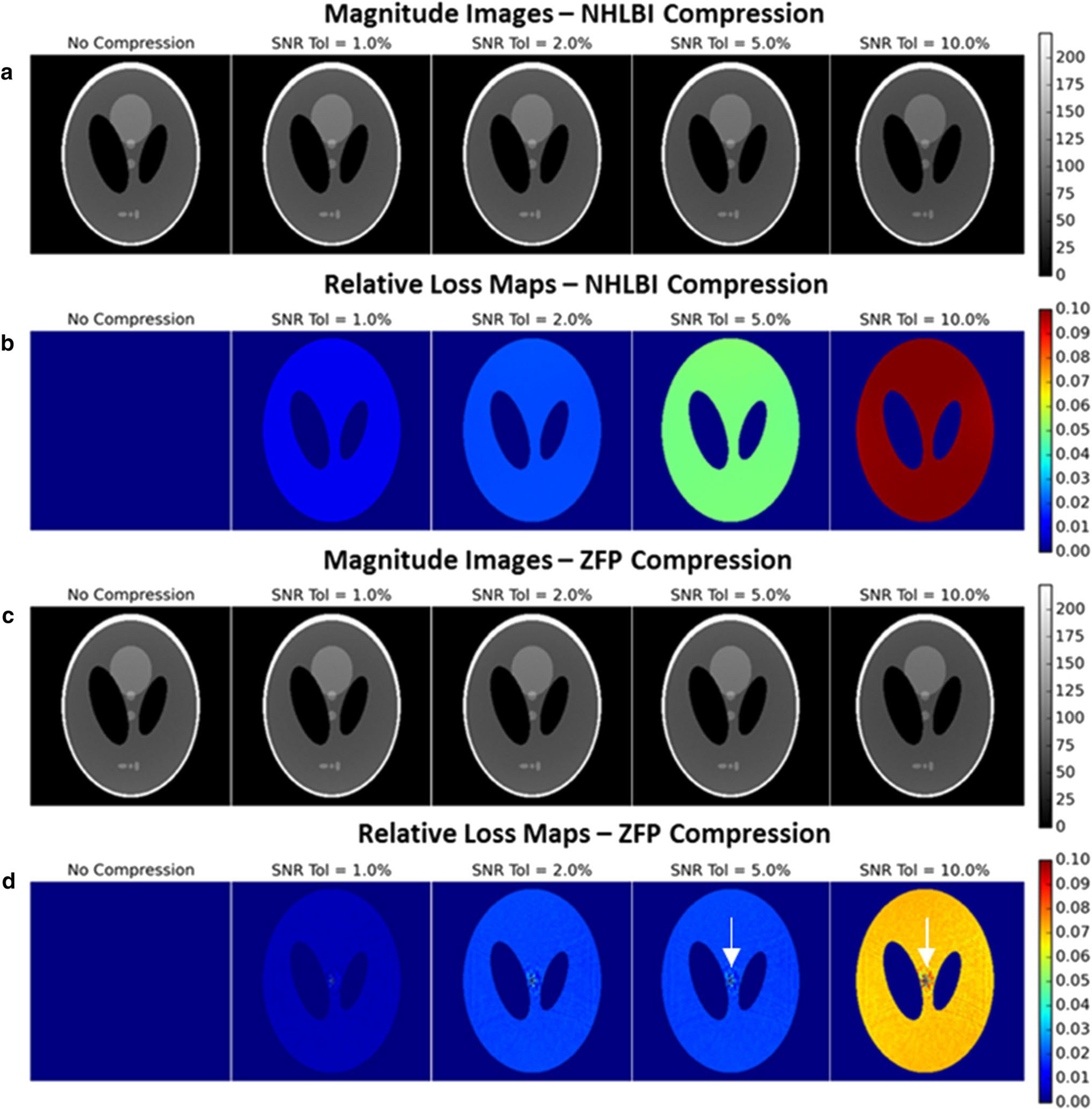
Reconstructed images using the simulated data with a mean SNR of 111 (a, c) with corresponding relative loss maps (b, d). The images are scaled to SNR units, thus SNR reduction results in a decrease in signal intensity relative to the phantom image reconstructed with no compression. The relative loss maps show that the relative loss is the same in all signal-containing regions (under the condition of ideally decoupled channel noise). A very small sinc-like compression artifact is noticeable in the ZFP relative loss maps (white arrows)

Fig. 4.

Measured relative SNR loss vs prescribed SNR tolerance for NHLBI (a) and ZFP compression (b) using simulated data at various SNR levels

The relative SNR loss using ZFP compression, however, does not follow a 1:1 relationship with the specified tolerance, instead the compression levels move in discrete jumps. This is expected for the ZFP algorithm because the compression tolerance (as defined in Eq. 6) is always rounded down to the nearest power of 2 and thus the SNR loss is held constant until the compression tolerance passes a certain threshold. The SNR loss is bounded by the specified SNR tolerance on the upper bound and $\frac{1}{4}$× SNR tolerance on the lower bound.

Simulations using a 0.5–10% tolerance over a SNR range from 46 to 624 yielded compression ratios from 3 to 7.5 (Fig. 5a). Analyzing the compression ratio versus the relative SNR loss shows that most of the compression occurs when the losses are constrained under 1%, which can yield compression ratios of 3–5.5.

Fig. 5.

a Compression ratios compared to relative SNR loss for simulated data. Lower SNR datasets can be compressed at higher ratios with equivalent losses. b Compression ratios with a fixed 1% SNR tolerance as a function of base SNR using simulated data

Figure 5b shows that compression ratio decreases with higher image SNR. The broad dynamic range of high-SNR signal requires more bits to encode and, therefore, have lower compression ratios.

Phantom studies

Phantom experiments representative of a clinical 1.5T MRI environment demonstrate that the SNR loss is not perfectly uniform over the entire image (Fig. 6), in contrast with the simulated data experiments. This is due to the small level of noise cross-correlation that exists amongst channels in realistic receive arrays and is further explained in the discussion. This effect can lead to the actual relative SNR loss to exceed the constrained tolerance, but by a marginal amount, particularly at SNR tolerance levels under 2% (Fig. 7). For example, relative SNR loss for NHLBI at 2% tolerance varied from 1.9 to 2.2%. With the ZFP algorithm, the same step-like pattern exists although it gets smoothed out by the differences in channel noise since not all jumps in discrete compression tolerance occur at the same increment in SNR tolerance. As with the simulated data, the ZFP SNR loss is bounded by the SNR tolerance and a quarter of the SNR tolerance.

Fig. 6.

Reconstructed images from a Cartesian GRE sequence with a mean SNR of 79 (a, c) with corresponding relative loss maps (b, d). The images are scaled to SNR units. The relative loss maps show that the loss is non-homogenous when channel noise is coupled, but the average SNR loss remains approximately bounded by the prescribed tolerance

Fig. 7.

Results from MR phantom experiments using a homogenous cylindrical phantom and a 32-channel array at 1.5T. Data were acquired with Cartesian, EPI, spiral and radial sampling and a normal range of SNR values achieved by changing the flip angle. User-specified SNR tolerance was stepped from 0.5% to 10% in increments of 0.5%. Validating the SNR tolerance of the framework using phantom data. NHLBI compression may exceed the SNR tolerance by a small margin (see “Discussion”)

Compression ratios using phantom data varied from approximately four to tenfold using a 0.5–10% SNR tolerance (Fig. 8). When constrained under 1% SNR loss, the compression ratios ranged from about 4.5–6.5 with ZFP and 5.5–6.5 with NHLBI in normal clinical SNR ranges. The acquisition type and SNR have an impact on the compression ratio since they influence the dynamic range of the readouts. Cartesian readout lines far from the central phase-encoding line contain very low signal relative to the noise level, therefore, making them highly compressible. Even though spiral readouts sample the center of k-space with every readout, the segmentation strategy in the NHLBI method significantly reduces dynamic range in each compressed segment. The ZFP algorithm uses a spread-spectrum decorrelation transform, resulting in higher compression rates for spiral acquisitions. A radial acquisition strategy also samples the center of k-space with each readout; however, since the length of the readouts are much shorter than with spiral, the segment size is shorter, and the number of compression buffer headers reduces the compression ratio. Overall, the influence of acquisition type is relatively minor compared to the influence of SNR on the compression ratio.

Fig. 8.

Measured relative SNR is plotted against compression ratios for different acquisition strategies

EPI and spiral scans have high sampling efficiency and are thus more likely to require compression for real-time streaming. The real-time, eight-interleave spiral acquired with 36 receive channels had a data acquisition rate of 56.5 MB/s. Using the NHLBI compression with a 1% SNR tolerance reduced the compressed data streaming rate to 10.3 MB/s for the higher SNR case (SNR = 112) and 8.7 MB/s for the lower SNR case (SNR = 26).

In vivo

A free-breathing continuous acquisition cardiac cine was reconstructed using the NHLBI compression scheme with a 1% SNR tolerance. Reconstructed images with and without compression are shown in Fig. 9. The SNR cannot be precisely measured from a single measurement; however, the SNR-scaled reconstruction yields a close estimate in high-SNR parts of the image. The measured pixel-wise relative loss was 0–3% in areas with appreciable signal and very close to 1% on average. A compression ratio of 6.08 was achieved for this application, reducing the required streaming bandwidth from 37 MB/s to approximately 6.1 MB/s for sending raw data to the cloud for reconstruction (reduction of 4 GB to 660 MB in total data size). To assess the effects of 1% SNR tolerance compression on clinical endpoints, we used Argus software (Siemens) to calculate the left ventricle (LV) end-systolic and end-diastolic volumes on the same dataset with and without compression. The mean difference in LV ejection fraction was 0.4% with a 3% standard deviation over three healthy subjects, which is within the intra-observer variability of these measurements [14], indicating no bias due to compression.

Fig. 9.

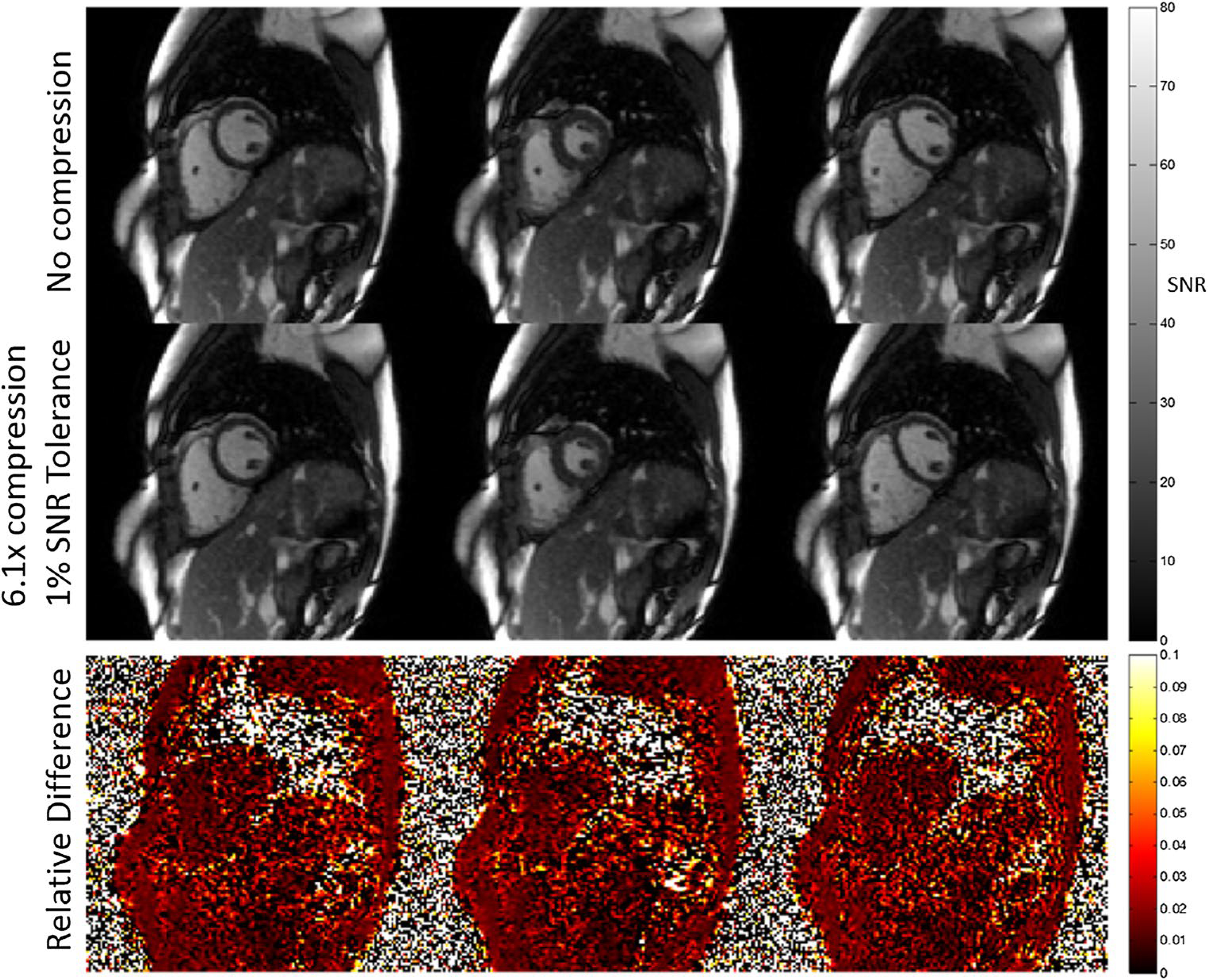
Example of real-time cardiac cine at three phases in a mid-ventricular, short-axis slice with and without a prescribed 1% SNR loss due to NHLBI compression. To facilitate online reconstruction of 30 cardiac phases with motion-correction, from 12 s of data per slice through the short axis, the data were compressed to a compression ratio of 6.1, and then transmitted to a remote workstation. The data were reconstructed retrospectively using the same pipeline without compression for comparison. The relative difference in the SNR-scaled reconstructions shows a small noise increase when compression is used (approximately 1% on average over high-SNR areas)

Discussion

This research demonstrates a framework to implement compression of MRI raw data, designed such that the signal-to-noise loss in the image is constrained to the user’s prescription. The framework leverages the understanding and calibration for noise within MRI systems, and applies a simple lossy compression approach to significantly reduce the required data size. This process can facilitate accelerated clinical workflows through utility of remote resources and has potential for use within open-source and collaborative environments. This method is essential for streaming large data sets over a slow network connection for online image reconstruction or dramatically reduce the time to upload data to the cloud.

The key to MR data compression is to constrain the losses to an acceptable threshold based on the noise level. Compression introduces random errors that are equivalent to adding noise to the signal. SNR loss in the image domain can be constrained based on a knowledge of the acquisition and compression noise. We expect that a 1% SNR loss will be tolerable in most clinical MRI settings and, furthermore, accepting losses beyond 1% does not provide a sufficiently attractive gain in compression ratio. As ‘day-to-day’ factors including coil position, coil loading, and parallel imaging can easily change the SNR by greater than 1%, we believe a SNR loss of 1% will not be obstructive. Our phantom study shows that one could expect a compression ratio of greater than 4.5 using a 1% SNR tolerance level based on realistic MRI data. The simulated data study, where each channel has the same noise level, represents the case where compression ratios will be the lowest since image noise with prewhitening is closely associated with the least noisy channel and the nosiest channels will be have high compression. In that regime, we can observe that the minimum compression ratio for SNR levels under 300 at 1% SNR tolerance is around 3.5 with ZFP and 4 with NHLBI.

A non-uniform SNR loss was observed in the acquired data, though not in the simulated data. Noise prewhitening allows us to display the images in SNR units. However, adding compression noise to the diagonal of the noise covariance matrix affects the sensitivity profiles of the virtual coils computed from prewhitening. In that sense, we can think of compression as effectively changing the physical noise properties of the receive coil. For example, compression with a 1% SNR tolerance will increase the noise on every channel by 1%, but will not have any effect on the correlated noise (off-diagonal elements of the noise covariance matrix). The net effect is an average SNR loss close to the prescribed level, but the relative loss map will be non-uniform due to the slight change in virtual channel sensitivities. This effect is not seen when the coil elements are completely decoupled, as in the simulated data. Despite this, the non-uniform SNR loss is not apparent in the images.

The NHBLI algorithm was implemented in this work as a tool to illustrate the statistical basis of the framework. It has the benefit of being intuitive to someone with little introduction into data compression and error distribution is the same as a random uniform distribution which makes the compression noise variance easy to predict. The SNR loss can be prescribed closely by the SNR tolerance, in contrast to block float-based compression, such as ZFP. Therefore, although simple, it is well suited for this application by design and results show that it can achieve more than adequate compression ratios. However, the central concepts of the proposed framework are compatible with any compression algorithm, thus was the motivation for including the ZFP compression scheme in this study.

In incorporating ZFP compression, we demonstrate the statistical analysis necessary to use a generic compression scheme in the proposed framework. While it is not our intention to compare the two compression schemes, the observed differences provide insight into important concepts. One of the major differences between the two compression schemes implemented is the use of an explicit decorrelation transform in ZFP and the lack of one in NHLBI. The segmentation strategy used in the NHLBI method exploits the fact that the general overall shape of the acquired MR signal is known [15]. Essentially, segmenting serves the same purpose as a decorrelation transform, which explains why the NHLBI compression implementation can achieve similar (and often higher) compression ratios relative to the ZFP method. However, ZFP’s decorrelation transform provides a clear benefit for achieving higher compression ratios in the case of spiral data, where segmenting does not decorrelate the data optimally. It is important to note that ZFP is designed to work best on multi-dimensional datasets where correlation exists along more than one dimension. Instead, in this framework, the performance of ZFP is limited by compressing each channel readout line (1D data) into a different compression buffer. Significantly higher compression rates are possible with ZFP by compressing all the channels together, given that correlation exists amongst channels. However, in this framework, it is necessary that every channel is constrained based on its own unique noise variance. An alternative would be to compress all channels to the same compression tolerance, using either the mean or the RMS noise variance of all the channels. This would allow much higher compression ratios using the ZFP algorithm but will not constrain the SNR loss in every individual channel image. Another potential disadvantage of the ZFP compression scheme for MR data is that it introduces a small artifact in the image domain which is noticeable when looking at the relative loss maps. The way the bit truncation is implemented introduces a small bias. The effect of a constant bias in the k-space data is an artifact that looks like a delta function in the image domain. This artifact is minor relative to the SNR tolerance (which is only a small percentage of the actual SNR) and only affects a few pixels. Such implementation considerations may be required for generic ‘black-box’ compression algorithms.

In addition to real-time streaming, compression could be beneficial in other areas, such as cloud computing and storage. Cloud reconstructions are used to accelerate computationally intensive reconstruction jobs. By reducing the data size, the data upload time will be reduced accordingly. Similarly, with the ubiquity of big data initiatives, one can imagine that compression could be very useful for data storage. It is becoming more common for people to save uncompressed raw MR datasets for future use. For example, machine learning-based image reconstruction programs need to be trained on large data set of MR raw data. The ability to reduce the data size with negligible decrease in data fidelity could have significant effects on storage costs and data transfer times. Recently, it has been shown that neural network-based MRI reconstruction can offer near real-time reconstruction using simple graphical processing units (GPUs) [16–18]. While this may alleviate some of the computational load of complex reconstruction jobs, it is yet to be seen whether such technologies will be incorporated into vendor-provided systems. Since machine learning reconstruction and processing algorithms often require a GPU-enabled computer and custom software, data streaming over a network connection to external computing resources may be important to make these techniques adaptable for clinical deployment. Therefore, raw MR data compression suggested here may also be valuable for future machine learning implementations.

Conclusion

As advanced reconstruction algorithms are brought to the clinical environment, we rely on the network transmission of raw MRI data to exploit computational resources and cloud computing. Connection bandwidth is a practical problem limiting real-time remote reconstructions which can be aided by lossy compression. Compression can also have a major impact on the time it takes to upload data to a cloud resource.

We have proposed and implemented a method for constraining relative SNR loss when compacting the size of MR raw data. The results show that significant compression is possible with relatively little losses. Accepting a very small, 1% SNR loss will yield compression rates that are more than adequate for most potential applications.

References

- 1.Yang AC, Kretzler M, Sudarski S, Gulani V, Seiberlich N (2016) Sparse reconstruction techniques in magnetic resonance imaging: methods, applications, and challenges to clinical adoption. Invest Radiol 51(6):349–364 [DOI] [PMC free article] [PubMed] [Google Scholar]
- 2.Uecker M, Lai P, Murphy MJ, Virtue P, Elad M, Pauly JM, Vasanawala SS, Lustig M (2014) ESPIRiT—an eigenvalue approach to autocalibrating parallel MRI: where SENSE meets GRAPPA. Magn Reson Med 71(3):990–1001 [DOI] [PMC free article] [PubMed] [Google Scholar]
- 3.Hansen MS, Sorensen TS (2013) Gadgetron: an open source framework for medical image reconstruction. Magn Reson Med 69(6):1768–1776 [DOI] [PubMed] [Google Scholar]
- 4.Xue H, Inati S, Sorensen TS, Kellman P, Hansen MS (2015) Distributed MRI reconstruction using Gadgetron-based cloud computing. Magn Reson Med 73(3):1015–1025 [DOI] [PMC free article] [PubMed] [Google Scholar]
- 5.Lindstrom P (2014) Fixed-rate compressed floating-point arrays. IEEE Trans Vis Comput Gr 20(12):2674–2683 [DOI] [PubMed] [Google Scholar]
- 6.Hübbe N, Wegener A, Kunkel JM, Ling Y, Ludwig T (2013) Evaluating lossy compression on climate data. In: Proceedings—supercomputing—28th international supercomputing conference, ISC 2013, Leipzig, Germany, pp 343–356 [Google Scholar]
- 7.Hansen MS, Kellman P (2015) Image reconstruction: an overview for clinicians. J Magn Reson Imaging 41(3):573–585 [DOI] [PMC free article] [PubMed] [Google Scholar]
- 8.Pruessmann KP, Weiger M, Börnert P, Boesiger P (2001) Advances in sensitivity encoding with arbitrary k-space trajectories. Magn Reson Med 46(4):638–651 [DOI] [PubMed] [Google Scholar]
- 9.Kellman P, McVeigh ER (2005) Image reconstruction in SNR units: a general method for SNR measurement. Magn Reson Med 54(6):1439–1447 [DOI] [PMC free article] [PubMed] [Google Scholar]
- 10.Inati SJ, Naegele JD, Zwart NR, Roopchansingh V, Lizak MJ, Hansen DC, Atkinson D, Kellman P, Xue H, Campbell-Washburn AE, Sørensen TS (2017) ISMRM Raw data format: a proposed standard for MRI raw datasets. Magn Reson Med 77(1):411–421 [DOI] [PMC free article] [PubMed] [Google Scholar]
- 11.Constantinides CD, Atalar E, McVeigh ER (1997) Signal-to-noise measurements in magnitude images from NMR phased arrays. Magn Reson Med 38(5):852–857 [DOI] [PMC free article] [PubMed] [Google Scholar]
- 12.Xue H, Kellman P, LaRocca G, Arai AE, Hansen MS (2013) High spatial and temporal resolution retrospective cine cardiovascular magnetic resonance from shortened free breathing real-time acquisitions. J Cardiovasc Magn Reson 15(1):102. [DOI] [PMC free article] [PubMed] [Google Scholar]
- 13.Cross R, Olivieri L, O’Brien K, Kellman P, Xue H, Hansen M (2016) Improved workflow for quantification of left ventricular volumes and mass using free-breathing motion corrected cine imaging. J Cardiovasc Magn Reson 18:10. [DOI] [PMC free article] [PubMed] [Google Scholar]
- 14.Yilmaz P, Wallexan K, Aben J, Moelker A (2018) Evaluation of a semi-automatic right ventricle segmentation method on short-axis MR images. J Digit Imaging 31:670–679 [DOI] [PMC free article] [PubMed] [Google Scholar]
- 15.Fuderer M (1988) The information content of MR images. IEEE Trans Med Imaging 7(4):368–380 [DOI] [PubMed] [Google Scholar]
- 16.Zhu B, Liu J, Cauley S, Rosen B, Rosen M (2018) Image reconstruction by domain-transform manifold learning. Nature 555:487–492 [DOI] [PubMed] [Google Scholar]
- 17.Wang G, Ye JC, Mueller K, Fessler J (2018) Image reconstruction is a new frontier of machine learning. IEEE Trans Med Imaging 37(6):1289–10296 [DOI] [PubMed] [Google Scholar]
- 18.Hammernik K, Klatzer T, Kobler E, Recht MP, Sodickson DK, Pock T, Knoll F (2018) Learning a variational network for reconstruction of accelerated MRI data. Magn Reson Med 79(6):3055–3071 [DOI] [PMC free article] [PubMed] [Google Scholar]