UMAP as Dimensionality Reduction Tool for Molecular Dynamics Simulations of Biomacromolecules: A Comparison Study

Abstract

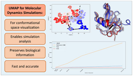
Proteins are the molecular machines of life. The multitude of possible conformations that proteins can adopt determines their free energy landscapes. However, the inherently high dimensionality of a protein free energy landscape poses a challenge to deciphering how proteins perform their functions. For this reason, dimensionality reduction is an active field of research for molecular biologists. The Uniform Manifold Approximation and Projection (UMAP) is a dimensionality reduction method based on a fuzzy topological analysis of data. In the present study, the performance of UMAP is compared to other popular dimensionality reduction methods such as t-Distributed Stochastic Neighbor Embedding (t-SNE), Principal Component Analysis (PCA), and time-structure Independent Components Analysis (tICA) in context of analyzing molecular dynamics simulations of the circadian clock protein Vivid. A good dimensionality reduction method should accurately represent the data structure on the projected components. The comparison of the raw high-dimensional data with the projections obtained using different dimensionality reduction methods based on various metrics, showed that UMAP has superior performance when compared with linear reduction methods (PCA and tICA), and has competitive performance and scalable computational cost.

Graphical Abstract

1. Introduction

Proteins are molecular engines present in all lifeforms on earth. Protein structures have been described hierarchically as protein primary, secondary, and tertiary structures. Main protein functional information is expected to be derived from this structural information. ^1–4 However, protein molecules are in constant dynamics, which also is a key factor in the regulation of the protein functions. ⁵

Molecular dynamics (MD) simulations provide dynamical information of protein conformations in order to map the protein conformational space, and thus rationalize protein function. ^6–8 The sampling of the protein conformations collected during the simulations compose the protein conformational space.

The high degrees of freedom of protein molecules present challenges also referred to as the curse of dimensionality. To face this challenge, various dimensionality reduction methods have been applied to MD simulations under the assumption that a few degrees of freedom through coordinate projections could account for the majority of the protein functions. ^9–20 The projections obtained can then be used as collective variables (CV) to build a Markov state model (MSM). MSMs have been applied to identify protein functional states on the free energy surface and to describe the transitions among them. ^21–27

Dimensionality reduction methods can be broadly categorized in two groups: linear and non-linear. ^28–30 Linear methods, such as principal component analysis (PCA) and time-structure independent component analysis (tICA), construct new CVs by performing linear combinations of the input variables. On the other hand, non-linear methods, such as t-Distributed Stochastic Neighbor Embedding (t-SNE) method and auto-encoders, construct new CVs by mapping the input variables to a non-linear function. Ultimately, due to the highly curved shape of protein free-energy landscapes, non-linear dimensionality reduction methods should be more beneficial to process MD trajectories, as compared to linear methods.^11,16,19

All dimensionality reduction methods have their own advantages and limitations. Zhou et al.¹⁹ compared several algorithms widely used for the analysis of MD simulations and demonstrated the overall superior performance of the t-SNE method. In their study, t-SNE method was found to be able to correctly reproduce kinetic barrier and structural similarity of different clusters. However, relatively high computational cost of t-SNE method forces the user to significantly reduce the sampling of protein trajectories to obtain results in a reasonable time frame. Furthermore, due to the intrinsic property of the Kullback–Leibler (KL) divergence as its loss function, t-SNE does not guarantee to always preserve distances correctly among data points in the low-dimensional space when the distances among these data points are large in the high dimensional space.

Recently, McInnes et al. ³¹ developed a new fuzzy topology-based dimensionality reduction method named as Uniform Manifold Approximation and Projection (UMAP), which could serve as an alternative method to t-SNE. UMAP has been used to process data from single-cell experiments as a dimensionality reduction method with either equal or better quality than t-SNE. ^32–35

In the present study, we aim to demonstrate the applicability and efficiency of UMAP in the computational studies of biomacromolecules. Using a well-studied protein as the model system, we performed a comparative study along with other popular dimensionality reduction tools including PCA, tICA, and t-SNE, to investigate the applicability of UMAP in the context of analyzing and processing data obtained from MD simulations of biomacromolecules to gain insight into their structure-function relations.

In this study, Vivid (VVD), which is a well characterized circadian clock protein as a member of the light oxygen voltage (LOV) domain family, ³⁶ is used as the model protein. VVD is an allosteric protein and could be activated upon photo excitation. It has two distinct functional states: dark and light states. The VVD dark state could be excited by blue-light to form a covalent bond with its flavin co-factor and undergoes a global conformational change, mainly in its N-terminus region leading to a cascade of circadian clock related signaling events. ^37–39

2. Materials and Methods

2.1. Dimensionality Reduction Methods

2.1.1. Principal Component Analysis (PCA)

PCA reduces the dimensionality of the data by projecting each data point onto a few principal components as a lower-dimensional representation of the original data while preserving the data’s variation. ³⁹ The components in PCA are linear combinations of input variables and are orthogonal to each other. Given two variables, x and y, their sample covariance measures how these two variables deviate from their averages $\overline{x}$ and $\overline{y}$ in relation to each other based on n observations,

$$\sigma (x,y)=\frac{1}{n-1}{\sum }_{i=1}^n(x_i-\overline{x})(y_i-\overline{y})$$ (Eq. 1)

In PCA, a p×p covariance matrix, C, is constructed for a given dataset with p variables, in which each element X_ij is represented by the covariance between two variables as expressed in Eq. 1. In this symmetric matrix, each element is a sample covariance between two variables x_i and x_j, expressed as C_i,j = σ (x_i,x_j). The eigenvectors of C are the components of PCA. The eigenvalues of C measure the contribution of each component in the dataset. The larger the magnitude of eigenvalue, the higher the contribution of its corresponding component, i.e., eigenvector. Generally, the eigenvectors with the largest eigenvalues are designated as principal components to form 2D or 3D space for data projection. The PCA was performed using Scikit-learn implemented in python. ⁴⁰

2.1.2. Time-Structure based Independent Component Analysis (tICA)

The tICA method aims to identify the slowest degrees of freedom and therefore in preserving the kinetic information present in the MD trajectories by maximizing the auto-correlation function. ^41–43 Given a time-series of molecular coordinates provided by the MD trajectories, x(t) = (x₁(t),…,x_n(t)), tICA aims to reduce the dimensionality of the trajectories and to identify hidden key structural changes by decomposing the generalized eigenvalue problem $\overline{C}F=CFK$, where K = diag(k₁,…,k_n) and F = (f₁,…,f_n) are the eigenvalue and eigenvector matrices, respectively; C and $\overline{C}$ are the covariance matrix and the time-lagged covariance matrix of the coordinate vector, respectively:

$$C=\langle {(x(t)-\langle x(t)\rangle )}^t(x(t)-\langle x(t)\rangle )\rangle$$ (Eq. 2)

$$\overline{C}=\langle {(x(t)-\langle x(t)\rangle )}^t(x(t+t_0)-\langle x(t)\rangle )\rangle$$ (Eq. 3)

where 〈…〉 denotes the average. In order to obtain a symmetric time-lagged covariance matrix, $\frac{1}{2}(\overline{C}+\overline{C^t})$ is calculated. The latter step assumes the time reversibility of the process, which is satisfied in MD simulations. The projected vectors of the MD are:

$$a(t)={(a_1(t),\dots ,a_n(t))}^t=Fx{(t)}^t$$ (Eq. 4)

The featurization and dimensionality reduction were performed using the MSMBuilder package. ⁴⁴

2.1.3. t-Distributed Stochastic Neighbor Embedding Method (t-SNE)

t-SNE is an unsupervised non-linear dimensionality reduction method. ⁴⁵ t-SNE builds its reduced representation first by constructing a probability distribution of distances between any two observations i and j in the high dimensional manifold as

$$p_{i|j}=\frac{e^{\frac{-\Vert x_i-x_j{\Vert }^2}{2{\sigma }_i^2}}}{{\sum }_{k\ne i}{e}^{\frac{-\Vert x_i-x_k{\Vert }^2}{2{\sigma }_i^2}}}$$ (Eq. 5)

and a Student-t probability distribution in the lower dimensional space. Let y_i and y_j be the unknown lower-dimension representations of observations i and j, respectively. The t-student distribution in t-SNE is used to avoid overcrowding of data points in the lower dimensional space.

$$q_{i|j}=\frac{e^{-\Vert y_i-y_j{\Vert }^{-1}}}{{\sum }_{k\ne i}{e}^{-\Vert y_i-y_k{\Vert }^{-1}}}$$ (Eq. 6)

The aim of t-SNE is to maximize the similarity between these two density distributions over y_i’s. The metric used to assess the dissimilarity between the high- and low-dimensional distributions is the Kullback-Leibler (KL) divergence,

$$KL(P_i\Vert Q_i)={\sum }_i{\sum }_j{p}_{i|j}log\frac{p_{i|j}}{q_{i|j}}$$ (Eq. 7)

The optimization of the low-dimensional representation is achieved by the minimization of the KL divergence. One disadvantage of using KL divergence is that its loss function mainly preserves only local distances, and there is no guarantee regarding the preservation of large high dimensional distances in a low dimensional space. The t-SNE projections were performed using the Sci-kit learn package implementation. ⁴⁰

2.1.4. Uniform Manifold Approximation and Projection (UMAP)

UMAP is a fuzzy topology-based dimensionality reduction method. ³¹ Similarly to t-SNE, UMAP constructs probability distributions in the high dimensional manifold as

$$p_{ij}=e^{-\frac{d(x_i,x_j)}{{\sigma }_i}}$$ (Eq. 8)

An important difference in the UMAP probability distributions is the local distance metric, which is unique for every pair of points. The distance probability in the low dimensional space in UMAP is given by:

$$q_{ij}={(1+a{(y_i-y_j)}^{2b})}^{-1}$$ (Eq. 9)

Another main difference between UMAP and t-SNE is the loss function to be minimized. KL divergence is used as loss function in t-SNE. In UMAP, cross entropy (CE) is the loss function and defined as

$$CE(X,Y)={\sum }_i{\sum }_j\left[p_{ij}(X)log\left(\frac{p_{ij}(X)}{q_{ij}(Y)}\right)+(1-p_{ij}(X))log\left(\frac{1-p_{ij}(X)}{1-q_{ij}(Y)}\right)\right]$$ (Eq. 10)

The CE function provides an advantage of being able to preserve the correlation between distances in the high- and low- dimensions for both small and large distances. UMAP projections were performed using the python implementation available at https://github.com/lmcinnes/umap.

2.1.5. UMAP Hyper-parameters Selection

Two crucial hyper-parameters for UMAP usage are the number of neighbors and the minimum distance. The first parameter balances the accuracy of local structure versus global structure of the data by varying the number of points in the local neighborhood. Small values of this hyper-parameter reflect high accuracy in local data structure, while large values reflect high accuracy in representing the global data structure, at the cost of the local one. The minimum distance parameter dictates the minimum distance between data points. Small values allow data clustering, while high parameters favor scattered data and should better preserve the global data structure. ³¹ The UMAP hyper-parameters were selected based on a benchmarking performed using the Pearson correlation and the cluster similarity score as criteria. We found that with a number of neighbors of 1000 and a minimum distance of 1, UMAP delivered the best performance for our dataset as shown in Figure S1.

2.2. Molecular Dynamics Simulations

The crystal structures of VVD in its dark (ID: 2PD7 ³⁶) and light (ID: 3RH8 ³⁶) states were taken from the Protein Data Bank (PDB) ⁴⁶. All the structures were cut to start at residue 37 for consistency. All structure were modeled with the flavin mononucleotide (FMN). In the light state FMN was modeled with the photo-induced covalent bond between the FMN and a proximal CYS and the protonated N5. The force field parameters for the FMN in the dark and light states were obtained from a previous study. ⁴⁷ In this study a total of four systems were simulated: VVD dark crystal structure with the FMN modeled in the dark state (native dark state), VVD light crystal structure with the FMN modeled in the light state (native light state), VVD dark crystal structure with the FMN modeled in the light state (transient light state), and VVD in the light state with the FMN modeled in the dark state (transient dark state).

The protonation state of the histidine has been confirmed using the ProteinPrepare tool at playmolecule.com. ⁴⁸ The preparation of the structures and the heating step were performed using CHARMM c41b1.⁴⁹ In particular, hydrogen atoms were added to the structures. The structures were then solvated using TIP3P water molecules and neutralized by adding chloride atoms and sodium cations. After the addition of the solvent, the size of simulation box was 64.70 ų. The structures were minimized first using the steep descent method for 200 steps and the adopted basis Newton-Raphson minimization for 1000 steps afterwards. An NVT dynamics of 24 ps was carried to increase the temperature of the system from 0K to 300K. For each structure, three 10 ns NPT equilibration dynamics starting with random initial velocities were carried out. The final coordinates and velocities were used to start a production simulation of 1.1 μs trajectory, in which the first 100 ns are considered as equilibration and excluded from the final analysis. A total of 12 µs of MD trajectories have been generated. The simulations were carried using OpenMM 7.3 on GPU. ⁵⁰ A Monte Carlo barostat was used in the NPT simulations to maintain constant pressure. ⁵¹ The NVT simulations were performed using the Langevin Integrator. ^50,51 For the integrator a friction coefficient of 1 ps⁻¹ was implemented. For all simulations, the covalent bonds containing hydrogen atoms are constrained using SHAKE method. ⁵² A step size of 2 fs was used. Frames were saved every 100ps for the simulations. Period boundary conditions were applied, and particle mesh Ewald method to calculate the long-range interactions was used. ⁵³ The cutoff used for the long-range interactions was 12 Å.

2.3. Analyses

2.3.1. Root Mean Squared Deviation

For a system represented in Cartesian coordinates, root mean squared deviation (RMSD) is calculated to measure the deviation from a reference structure by taking the square root of the averaged difference between the atomic coordinates vectors of a reference structure, $r_i^0$, and of the structure in the i^th frame among total of N frames, r_i,

$$RMSD=\sqrt{\frac{{\sum }_{i=1}^N(r_1^0-U_i{r}_i)}{N}}$$ (Eq. 11)

U_i is the rotation matrix to superimpose the structure in the i^th frame against the reference structure.

2.3.2. Pearson correlation analysis

The Pearson correlation is a measure of linear correlation between two variables. ⁵⁴ In this study, Pearson correlation is applied to evaluate how well the distances in the high dimensional manifold are preserved in the embedded manifold. The distance metric to evaluate distances between points in both the high- and low- dimensional manifolds is the Manhattan distance. This type of distance has been shown to be a better metric of distance in high dimensional spaces. ⁵⁵ The first step in building the Pearson correlation is building the covariance. The covariance is then divided by the square root of the product of the variance of each variable.

$$\rho (x,y)=\frac{\sigma (x,y)}{\sqrt{var(x)var(y)}}$$ (Eq. 12)

Pearson correlation is a dimensionless variable with values in the range of [−1, +1]. The negative values represent anti-correlation, and positive values represent correlation between two variables.

2.3.3. Clusters Similarity Score

The similarity between clusters in the high and low dimensions are measured using a cluster similarity score. The cluster similarity score was computed by comparing the population of the clusters obtained in the reduced dimensional space with the ones of the clusters in the high dimensional space. Two populations will be compared to check whether the same data point is present in both high- and low-dimensional clusters. Once a cluster with the highest similarity in the low dimension is identified, it will be excluded in the similarity search for the subsequent clusters. This guarantees the unique pairing between clusters in the high- and low-dimensional spaces. For each cluster, the number of points that are allocated in the same cluster both in the high and low dimensional spaces are summed and given as percentage values to the total number of data points in the trajectory.

$$CS=\frac{{\sum }_{c=1}^{tot}{s}_c}{frames}*100$$ (Eq. 13)

2.3.4. Silhouette Coefficient

The silhouette coefficient is a metric to evaluate clustering performance. ⁵⁶ This coefficient, SC, is calculated by comparing the mean distance between a cluster and the points in the nearest cluster (x), and the mean distance of the points within a cluster (y).

$$SC=\frac{(y-x)}{\max (x,y)}$$ (Eq. 14)

Silhouette coefficient is maximized when clusters are well separated from each other.

The calculations of the silhouette coefficients were performed using the implementation available in the Sci-kit learn package. ⁴⁰

2.3.5. Machine Learning Classification: Random Forest

The random forest method is an ensemble learning method comprising multiple decision trees for classification. ⁵⁷ In each step of developing decision tree model, the model uses parameters Φ = (j,t) composed of the data features j and a threshold t to divide the data in two parts based on the threshold.

$$Q_{left}(\theta )=(x,y)|x_j\le t,Q_{right}(\theta )=(x,y)|x_j\ge t$$ (Eq. 15)

with x being the training data and y being the training label. The Gini impurity criterion was used to assess the quality of the model. The Gini impurity score represents the likelihood of an incorrect classification of a new random variable of feature t according to the existing label distribution.

$$G={\sum }_k{p}_k(1-p_k)$$ (Eq. 16)

By constructing multiple random decision trees, the random forest method minimizes potential bias towards certain set of features in each specific decision tree model. ^58,59 The random forest method implemented in the Scikit-learn python package was used in this study. ⁴⁰

2.3.6. Markov State Model

The Markov state model (MSM) is used to estimate the conditional transition probabilities among non-overlapping states. ⁶⁰ The collection of the transition probabilities among n states is represented as the transition matrix T, with its element calculated as $T_{ij}=\frac{c_{ij}}{\sum _k{c}_{ik}}$, where c_ik is the count of the number of times the trajectories transition from a state i to a state j within a certain time interval Δt, called lag time τ.

In this study, the first two components of each dimensionality reduction method were used as collective variables to construct MSM. MSMBuilder python package was used to build the MSM. ⁴⁴ The default hyper-parameters provided by MSMBuilder were used for the analysis. The ergodic cutoff was turned on and the Maximum Likelihood method was used to achieve the reversibility of the transition matrix. A lag time of 30ns was chosen.

2.3.7. Transition Path Theory

To study the path of the conformational changes along the allosteric process, the transition path theory (TPT) was used. ^61–63 The central element of TPT is the committor probability q_i⁺. The committor probability represents the probability of the state i belonging to the macrostate A to transition to the macrostate B instead of staying in the macrostate A. ⁶³ Per definition, q_i⁺ for state i belonging to A or B are 0 and 1, respectively. ⁶⁴ The committor probability for the intermediate states can be calculated as:

$$-q_1^{+}+{\sum }_{i\in I}{T}_{ik}{q}_k^{+}=-{\sum }_{i\in B}{T}_{ik}$$ (Eq. 17)

with the committor probability increasing along the path. The transition probability matrix built from the MSM contains all transitions among different macrostates including the ones that return to the initial state. The effective flux f_ij contains the probability flux that contributes only to the transition A to B:

$$f_{ij}={\pi }_i{q}_i^{-}{T}_{ij}{q}_j^{+}$$ (Eq. 18)

The net flux, which does not account for detours is computed by:

$$f_{ij}^{+}=max\{0,f_{ij}-f_{ji}\}$$ (Eq. 19)

The MSMBuilder implementation of TPT was used in this study. ⁴⁴

The implementation of the cluster similarity score, Pearson correlation analysis, clustering RMSD, and grid-search for Random Forest is available at: https://github.com/FrancescoTrozzi/Dimensionality-Reduction-Analysis.

3. Results

3.1. Comparison Between UMAP and Other Dimensionality Reduction

3.1.1. Preservation of the data structure

Protein conformations and dynamics are the key factors underlying protein functions. Our investigation started by comparing the preservation of the structure of the data in the high dimensional manifold, expressed in Cartesian coordinates, into a lower dimensional space. The correct representation of the high-dimensional data structure into a lower dimension is crucial for the interpretation of biological information such as reproduction of free energy barriers, evaluating transitions between conformations, etc.

To evaluate the preservation of the data structure in low dimensional space, the Pearson correlation analysis was carried out. Pearson correlation is a measure of linear correlation between two independent variables X and Y. In this analysis, X and Y are the distances in the high and low dimensional spaces, respectively. The distances in the projected low dimensional space should reflect the original distances in the high dimensional space. Frames saved by every 1ns were extracted from the MD trajectories and reduced to a 2D representation using UMAP, t-SNE, PCA, and tICA.

The Pearson correlation scores for UMAP, t-SNE, PCA, and tICA are 0.87, 0.90, 0.89, and 0.84, respectively (Figure 1). Thus, the distances between points in the projections obtained from all methods are highly correlated with the distances in the high-dimensional Cartesian space (Figure 1A). Figure 1B shows the distance values for the same pair of datapoints in the low- and high-dimensional spaces. We observe that whilst PCA has a very narrow distribution, indicating high correlation overall, the deep blue points for small distances suggest that this method does not provide an accurate representation of the local data structure.

Figure 1.

Pearson correlation analysis of UMAP, t-SNE, PCA, and tICA calculated based on the 2D reduced representations. A) Pearson correlations values between projected and high-dimensional trajectories. B) Scatterplots where the X-axis represent the distances in the high dimensional space, while the Y-axis represent the distances in the low dimensional space. The coloring represents the agreement between the original and projected distances. Red and blue represent agreement and disagreement, respectively.

3.1.2. Local structure assessment via micro-clustering analysis

An accurate representation of the local data structure through clustering analysis is crucial for further analyses regarding protein kinetics. The large deviation among structures within the same cluster could result in inaccurate free-energy barriers and interfere consequent analysis such Markov state modeling. To evaluate the quality of clustering analyses using various dimensionality reduction methods, we investigate the preservation of the local data structure in the following clustering analyses using these methods.

The 12 µs of VVD trajectories were clustered into 1000 microstates using the k-means clustering method and the collective variables of the different embedding as input variables. The averaged RMSD of all structures within each microstate was calculated to measure the structural similarity within each microstate. To retain structural and dynamical information, each microstate should contain a similar degree of similarity corresponding to the cluster in the high-dimensional manifold. Figure 2 shows the comparison of the different 2D representation in terms of averaged RMSD with the non-reduced Cartesian representation. UMAP outperforms other dimensionality reduction methods in terms of similarity within each microstate, achieving a high degree of similarity to the non-reduced Cartesian representation. The second-best method in this aspect is t-SNE, followed by PCA and tICA. Both UMAP and t-SNE methods consistently have RMSD values below 1 Å, which is desired for an ideal dimensionality reduction method and has been proposed as a threshold of structural dissimilarity within a macrostate needed to avoid the presence of energy barriers within the structural cluster. ^64,65

Figure 2.

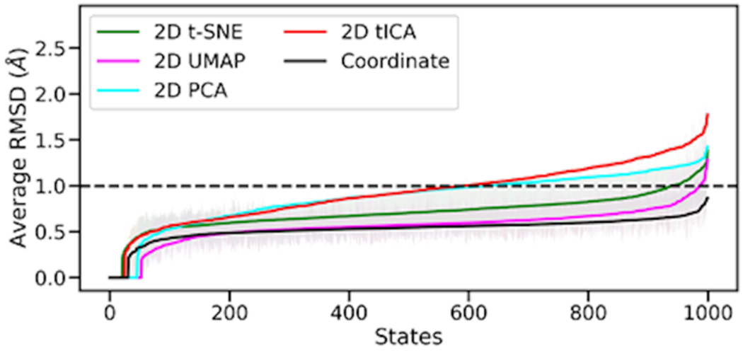
Averaged RMSD of 1000 microstates for various 2D representations and Cartesian coordinates. Microstates were sorted based on the average RMSD values.

3.1.3. Division of the Conformational Space into Macrostates

Protein conformational landscape is characterized by a series of low free energy basins comprising low-energy conformations. To correctly cluster different structures into metastable states, k-means clustering method was used to build clusters with the mean RMSD within cluster smaller than 1 Å. As mentioned above, structures with their RMSD smaller than 1 Å are expected to belong to the same free energy basin and therefore the same metastable state. This procedure ensures that no artificial free energy barriers are hidden within each cluster. In this study, a total of 16 clusters were found to be the lowest number of clusters that have mean intra-cluster RMSD within 1 Å and maximal inter-clusters difference (Figure 3). These 16 clusters are hereby referred to as macrostates.

Figure 3.

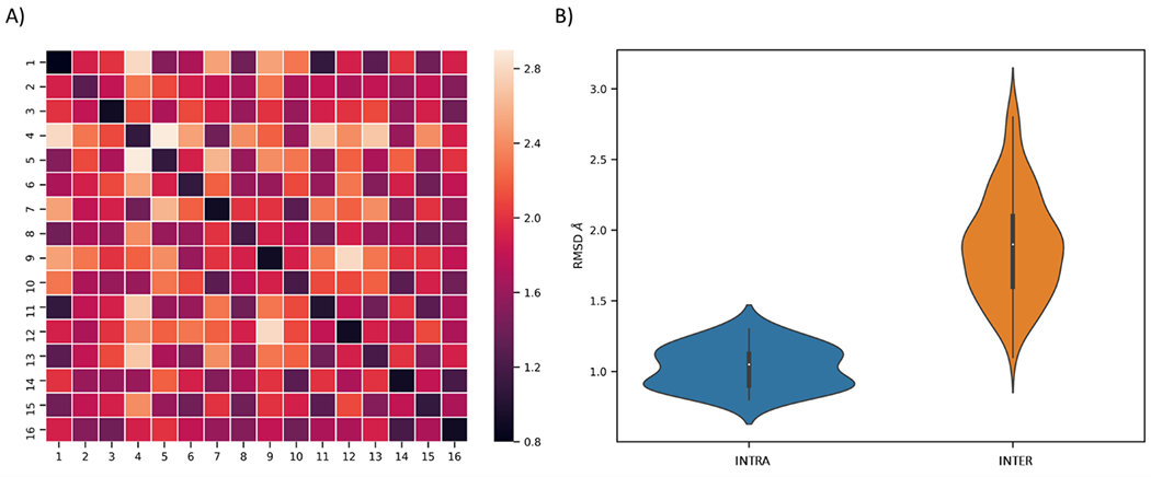
Selection of number of macrostate based on cluster RMSD. A) Heatmap of RMSD within each state. B) Violin plot of RMSD values within states (blue) and inter states (orange).

To evaluate how well the clustering in the low dimensional space represents the original data in the high-dimensional space, we calculated a similarity score by comparing the population of each cluster in the reduced embedding with the corresponding cluster in the high-dimensional manifold. The first step was the assignment of the clusters in the low dimensional embedding to the corresponding high-dimensional clusters. After the assignment being made, for each pair of clusters, one in the high-dimensional space and one in the low-dimensional space, the number of points shared by both clusters was counted. The total number of these shared points was summed and converted to the percentage to the total number of data points. Figure 4 shows that UMAP improves t-SNE performances and outperforms PCA and tICA in similarity score. This demonstrates that UMAP could appropriately assign protein structures into their corresponding functional metastable states (macrostates) for further analyses.

Figure 4.

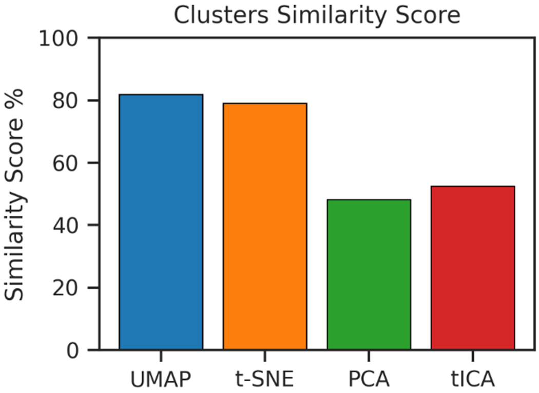
Similarity, expressed in percentage, between cluster populations in low-dimensional representations and high-dimensional Cartesian space.

Another important criterion for dimensionality reduction method is clusters separation. Specifically, an adequate low-dimensional projection should retain the separation that these macrostates have in the high-dimensional space. The projection of the macro-cluster is plotted in Figure S2.

To quantitatively assess the quality of clustering projections, we employed the silhouette coefficient (SC). As described in the method section, the SC is a clustering quality assessment criterion which evaluates the separation distances between clusters. SCs ranges from −1 to +1, where positive values indicate better separation between clusters and negative values indicating their overlap. The SC for each method as well as in the Cartesian space are listed in Table S1. In Figure 5, we plot the difference between the SC of each dimensionality reduction method and the SC of the original Cartesian space. In this comparison, a negative value indicates that a projection using certain dimensionality reduction method increases the overlap among the macrostates compared to the results in Cartesian space. A positive value indicates a higher separation, possibly an over-separation, among macrostates in the projection compared to the results in Cartesian space. When only one dimension is used to project the conformational space, UMAP and t-SNE offer a more faithful projection of the macro-clusters, demonstrated by the small values of the SC difference. When two dimensions are considered, a similar amount of divergence in different directions is observed for the projection for all methods. Interestingly, the non-linear methods UMAP and t-SNE tend to over-separate the clusters, while the linear PCA and tICA tend to increase their overlap. When three dimensions are used, both UMAP and t-SNE still lead to higher separation than the Cartesian results. PCA method results in a slightly higher separation. tICA still results in a higher overlapping than the Cartesian results.

Figure 5.

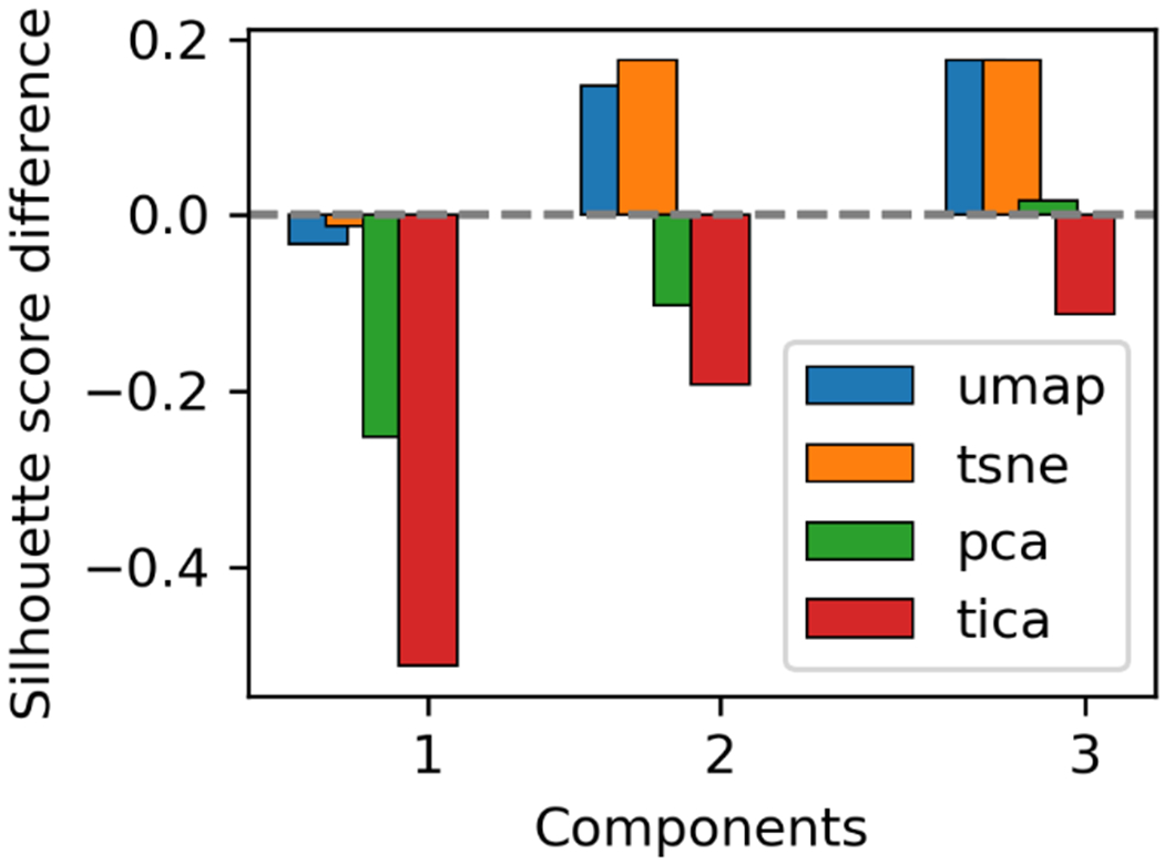
Comparison of silhouette coefficient for UMAP, t-SNE, PCA, and tICA projections vs Cartesian space results. Bar heights represent the deviation in coefficient from the Cartesian case. Positive values represent higher separation of the clusters in the projected space. Negative values represent overcrowding of the clusters in projected spaces.

3.1.4. Machine learning classification

In our previous studies, it was demonstrated that machine learning based classification for the macrostates is an effective approach to delineate protein allosteric mechanism related to individual residues. ^27,66–68 To build effective machine learning classification models, it is desired to have dimensionality reduction methods which could enhance the quality of classification models. We used Random Forest as machine learning classification model. The best combination of hyper-parameters for the input data from each dimensionality reduction method was identified using grid searches (Table S2). Using UMAP and t-SNE, the machine learning classification models for the macrostates generated using the two most dominant dimensions reach 95% accuracy (Figure 6). As a comparison, the similar prediction accuracy is much smaller for PCA and tICA, as 66% and 70%, respectively. This is in the agreement with their performance of the 1D projection of the 16 macrostates (Figure 5), in which macrostates generated using PCA and tICA methods have more overlaps than those from UMAP and t-SNE methods.

Figure 6.

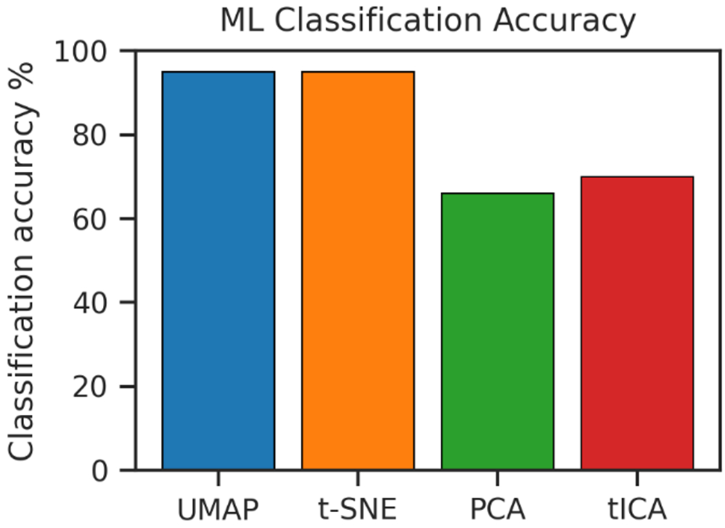
Machine learning prediction accuracy of the different macrostates based on the 2D input of the low-dimensional representation using Random Forest.

3.1.5. Kinetics

Proteins are in constant motions, whether when carrying out their biochemical functions or not. One common approach to probe protein dynamics is building Markov State Models (MSM) to estimate probabilities for protein transition among different macrostates. To build effective MSM, it is important for a dimensionality reduction method to retain information about how proteins transition among these macrostates. To evaluate the retaining of such information, we analyzed the relaxation timescales in MSM, also referred to as implied timescales, using different dimensionality reduction methods with comparison to the results using Cartesian coordinates. ¹⁹ The relaxation timescale can be interpreted as the time needed for a system to change its state. ⁶⁹ As protein functions are presumed to be strongly correlated with protein slow motions, a well-behaving dimensionality reduction method is expected to preserve slow degrees of freedom of protein simulations for accurate description of protein kinetics related to their functions.

Overall, all methods behave well to produce the implied timescales range close to the Cartesian coordinates results except for PCA (Figure 7). UMAP produces implied timescales that is the closest to the Cartesian coordinates results, especially with the lag time longer than 60ns. The t-SNE method is the second best, and its implied timescales also converge to the Cartesian coordinates results with the lag time longer than 70ns. Although tICA also produces result close to the one of Cartesian coordinates, it overestimates the implied timescales of the system, and its results do not converge to the Cartesian coordinates results. This comparison demonstrates that UMAP could retain protein dynamics information to describe the kinetics of the target system.

Figure 7.

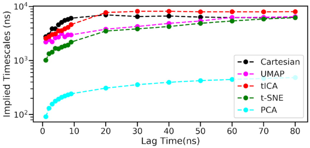
Comparison of implied timescales of different methods.

The transition matrix produced in each MSM provides transition probability between each pair of macrostates as detailed kinetics information of the system. To further evaluate the performance of each dimensionality reduction method to retain kinetics information of the system, we implemented a transition matrix error analysis by comparing the transition matrices from different dimensionality reduction methods with the Cartesian coordinates results as the reference. For this comparison, we used a total of 16 macrostates identified in section 3.1.3. The absolute value for the difference of each transition matrix element is listed and illustrated as heatmaps (Figure 8). To quantify the deviation from the high dimensional transition matrix, the deviation sum was calculated for each method, as 8.26, 9.33, 14.06, 9.39 for UMAP, t-SNE, PCA, and tICA, respectively. UMAP outperforms the other dimensionality reduction methods. This result indicates that UMAP well captures the system kinetics, related to the free energy surface. Moreover, tICA performs similarly to t-SNE and UMAP.

Figure 8.

Heatmap representation of divergence of the different transition matrices obtained using different dimensionality reduction methods from the high dimensional transition matrix.

3.2. How many dimensions are needed?

Ideally, a good dimensionality reduction method should retain both structural and kinetic information of a trajectory using a minimal number of dimensions possible. Therefore, it was evaluated that how much information could be retained by the most dominant components generated in each method. One of the goals of this analysis is determining how many dimensions are optimal for retaining structural and kinetic properties of the model system using each method. Both the Pearson correlation and transition matrix error for each method were used to evaluate the structural and kinetic information retention. The Pearson correlation is used to identify the structural similarities between the original data in the high dimensional space and low dimensional embedding using various numbers of dimensions.

Using the Pearson correlation analysis, the correlation between the original data and the new data projected onto different numbers of components starting with one was calculated and plotted for the selected methods (Figure 9A). For UMAP, t-SNE, and PCA, the Pearson correlation is above 0.80 when the original data are projected onto the most dominant dimension and above 0.90 with the top two dominant dimensions being used. Both PCA and t-SNE display the best Pearson correlation when using one or two components. For tICA, the Pearson correlation is much lower comparing to the other three methods, making it less ideal for the analysis of the protein conformational space.

Figure 9.

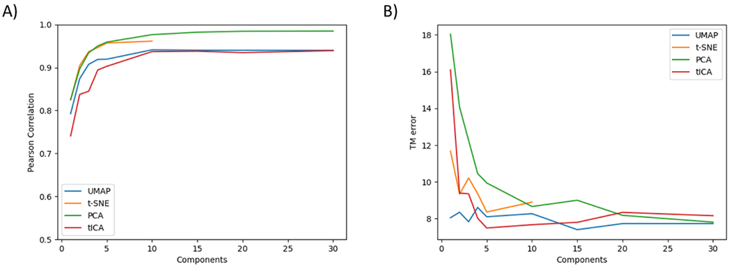
Performance of different methods regarding the number of components used in projection. A) Pearson correlation between high dimensional representation and reduced representation of the data at varying number of projected dimensions. B) Transition matrices error between high dimensional representation and reduced representation of the data at varying number of projected dimensions.

To evaluate the kinetic information retention using various numbers of dimensions, the transition matrix error analysis was carried out for each method when using different numbers of components for data projection. The total of absolute transition matrix error for each case is plotted for comparison (Figure 9B). When using only one or two components for data projection, PCA displays the highest errors, probably due to its linearity nature. tICA also displays significant errors when using only one or two components for data projection. Surprisingly, t-SNE also displays significant errors when using only one or two components for data projection. UMAP consistently displays the lowest transition matrix error when using one, two or three components for data projection. Overall, the above analyses ensure the applicability of UMAP with a minimal loss of structural and kinetic information, two critical aspects in the study of protein biology.

3.3. Benchmark

From a practical point of view, another crucial factor in choosing a dimensionality reduction method is its computational cost. We carried out some benchmark calculations to compare the computational cost of UMAP, t-SNE, PCA, and tICA for various numbers of components for projection (Figure 10A). For PCA, tICA, and UMAP, the computational cost remains close to constant regardless the number of components used for projection. However, the computational cost increases exponentially with the number of components used for projecting when using t-SNE. In our benchmark calculation, we could only perform the calculation up to 5 dimensions with t-SNE method. The computational cost with only one or two components for data projection is also significantly higher than all other methods by factors of 5 to 8. This greatly limits the applicability of t-SNE for protein dynamics analyses. Although the computational cost for PCA and tICA is close to negligible as linear methods, the computational cost for UMAP as nonlinear dimensionality reduction method is not much higher, making UMAP as a very feasible option for dimensionality reduction analysis. All the benchmark calculations were performed with NVIDIA GPUs which are configured with dual Intel Xeon E5-2695v4 2.1 GHz 18-core “Broadwell” processors, 256 GB of DDR4-2400 memory.

Figure 10.

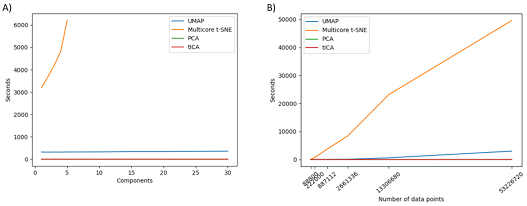
Benchmark using different dimensionality reduction methods. A) Time in seconds required for dimensionality reduction at various numbers of projected dimensions. B) Time in seconds required for 2D projections using different number of frames as data points.

The benchmark calculations were also carried for two components projection with different numbers of data points used, as 2D is the most widely used for protein dynamics analyses. Regarding the speed for varying number of points, the number of data-points was varied by progressively increasing the stride between consecutive frames in the trajectories. Figure 10B shows that UMAP achieves similar speed performance of PCA and tICA. While its computational time increases with the increase the sample number, its speed remains close to the linear methods. The time required by t-SNE significantly exceeds the time required by tICA, PCA, and UMAP.

3.4. Leading to Insight into Protein Function Mechanism

The purpose of using dimensionality reduction methods for protein dynamics analyses is providing mechanistic insights into protein structures and functions. As there is no universal standard to evaluate such performance, some demonstrative analyses were carried out for the model system used in this study. VVD is a well characterized circadian clock protein that has been shown to undergo conformational changes depending on the light condition. Following the rational of the sections discussed above, the conformational space of this protein sampled in the MD simulations has been clustered in 16 macrostates projected onto the 2D surface using the top two components from UMAP analysis (Figure 11A). In this plot, blue is used to indicate the dark state, lighter blue is used to indicate the transition dark state, red is used to indicate the light state, and lighter red for the transition light state. The light (red) and dark (blue) states in the UMAP projections are well separated (Figure 11A), which is ideal to study proteins with distinct functional states.

Figure 11.

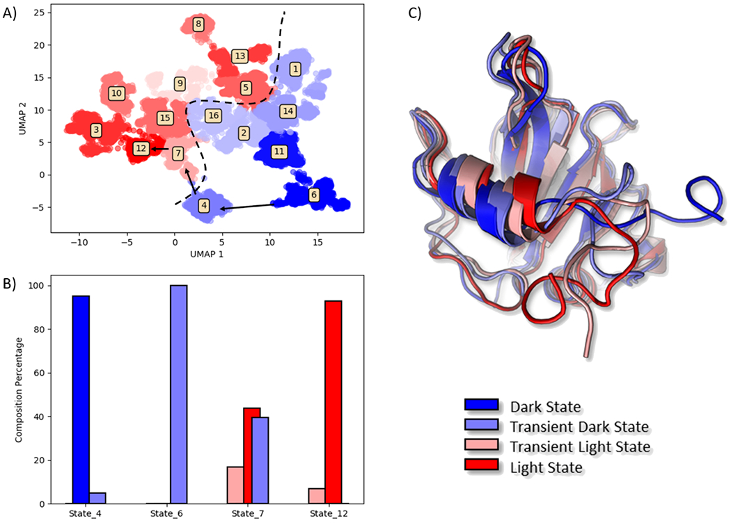
Demonstration of protein function analysis using UMAP method. A) UMAP 2D projection. Reduced space was clustered in 16 macrostates according to the criteria presented above. The clusters were color coded based on their population. Dark states are blue, and light states are red. Dashed line represents division between dark and light areas. Arrows represent pathway for allosteric conversion from fully dark to fully light states. B) Population states analysis of the macrostates involved in VVD allosteric process. C) Visualization of the four representative states involved in the allosteric process.

With well-separated representation of functional states in the reduced dimensions, the Transition Path Theory (TPT) could be used to provide detailed kinetics of transitions among different macrostates. Using TPT, it is identified that the major transition pathway from the dark state (State 6) to the light state (State 12) gradually transition via transition pathway through State 4 belonging to the transient dark state and State 7 belonging to the transient light state (Figure 11B).

The α helix movement and undocking of the N-terminus as key changes are illustrated in the representative structures (Figure 11C). These movements have been recognized to be crucial steps in VVD allostery in the comprehensive mechanistic study done on this system by Zhou et al. ²⁷ This analysis not only demonstrates the ability of UMAP of capturing fundamental biological properties of the system, but showcases that UMAP can be used as visualization tool for protein conformational space.

4. Discussion

Molecular dynamics simulations have been used as indispensable approaches for the studies of protein functions within the dynamics framework. Although the time scales affordable for the MD simulations have been increasing significantly in recent years, it is still far from being comparable with the actual time scales for the protein biological functions. Even with this limitation, the curse of the dimensionality still prevents direct analyses of many properties of protein dynamics. Therefore, dimensionality reduction methods have been serving as essential tools to process protein MD simulations to gain insight into protein dynamical properties including both conformational space and kinetics information.

RMSD is a simple and effective measurement of conformational deviation between two structures. Using this quantity, the ability of each dimensionality reduction method to represent the conformational space sampled from the simulation could be evaluate accurately. The reason that the nonlinear dimensionality reduction methods, including UMAP and t-SNE, could produce much better clustering results than the linear methods, including PCA and tICA, is probably because the most protein conformational changes have intrinsic nonlinearity, such as bond bending, dihedral angle rotations, and global motion of protein structures. UMAP produces better results than t-SNE when comparing with the Cartesian coordinates results as the benchmark (Figure 2), suggesting that this method is approaching methodological limit of dimensionality reduction methods in general. This is also supported by the highest similarity score of UMAP among all four methods (Figure 4). It should be noted that the comparison presented here is by no means complete or exhaust. Therefore, it should not be concluded that UMAP is the best option to represent the conformational space sampling in all cases.

In addition to representing conformational changes well, it is more important and challenging to retain the kinetics information of protein dynamics when projecting the simulation trajectories onto reduced dimensional space. As this is an active research area, a universal standard to evaluate kinetics information is yet to be determined. Therefore, the convergence test of implied timescales in MSM is used as the benchmark for kinetics information retention. Although it is not surprising that tICA demonstrates closer trend to the results of Cartesian coordinates as tICA was developed to capture the slow and global motion of proteins, it is somewhat suspicious that the tICA results do not converge to the Cartesian coordinates results with longer lag times. Overall, UMAP is demonstrated as a more balanced option than both tICA and t-SNE methods. With smaller lag times, UMAP results are also close to the Cartesian coordinates results, similar to tICA (Figure 7). With longer lag times, UMAP results display better convergence to the Cartesian coordinates results than t-SNE (Figure 7). The superiority of UMAP for kinetics information retention is also supported by the high accuracy of machine learning based prediction model based on MSM using UMAP projection (Figure 6). The fact that UMAP results are better than other methods in both conformation and kinetics representations is promising. Although there is no direct evidence, the satisfactory performance of UMAP to preserve protein kinetics information could be partially due to the good representation of protein conformational space.

Because of the limitation of human perception of dimensionality, the dimensions of graphical representation of protein dynamics analysis have been limited to two. This is validated by the evaluation of Pearson correlation between the projected data in low dimensional spaces and the original data and transition matrix error analyses (Figure 9). Both t-SNE and PCA methods display high Pearson correlation with one or two dimensions for data projection. As a linear method, PCA is not always suitable for protein dynamics simulations, leaving t-SNE as a better choice in this regard. UMAP produces comparable Pearson correlations with one or two dimensions for data projection. Interestingly, the UMAP method produces much lower transition matrix error than all other three methods, making it a well-balanced method for low dimensional spaces projection. Considering almost constant computational cost of UMAP method, which is similar to PCA and tICA and much lower than the exponentially increasing computational cost of t-SNE (Figure 10), UMAP clearly serves as a viable option for dimensionality reduction analyses of complexed biomolecular systems, including proteins.

5. Conclusions

In this study, the suitability and performance of the Uniform Manifold Approximation and Projection (UMAP) as a new fuzzy topology-based dimensionality reduction method for the simulation of macromolecules was systematically evaluated and compared with other widely used dimensionality reduction methods, including Principal Component Analysis (PCA), time-structure Independent Components Analysis (tICA), and t-Distributed Stochastic Neighbor Embedding (t-SNE). Using the Cartesian coordinates representation as the benchmark, it was demonstrated that UMAP could well retain the protein conformational information after the projection of original data. More importantly, the UMAP could also retain the protein kinetics information, which is critical to gain insight into protein functions within dynamics framework. The balanced performance of UMAP to preserve protein kinetics is achieved through building Markov state model (MSM) based on UMAP projection with well-preserved conformational space information. As a non-linear dimensionality reduction method, UMAP displays similar overall performance and is more-balanced between conformational and kinetics information retention than t-SNE. In addition, the computational cost of UMAP remains close to constant regardless the number of dimensions being used for data projection. As comparison t-SNE requires exponentially increasing computational cost regarding the number of dimensions for the target data projection. Overall, the UMAP method is a well behaving and balanced dimensionality reduction method for in-depth biomacromolecule simulation analyses to gain insight into both structure-function and dynamics-function relations.

Supplementary Material

UMAP Supporting Information

Figure S1. Hyperparameters evaluation for UMAP performance. For each combination of hyperparameters, the circle size represents the normalized Pearson correlation coefficient. The circle color, in the scale from blue to red, represents the cluster similarity score.

Figure S2. Projections of the macro-clusters found in the Cartesian space into low dimensional space obtained using UMAP, t-SNE, PCA, tICA. A) Projections on 1D spaces; B) Projections on 2D spaces; C) Projections on 3D spaces.

Table S1. Best hyperparameters for ML classification model with different dimensionality reduction projections as input data.

Table S2. Silhouette Coefficients calculated on the projections performed using UMAP, t-SNE, PCA, and tICA.

Abbreviations

UMAP

Uniform Manifold Approximation and Projection

t-SNE

t-Distributed Stochastic Neighbor Embedding

PCA

Principal Component Analysis

t-ICA

time-structure Independent Component Analysis

MD

molecular dynamics

CV

collective variable

MSM

Markov state model

KL

Kullback–Leibler

VVD

vivid

CE

cross entropy

RMSD

root mean squared deviation

PC

Pearson correlation

SC

silhouette coefficient

ML

machine learning

TPT

transition path theory

References

- (1).Joshi T; Xu D Quantitative Assessment of Relationship between Sequence Similarity and Function Similarity. BMC Genomics 2007, 8 (1), 1–10. 10.1186/1471-2164-8-222. [DOI] [PMC free article] [PubMed] [Google Scholar]
- (2).Fowler DM; Araya CL; Fleishman SJ; Kellogg EH; Stephany JJ; Baker D; Fields S High-Resolution Mapping of Protein Sequence-Function Relationships. Nat. Methods 2010, 7 (9), 741–746. 10.1038/nmeth.1492. [DOI] [PMC free article] [PubMed] [Google Scholar]
- (3).Hegyi H; Gerstein M The Relationship between Protein Structure and Function: A Comprehensive Survey with Application to the Yeast Genome. J. Mol. Biol 1999, 288 (1), 147–164. 10.1006/jmbi.1999.2661. [DOI] [PubMed] [Google Scholar]
- (4).Orengo CA; Todd AE; Thornton JM From Protein Structure to Function. Curr. Opin. Struct. Biol 1999, 9 (3), 374–382. 10.1016/S0959-440X(99)80051-7. [DOI] [PubMed] [Google Scholar]
- (5).Hensen U; Meyer T; Haas J; Rex R; Vriend G; Grubmüller H Exploring Protein Dynamics Space: The Dynasome as the Missing Link between Protein Structure and Function. PLoS One 2012, 7 (5), e33931. 10.1371/journal.pone.0033931. [DOI] [PMC free article] [PubMed] [Google Scholar]
- (6).Karplus M; Kuriyan J Molecular Dynamics and Protein Function. Proc. Natl. Acad. Sci. U.S.A 2005, 102 (19), 6679–6685. 10.1073/pnas.0408930102. [DOI] [PMC free article] [PubMed] [Google Scholar]
- (7).Klepeis JL; Lindorff-Larsen K; Dror RO; Shaw DE Long-Timescale Molecular Dynamics Simulations of Protein Structure and Function. Curr. Opin. Struct. Biol 2009, 19 (2), 120–127. 10.1016/j.sbi.2009.03.004. [DOI] [PubMed] [Google Scholar]
- (8).Hansson T; Oostenbrink C; Van Gunsteren WF Molecular Dynamics Simulations. Curr. Opin. Struct. Biol 2002, 12 (2), 190–196. 10.1016/S0959-440X(02)00308-1. [DOI] [PubMed] [Google Scholar]
- (9).García AE Large-Amplitude Nonlinear Motions in Proteins. Phys. Rev. Lett 1992, 68 (17), 2696–2699. 10.1103/PhysRevLett.68.2696. [DOI] [PubMed] [Google Scholar]
- (10).Stein SAM; Loccisano AE; Firestine SM; Evanseck JD Chapter 13 Principal Components Analysis: A Review of Its Application on Molecular Dynamics Data. Annual Reports in Computational Chemistry. 2006, pp 233–261. 10.1016/S1574-1400(06)02013-5. [DOI] [Google Scholar]
- (11).Tian H; Tao P Ivis Dimensionality Reduction Framework for Biomacromolecular Simulations. J. Chem. Inf. Model 2020, 60 (10), 4569–4581. 10.1021/acs.jcim.0c00485. [DOI] [PMC free article] [PubMed] [Google Scholar]
- (12).Song Z; Zhou H; Tian H; Wang X; Tao P Unraveling the Energetic Significance of Chemical Events in Enzyme Catalysis via Machine-Learning Based Regression Approach. Commun. Chem 2020, 3 (1), 1–10. 10.1038/s42004-020-00379-w. [DOI] [PMC free article] [PubMed] [Google Scholar]
- (13).Das P; Moll M; Stamati H; Kavraki LE; Clementi C Low-Dimensional, Free-Energy Landscapes of Protein-Folding Reactions by Nonlinear Dimensionality Reduction. Proc. Natl. Acad. Sci. U. S. A 2006, 103 (26), 9885–9890. 10.1073/pnas.0603553103. [DOI] [PMC free article] [PubMed] [Google Scholar]
- (14).Brown WM; Martin S; Pollock SN; Coutsias EA; Watson J-P Algorithmic Dimensionality Reduction for Molecular Structure Analysis. J. Chem. Phys 2008, 129 (6), 064118. 10.1063/1.2968610. [DOI] [PMC free article] [PubMed] [Google Scholar]
- (15).Stamati H; Clementi C; Kavraki LE Application of Nonlinear Dimensionality Reduction to Characterize the Conformational Landscape of Small Peptides. Proteins Struct. Funct. Bioinforma 2010, 78 (2), 223–235. 10.1002/prot.22526. [DOI] [PMC free article] [PubMed] [Google Scholar]
- (16).Ferguson AL; Panagiotopoulos AZ; Kevrekidis IG; Debenedetti PG Nonlinear Dimensionality Reduction in Molecular Simulation: The Diffusion Map Approach. Chem. Phys. Lett 2011, 509 (1–3), 1–11. 10.1016/j.cplett.2011.04.066. [DOI] [Google Scholar]
- (17).Duan M; Fan J; Li M; Han L; Huo S Evaluation of Dimensionality-Reduction Methods from Peptide Folding-Unfolding Simulations. J. Chem. Theory Comput 2013, 9 (5), 2490–2497. 10.1021/ct400052y. [DOI] [PMC free article] [PubMed] [Google Scholar]
- (18).Doerr S; Ariz-Extreme I; Harvey MJ; De Fabritiis G Dimensionality Reduction Methods for Molecular Simulations. arXiv. 2017. [Google Scholar]
- (19).Zhou H; Wang F; Tao P T-Distributed Stochastic Neighbor Embedding Method with the Least Information Loss for Macromolecular Simulations. J. Chem. Theory Comput 2018, 14 (11), 5499–5510. 10.1021/acs.jctc.8b00652. [DOI] [PMC free article] [PubMed] [Google Scholar]
- (20).Tribello GA; Gasparotto P Using Dimensionality Reduction to Analyze Protein Trajectories. Front. Mol. Biosci 2019, 6 (JUN), 46. 10.3389/fmolb.2019.00046. [DOI] [PMC free article] [PubMed] [Google Scholar]
- (21).Prinz JH; Wu H; Sarich M; Keller B; Senne M; Held M; Chodera JD; Schtte C; Noé F Markov Models of Molecular Kinetics: Generation and Validation. J. Chem. Phys 2011, 134 (17), 174105. 10.1063/1.3565032. [DOI] [PubMed] [Google Scholar]
- (22).Bowman GR; Pande VS; Noé F An Introduction to Markov State Models and Their Application to Long Timescale Molecular Simulation. Springer; 2014, 797, 148. 10.1007/978-94-007-7606-7. [DOI] [Google Scholar]
- (23).Shukla D; Hernández CX; Weber JK; Pande VS Markov State Models Provide Insights into Dynamic Modulation of Protein Function. Acc. Chem. Res 2015, 48 (2), 414–422. 10.1021/ar5002999. [DOI] [PMC free article] [PubMed] [Google Scholar]
- (24).Shukla S; Shamsi Z; Moffett AS; Selvam B; Shukla D Application of Hidden Markov Models in Biomolecular Simulations. In Hidden Markov Models; Springer, 2017; pp 29–41. [DOI] [PubMed] [Google Scholar]
- (25).Shamsi Z; Moffett AS; Shukla D Enhanced Unbiased Sampling of Protein Dynamics Using Evolutionary Coupling Information. Sci. Rep 2017, 7 (1), 1–13. [DOI] [PMC free article] [PubMed] [Google Scholar]
- (26).Zhou S; Wang Q; Wang Y; Yao X; Han W; Liu H The Folding Mechanism and Key Metastable State Identification of the PrP127–147 Monomer Studied by Molecular Dynamics Simulations and Markov State Model Analysis. Phys. Chem. Chem. Phys 2017, 19 (18), 11249–11259. 10.1039/c7cp01521f. [DOI] [PubMed] [Google Scholar]
- (27).Zhou H; Dong Z; Verkhivker G; Zoltowski BD; Tao P Allosteric Mechanism of the Circadian Protein Vivid Resolved through Markov State Model and Machine Learning Analysis. PLoS Comput. Biol 2019, 15 (2), e1006801. 10.1371/journal.pcbi.1006801. [DOI] [PMC free article] [PubMed] [Google Scholar]
- (28).Roweis ST; Saul LK Nonlinear Dimensionality Reduction by Locally Linear Embedding. Science. 2000. 290 (5500), 2323–2326 10.1126/science.290.5500.2323. [DOI] [PubMed] [Google Scholar]
- (29).Cunningham JP; Ghahramani Z Linear Dimensionality Reduction: Survey, Insights, and Generalizations. J. Mach. Learn. Res 2015, 16 (89), 2859–2900. [Google Scholar]
- (30).Sugiyama M Nonlinear Dimensionality Reduction. In Introduction to Statistical Machine Learning; Elsevier, 2016; pp 429–446. 10.1016/b978-0-12-802121-7.00047-9. [DOI] [Google Scholar]
- (31).McInnes L; Healy J; Saul N; Großberger L UMAP: Uniform Manifold Approximation and Projection. J. Open Source Softw 2018, 3 (29), 861. 10.21105/joss.00861. [DOI] [Google Scholar]
- (32).Becht E; McInnes L; Healy J; Dutertre CA; Kwok IWH; Ng LG; Ginhoux F; Newell EW Dimensionality Reduction for Visualizing Single-Cell Data Using UMAP. Nat. Biotechnol 2019, 37 (1), 38–47. 10.1038/nbt.4314. [DOI] [PubMed] [Google Scholar]
- (33).Cao J; Spielmann M; Qiu X; Huang X; Ibrahim DM; Hill AJ; Zhang F; Mundlos S; Christiansen L; Steemers FJ; Trapnell C; Shendure J The Single-Cell Transcriptional Landscape of Mammalian Organogenesis. Nature 2019, 566 (7745), 496–502. 10.1038/s41586-019-0969-x. [DOI] [PMC free article] [PubMed] [Google Scholar]
- (34).Packer JS; Zhu Q; Huynh C; Sivaramakrishnan P; Preston E; Dueck H; Stefanik D; Tan K; Trapnell C; Kim J; Waterston RH; Murray JI A Lineage-Resolved Molecular Atlas of C. Elegans Embryogenesis at Single-Cell Resolution. Science. 2019, 365 (6459). 10.1126/science.aax1971. [DOI] [PMC free article] [PubMed] [Google Scholar]
- (35).Diaz-Papkovich A; Anderson-Trocmé L; Ben-Eghan C; Gravel S UMAP Reveals Cryptic Population Structure and Phenotype Heterogeneity in Large Genomic Cohorts. PLoS Genet. 2019, 15 (11), e1008432. 10.1371/journal.pgen.1008432. [DOI] [PMC free article] [PubMed] [Google Scholar]
- (36).Zoltowski BD; Schwerdtfeger C; Widom J; Loros JJ; Bilwes AM; Dunlap JC; Crane BR Conformational Switching in the Fungal Light Sensor Vivid. Science. 2007, 316 (5827), 1054–1057. 10.1126/science.1137128. [DOI] [PMC free article] [PubMed] [Google Scholar]
- (37).Zoltowski BD; Crane BR Light Activation of the LOV Protein Vivid Generates a Rapidly Exchanging Dimer. Biochemistry 2008, 47 (27), 7012–7019. 10.1021/bi8007017. [DOI] [PMC free article] [PubMed] [Google Scholar]
- (38).Zoltowski BD; Vaccaro B; Crane BR Mechanism-Based Tuning of a LOV Domain Photoreceptor. Nat. Chem. Biol 2009, 5 (11), 827–834. 10.1038/nchembio.210. [DOI] [PMC free article] [PubMed] [Google Scholar]
- (39).Wold S; Esbensen K; Geladi P Principal Component Analysis. Chemom. Intell. Lab. Syst 1987, 2 (1–3), 37–52. 10.1016/0169-7439(87)80084-9. [DOI] [Google Scholar]
- (40).Pedregosa F; Michel V; Varoquaux G; Thirion B; Dubourg V; Passos A; Perrot M; Grisel O; Blondel M; Prettenhofer P; Weiss R; Vanderplas J; Cournapeau D; Pedregosa F; Varoquaux G; Gramfort A; Thirion B; Grisel O; Dubourg V; Passos A; Brucher M; Perrot M; Duchesnay É Scikit-Learn: Machine Learning in Python. J Mach Learn Res. 2011, 12, 2825–2830. [Google Scholar]
- (41).Naritomi Y; Fuchigami S Slow Dynamics in Protein Fluctuations Revealed by Time-Structure Based Independent Component Analysis: The Case of Domain Motions. J. Chem. Phys 2011, 134 (6), 02B617. 10.1063/1.3554380. [DOI] [PubMed] [Google Scholar]
- (42).Schwantes CR; Pande VS Improvements in Markov State Model Construction Reveal Many Non-Native Interactions in the Folding of NTL9. J. Chem. Theory Comput 2013, 9 (4), 2000–2009. 10.1021/ct300878a. [DOI] [PMC free article] [PubMed] [Google Scholar]
- (43).Sultan MM; Pande VS TICA-Metadynamics: Accelerating Metadynamics by Using Kinetically Selected Collective Variables. J. Chem. Theory Comput 2017, 13 (6), 2440–2447. 10.1021/acs.jctc.7b00182. [DOI] [PubMed] [Google Scholar]
- (44).Harrigan MP; Sultan MM; Hernández CX; Husic BE; Eastman P; Schwantes CR; Beauchamp KA; McGibbon RT; Pande VS MSMBuilder: Statistical Models for Biomolecular Dynamics. Biophys. J 2017, 112 (1), 10–15. 10.1016/j.bpj.2016.10.042. [DOI] [PMC free article] [PubMed] [Google Scholar]
- (45).Van der Maaten Laurens and Hinton G. Visualizing Data Using T-SNE. J. Mach. Learn. Res 2008, 9 (11), 2579–2605. [Google Scholar]
- (46).Berman HM; Battistuz T; Bhat TN; Bluhm WF; Bourne PE; Burkhardt K; Feng Z; Gilliland GL; Iype L; Jain S; Fagan P; Marvin J; Padilla D; Ravichandran V; Schneider B; Thanki N; Weissig H; Westbrook JD; Zardecki C The Protein Data Bank. Acta Crystallogr. Sect. D Biol. Crystallogr 2002, 58 (6), 899–907. 10.1107/S0907444902003451. [DOI] [PubMed] [Google Scholar]
- (47).Freddolino PL; Gardner KH; Schulten K Signaling Mechanisms of LOV Domains: New Insights from Molecular Dynamics Studies. Photochem. Photobiol. Sci 2013, 12 (7), 1158–1170. 10.1039/c3pp25400c. [DOI] [PMC free article] [PubMed] [Google Scholar]
- (48).Martínez-Rosell G; Giorgino T; De Fabritiis G PlayMolecule ProteinPrepare: A Web Application for Protein Preparation for Molecular Dynamics Simulations. J. Chem. Inf. Model 2017, 57 (7), 1511–1516. 10.1021/acs.jcim.7b00190. [DOI] [PubMed] [Google Scholar]
- (49).Brooks BR; Brooks CL; Mackerell AD; Nilsson L; Petrella RJ; Roux B; Won Y; Archontis G; Bartels C; Boresch S; Caflisch A; Caves L; Cui Q; Dinner AR; Feig M; Fischer S; Gao J; Hodoscek M; Im W; Kuczera K; Lazaridis T; Ma J; Ovchinnikov V; Paci E; Pastor RW; Post CB; Pu JZ; Schaefer M; Tidor B; Venable RM; Woodcock HL; Wu X; Yang W; York DM; Karplus M CHARMM: The Biomolecular Simulation Program. J. Comput. Chem 2009, 30 (10), 1545–1614. 10.1002/jcc.21287. [DOI] [PMC free article] [PubMed] [Google Scholar]
- (50).Eastman P; Swails J; Chodera JD; McGibbon RT; Zhao Y; Beauchamp KA; Wang LP; Simmonett AC; Harrigan MP; Stern CD; Wiewiora RP; Brooks BR; Pande VS OpenMM 7: Rapid Development of High Performance Algorithms for Molecular Dynamics. PLoS Comput. Biol 2017, 13 (7), e1005659. 10.1371/journal.pcbi.1005659. [DOI] [PMC free article] [PubMed] [Google Scholar]
- (51).Eastman P; Friedrichs MS; Chodera JD; Radmer RJ; Bruns CM; Ku JP; Beauchamp KA; Lane TJ; Wang LP; Shukla D; Tye T; Houston M; Stich T; Klein C; Shirts MR; Pande VS OpenMM 4: A Reusable, Extensible, Hardware Independent Library for High Performance Molecular Simulation. J. Chem. Theory Comput 2013, 9 (1), 461–469. 10.1021/ct300857j. [DOI] [PMC free article] [PubMed] [Google Scholar]
- (52).Ryckaert JP; Ciccotti G; Berendsen HJ . Numerical Integration of the Cartesian Equations of Motion of a System with Constraints: Molecular Dynamics of n-Alkanes. J. Comput. Phys 1977, 23 (3), 327–341. 10.1016/0021-9991(77)90098-5. [DOI] [Google Scholar]
- (53).Essmann U; Perera L; Berkowitz ML; Darden T; Lee H; Pedersen LG A Smooth Particle Mesh Ewald Method. J. Chem. Phys 1995, 103 (19), 8577–8593. 10.1063/1.470117. [DOI] [Google Scholar]
- (54).Benesty J; Chen J; Huang Y; Cohen I Pearson Correlation Coefficient. In Noise reduction in speech processing; Springer, 2009; pp 1–4. [Google Scholar]
- (55).Aggarwal CC; Hinneburg A; Keim DA On the Surprising Behavior of Distance Metrics in High Dimensional Space. In Lecture Notes in Computer Science (including subseries Lecture Notes in Artificial Intelligence and Lecture Notes in Bioinformatics); 2001; Vol. 1973, pp 420–434. 10.1007/3-540-44503-x_27. [DOI] [Google Scholar]
- (56).Rousseeuw PJ Silhouettes: A Graphical Aid to the Interpretation and Validation of Cluster Analysis. J. Comput. Appl. Math 1987, 20 (C), 53–65. 10.1016/0377-0427(87)90125-7. [DOI] [Google Scholar]
- (57).Liaw A; Wiener M Classification and Regression by RandomForest. R news 2002, 2 (December), 18–22. [Google Scholar]
- (58).Turney P Bias and the Quantification of Stability. Mach. Learn 1995, 20 (1), 23–33. [Google Scholar]
- (59).Breiman L Random Forests. Mach. Learn 2001, 45 (1), 5–32. 10.1023/A:1010933404324. [DOI] [Google Scholar]
- (60).Husic BE; Pande VS Markov State Models: From an Art to a Science. J. Am. Chem. Soc 2018, 140 (7), 2386–2396. 10.1021/jacs.7b12191. [DOI] [PubMed] [Google Scholar]
- (61).E W; Vanden-Eijnden E Towards a Theory of Transition Paths. J. Stat. Phys 2006, 123 (3), 503–523. 10.1007/s10955-005-9003-9. [DOI] [Google Scholar]
- (62).Metzner P; Schütte C; Vanden-Eijnden E Transition Path Theory for Markov Jump Processes. Multiscale Model. Simul 2009, 7 (3), 1192–1219. 10.1137/070699500. [DOI] [Google Scholar]
- (63).Noé F; Schütte C; Vanden-Eijnden E; Reich L; Weikl TR Constructing the Equilibrium Ensemble of Folding Pathways from Short Off-Equilibrium Simulations. Proc. Natl. Acad. Sci. U. S. A 2009, 106 (45), 19011–19016. 10.1073/pnas.0905466106. [DOI] [PMC free article] [PubMed] [Google Scholar]
- (64).Bowman GR; Beauchamp KA; Boxer G; Pande VS Progress and Challenges in the Automated Construction of Markov State Models for Full Protein Systems. J. Chem. Phys 2009, 131 (12), 124101. 10.1063/1.3216567. [DOI] [PMC free article] [PubMed] [Google Scholar]
- (65).Pande VS; Beauchamp K; Bowman GR Everything You Wanted to Know about Markov State Models but Were Afraid to Ask. Methods. 2010, 52 (1), 99–105. 10.1016/j.ymeth.2010.06.002. [DOI] [PMC free article] [PubMed] [Google Scholar]
- (66).Wang F; Shen L; Zhou H; Wang S; Wang X; Tao P Machine Learning Classification Model for Functional Binding Modes of TEM-1 β-Lactamase. Front. Mol. Biosci 2019, 6, 47. 10.3389/fmolb.2019.00047. [DOI] [PMC free article] [PubMed] [Google Scholar]
- (67).Tian H; Tao P Deciphering the Protein Motion of S1 Subunit in SARS-CoV-2 Spike Glycoprotein through Integrated Computational Methods. J. Biomol. Struct. Dyn 2020, 1–8. 10.1080/07391102.2020.1802338. [DOI] [PMC free article] [PubMed] [Google Scholar]
- (68).Tian H; Trozzi F; Zoltowski BD; Tao P Deciphering the Allosteric Process of the Phaeodactylum Tricornutum Aureochrome 1a LOV Domain. J. Phys. Chem. B 2020, 124 (41), 8960–8972. [DOI] [PMC free article] [PubMed] [Google Scholar]
- (69).Swope WC; Pitera JW; Suits F; Pitman M; Eleftheriou M; Fitch BG; Germain RS; Rayshubski A; Ward TJC; Zhestkov Y; Zhou R Describing Protein Folding Kinetics by Molecular Dynamics Simulations. 2. Example Applications to Alanine Dipeptide and a β-Hairpin Peptide. J. Phys. Chem. B 2004, 108 (21), 6582–6594. 10.1021/jp037422q. [DOI] [Google Scholar]
Associated Data
This section collects any data citations, data availability statements, or supplementary materials included in this article.
Supplementary Materials