Fused Lasso Regression for Identifying Differential Correlations in Brain Connectome Graphs

Abstract

In this paper, we propose a procedure to find differential edges between two graphs from high-dimensional data. We estimate two matrices of partial correlations and their differences by solving a penalized regression problem. We assume sparsity only on differences between two graphs, not graphs themselves. Thus, we impose an ℓ₂ penalty on partial correlations and an ℓ₁ penalty on their differences in the penalized regression problem. We apply the proposed procedure to finding differential functional connectivity between healthy individuals and Alzheimer’s disease patients.

1. Introduction

At the macroscopic scale, the human connectome is an undirected weighted graph that represents connectivity between every pair of anatomically distinct areas in the brain [1]. For functional connectomes, brain areas correspond to functionally homogeneous patches of cortex and edges correspond to functional connectivity between nodes, which is inferred from temporal correlations between time series of activity measured at the corresponding brain areas [1, 2]. Functional connectivity can be estimated using data from a variety of different imaging modalities and experimental conditions, but resting state functional magnetic resonance imaging (rsfMRI) data are popularly used given its noninvasiveness, high spatial resolution, and general applicability across individuals regardless of age, brain state, or disability [3]. When estimated in these ways, human connectome graphs have been shown to be reproducible across time [4] and individuals [5], which is driving considerable optimism that they can provide stable markers of inter-individual variability in phenotype (e.g., disease states, disease severity, IQ, personality, etc). Mapping phenotypes to connectome graphs is a challenging problem that is commonly reduced to estimating a graph per individual using bivariate Pearson’s correlations and submitting the results to edge-wise univariate statistical tests [1, 2]. The use of bivariate Pearson correlation has two difficulties. It measures indirect and direct dependencies between two areas together, and cannot distinguish them. Also, we are required to do a large number of edge-wise univariate test simultaneously and should take into account its multiple testings under dependence.

Partial correlation is an attractive alternative to Pearson’s correlation for estimating functional connectome graphs, because it measures conditional correlation of two areas given all the other areas, which makes it more close to effective connectivity than Pearson’s correlation. Although the entire partial correlation matrix can be estimated from the inverse of the covariance matrix (precision matrix), the rsfMRI data tends to contain many more brain areas than the number of observations (p ≫ n), resulting in an ill-posed problem.

In order to overcome the problem, a large number of methods have been developed for estimating a sparse precision matrix with high-dimensional data in statistical literature [6–18]. These methods can be grouped into three approaches; 1) likelihood-based [6–10], 2) regression-based [11–15], and 3) constrained ℓ₁ minimization-based [16–18] approaches: 1) The likelihood-based approach obtains the estimate of a sparse precision matrix by maximizing the penalized likelihood function with ℓ₁-norm penalty on the elements of the precision matrix. The graphical lasso [7] is one of the most popular method in this approach and its efficient computation is studied by [9, 10]. 2) The regression-based approach considers penalized regression models exploiting the fact that positions of the nonzero elements of the precision matrix are equivalent to those of the nonzero partial correlations. The sparse partial correlation estimation (SPACE) by [12] estimates the partial correlations directly instead of the elements of the precision matrix. Recently, the PseudoNet by Ali et al. [15] imposes a variant of the elastic-net penalty [19] on the elements of the precision matrix to improve the convex correlation selection method [13] which assures the convergence of the joint estimation in the regression-based approach. 3) Constrained ℓ₁ minimization-based approach is based on the Dantzig selector [20] formulation to obtain a sparse estimate of the precision matrix. The adaptive constrained ℓ₁ minimization for inverse matrix estimation (ACLIME) [18] is a representative method of this approach and it has the minimax optimal rate of convergence under the matrix ℓ_q norm for all 1 ≤ q ≤ ∞.

Besides the estimation of a single precision matrix, a joint estimation of multiple precision matrices have been also focused much in the literature [21–27]. Guo et al. [21] consider the minimization of the sum of the negative log-likelihood of multiple Gaussian graphical models with a hierarchical penalty. It was proven that their model has consistency and sparsistency under mild conditions, but the global convergence of the algorithm is not guaranteed due to the non-convexity of the hierarchical penalty. Mohan et al. [22, 23] developed the perturbed-node joint graphical lasso for specific situations that either individual nodes are perturbed across conditions or common hub nodes affects similarity between networks across all conditions. Danaher et al. [24] proposed two joint graphical lasso models having the grouped lasso penalty [28] and the fused lasso penalty [29], respectively. The group graphical lasso (GGL) has the group lasso penalty on each set of the (i, j)th elements of the precision matrices across all conditions. The fused graphical lasso (FGL) imposes the fusion penalty on possible pairs of the (i, j)th elements across all precision matrices. Moreover, Danaher et al. [24] proved the necessary and sufficient conditions for the presence of block diagonal structure in the GGL and the FGL, and suggest using them to improve the computational efficiency. Note that the proof of these conditions for the FGL was only shown for two precision matrices. Similar to the results in [24], Yang et al. [25] proposed the fused multiple graphical lasso (FMGL) under the specific order of classes such as disease progression status and proved the necessary and sufficient conditions for the block diagonal structure of the precision matrices without restriction on the number of classes. Note that the FGL and the FMGL methods are exactly same when we consider estimating two precision matrices.

While the joint graphical lasso models estimate both sparse precision matrices and their differences, there are methods with no assumption on the sparsity on either elements of the precision matrices or their differences. The direct estimation of differential networks (DDN) proposed by Zhao et al. [26] only takes into account finding sparse differences between two precision matrices. The DDN is based on the constrained ℓ₁ minimization formulation motivated by [16] and has consistency for the support and signs of differences. Price et al. [27] consider a penalized likelihood for multiple Gaussian graphical models with both ridge penalties on the elements of precision matrices and their differences. This model focuses on improving the performance of the quadratic discriminant analysis and the model-based clustering.

The focus of the joint estimation of multiple graphical models has hitherto been on estimating sparse precision matrices and their differences across the conditions. Not surprisingly, for any two precision matrices, the equality of the elements of the precision matrices does not imply that of the corresponding partial correlations, and vice versa. Thus, the existing methods on precision matrices are not optimal in detecting differences in two graphs of partial correlations, which are often more appropriate than elements of the precision matrices for the purpose of interpretation.

In this paper, we, therefore, expand the penalized-regression models in [12] to estimate two matrices of partial correlations and their differences. We impose the ridge penalty on partial correlations in order to facilitate more stable estimation, which is similar to the idea in the estimation of the precision matrix by [15, 30]. We think that the ridge penalty is more adequate for identifying differential edges in human connectome graphs since the brain networks may be more dense than the graphical models assume [31]. Besides the ridge penalty, we consider the ℓ₁ penalty on the differences between two matrices of partial correlations. We refer our method to as the DPCID (Differential Partial Correlation IDentification).

The paper is organized as follows. In Section 2, we start with brief review of the FGL and the DDN followed by describing the proposed model DPCID with discussion of the selection of tuning parameters. In Section 3, we numerically investigate the performance of the proposed procedure DPCID along with the comparison to other methods. In Section 4, we apply our proposal to a rsfMRI dataset to identify differences in connectome graphs between patients suffering from Alzheimer’s disease (AD) and healthy controls (HC). In Section 5, we conclude the paper with a brief discussion.

2. Method

In this study, we focus on finding differential edges between two brain connectome graphs assuming the sparsity on their differences. Among the existing methods, the FGL and the DDN are adequate for the purpose of our study. We start with brief summary of these two existing methods and then introduce our proposed model DPCID.

To be specific, the p-dimensional vector of observations on the i-th individual in the k-th condition such as HC or AD is denoted by $X_i^{(k)}={\left(X_{i1}^{(k)},\dots ,X_{ip}^{(k)}\right)}^{\text{T}}$, i = 1, …, n_k, and k = 1, 2. When random samples $X_1^{(k)},\dots ,X_{n_k}^{(k)}$ from the k-th condition follow the p dimensional distribution N(μ_k, Σ_k) with ${\Sigma }_k^{-1}\equiv {\Omega }_k={\left({\omega }_{jl}^{(k)}\right)}_{1\le j,l\le p}$, we can transform $X_i^{(k)}$ into ${\tilde{X}}_i^{(k)}=X_i^{(k)}-\frac{1}{n_k}{\sum }_{i=1}^{n_k}{\mathbf{X}}_i^{(k)}$, which approximately follows N(0, Σ_k) for i = 1, …, n_k and k = 1, 2. Hence, without loss of generality, we assume that $X_i^{(k)}$ follows distribution N(0, Σ_k) for i = 1, …, n_k, k = 1, 2.

2.1. Existing methods

Fused graphical lasso

The fused graphical lasso (FGL) is one of the joint graphical lasso models (JGL) [24] equipped the fused lasso penalty that incorporates flexibility to control both the sparsity of precision matrices and their similarity. In detail, let $S_k={\left(s_{jl}^{(k)}\right)}_{1\le j,l\le p}$ be the sample covariance matrix of the k-th condition and ${\Omega }_k={\left({\omega }_{jl}^{(k)}\right)}_{1\le j,l\le p}$ be the precision matrix of the k-th condition for k = 1, 2, …, K. The FGL method maximizes

$$\sum _{k=1}^K{n}_k\left\{\text{log det}{\Omega }_k-\text{tr}\left({\Omega }_k{S}_k\right)\right\}-{\lambda }_1\sum _{k=1}^K\sum _{j\ne l}\left|{\omega }_{jl}^{(k)}\right|-{\lambda }_2\sum _{k<k^{\prime }}\sum _{j,l}\left|{\omega }_{jl}^{(k)}-{\omega }_{jl}^{\left(k^{\prime }\right)}\right|,$$ (1)

where det Ω_k denotes the determinant of Ω_k, tr(A) is the trace of A, and (λ₁, λ₂) are nonnegative tuning parameters. The FGL method includes two useful penalties, the lasso penalty on the individual precision matrices and the fusion penalty on all pairs of each element across all precision matrices. To obtain the solution of (1), the FGL applies the alternating directions method of multipliers (ADMM) algorithm [32]. In addition, Danaher et al. [24] developed the necessary and sufficient conditions for the block diagonal structure of precision matrices for the FGL under K = 2, which can improve the computational efficiency for sufficiently large λ₁ and λ₂ by reducing the number of parameters to be estimated. To select the tuning parameters, the FGL uses an approximation of the Akaike information criterion (AIC) [33] defined as

$$\text{AIC}\left({\lambda }_1,{\lambda }_2\right)=\sum _{k=1}^K\left\{n_k\text{tr}\left(S_k{\widehat{\Omega }}_k^{\left({\lambda }_1,{\lambda }_2\right)}\right)-n_k\text{ log det}{\widehat{\Omega }}_k^{\left({\lambda }_1,{\lambda }_2\right)}+2E_k\right\},$$ (2)

where ${\widehat{\Omega }}_k^{\left({\lambda }_1,{\lambda }_2\right)}$ is the estimate of the precision matrix for the k-th condition with the tuning parameters λ₁ and λ₂, and E_k is the number of nonzero elements in ${\widehat{\Omega }}_k^{\left({\lambda }_1,{\lambda }_2\right)}$. The FGL was implemented as a part of the R package JGL, which is available on the Comprehensive R Archive Network: http://cran.r-project.org/.

Direct estimation of differential networks

Rather than focusing on the estimation of sparse precision matrices for each condition, an alternative approach is to directly estimate the differences between two networks. This enables us to relax the sparsity requirement for each precision matrix, and instead impose this sparsity constraint on the differences between conditions. Zhao et al. [26] proposed direct estimation of two differential networks (DDN) that solves

$$\text{minimize}\Vert \Delta {\Vert }_1\text{\hspace{1em} subject to }{\Vert S_1\Delta S_2-S_1+S_2\Vert }_{\infty }\le \lambda ,$$ (3)

where $\Delta ={\Omega }_2-{\Omega }_1={\left({\delta }_{jl}\right)}_{1\le j,l\le p}$, $\Vert A{\Vert }_{\infty }={\text{max}}_j{\sum }_k\left|a_{jk}\right|$ and λ is a non-negative tuning parameter. To obtain the solution of (3), they reformulate the problem as the well-known Dantizg selector problem [20]. An obvious advantage of this approach over graphical models is that it does not require estimating individual precision matrices, and hence does not impose sparsity on these matrices. Additionally, it was proved that the DDN is consistent in support recovery and estimation under the assumptions of the normality and the sparsity on the differential network. However, this method requires substantial computer memory and computational time, which makes it unwieldy for rsfMRI population studies with large p and n. Note that it is needed to store p(p + 1)/2 × p(p + 1)/2 constraint matrix. For the selection of tuning parameter λ, Zhao et al. [26] suggest to minimize an approximated AIC [33] for a loss function of either ℓ_∞ matrix norm or Frobenius norm defined as

$$\left(n_1+n_2\right)L_{•}(\lambda )+2\left|\left\{(j,l)\mid {\delta }_{jl}\ne 0\right\}\right|,$$ (4)

where L_●(λ) represents either $L_{\infty }(\lambda )={\Vert S_1\widehat{\Delta }(\lambda )S_2-S_1+S_2\Vert }_{\infty }$ or $L_F(\lambda )={\Vert S_1\widehat{\Delta }(\lambda )S_2-S_1+S_2\Vert }_F$, and $\widehat{\Delta }(\lambda )$ is the estimate of differences between two graphs with λ. The implemented R code for the DDN is available at the author’s website: https://github.com/sdzhao/dpm.

2.2. Differential partial correlation identification

In this section, we propose the differential partial correlation identification (DPCID) that focuses on identifying ‘sparse’ differential edges between two graphs of partial correlations by adopting ridge and fusion penalties. To be specific, we denote vectorized diagonal elements of the precision matrices Ω₁ and Ω₂ from two conditions as ${\omega }_D={\left({\omega }_{D_1}^T,{\omega }_{D_2}^T\right)}^T={\left({\omega }_{11}^{(1)},\dots ,{\omega }_{pp}^{(1)};{\omega }_{11}^{(2)},\dots ,{\omega }_{pp}^{(2)}\right)}^T$. Furthermore, we denote a vector ρ of partial correlations two conditions as

$$\rho ={\left({\rho }^{{(1)}^T},{\rho }^{{(2)}^T}\right)}^T={\left({\rho }_{12}^{(1)},{\rho }_{13}^{(1)},\cdots ,{\rho }_{(p-1)p}^{(1)};{\rho }_{12}^{(2)},{\rho }_{13}^{(2)},\cdots ,{\rho }_{(p-1)p}^{(2)}\right)}^T,$$

where ${\rho }_{jl}^{(k)}=-{\omega }_{jl}^{(k)}/\sqrt{{\omega }_{jj}^{(k)}{\omega }_{ll}^{(k)}}$ for 1 ≤ j < l ≤ p and k = 1, 2.

Motivated by [12] and [30], we consider the objective function of the SPACE for two populations with replacing its ℓ₁ penalty to the ridge penalty (ℓ₂ penalty) on ρ⁽¹⁾ and ρ⁽²⁾ since we pursue dense networks rather than sparse. It also stabilizes our computation in estimation. In order to identify the sparse differential edges, the ℓ₁ penalty is imposed on the differences between two matrices of partial correlations. Specifically, the DPCID considers to minimize the following objective function $\mathcal{L}\left(\rho ,{\omega }_D;X,{\lambda }_1,{\lambda }_2\right)$:

$$\mathcal{L}\left(\rho ,{\omega }_D;X,{\lambda }_1,{\lambda }_2\right)=\frac{1}{2}\sum _{k=1}^2\sum _{j=1}^p\left\{\sum _{i=1}^{n_k}{\left(X_{ij}^{(k)}-\sum _{l\ne j}{\rho }_{jl}^{(k)}\sqrt{{\omega }_{ll}^{(k)}/{\omega }_{jj}^{(k)}}{X}_{il}^{(k)}\right)}^2\right\}+{\lambda }_1\sum _{k=1}^2\sum _{j<l}{\left({\rho }_{jl}^{(k)}\right)}^2+{\lambda }_2\sum _{j<l}\left|{\rho }_{jl}^{(2)}-{\rho }_{jl}^{(1)}\right|,$$ (5)

where ${\rho }_{jl}^{(k)}=-{\omega }_{jl}^{(k)}/\sqrt{{\omega }_{jj}^{(k)}{\omega }_{ll}^{(k)}}$ for 1 ≤ j < l ≤ p and k = 1, 2, and (λ₁, λ₂) are tuning parameters.

However, this objective function $\mathcal{L}$ is not convex with respect to ${\left({\rho }^T,{\omega }_D^T\right)}^T$. To solve the problem, we suggest a two-step procedure. First, we estimate the diagonal elements of the precision matrices from the inverse of the stable estimates for the large-scale covariance estimator. Among various large-scale covariance estimator, the optimal linear shrinkage covariance estimator proposed by [34] minimizes the expected mean squared error loss and provides the positive definite covariance estimate. From these reasons, the diagonal elements of the precision matrices for two conditions are separately estimated by each of their inverse of the optimal linear shrinkage covariance estimators.

To be specific, let $S_k^{*}$ be the optimal linear shrinkage covariance estimator for the k-th condition. The optimal linear shrinkage covariance estimator is defined as

$$S_k^{*}=\frac{b_k^2}{d_k^2}{m}_k{I}_p+\frac{a_k^2}{d_k^2}{S}_k,$$

where m_k = tr(S_k)/p, $d_k^2={\Vert S_k-m_k{I}_p\Vert }_F^2/p$, ${\overline{b}}_k^2=\left(1/n_k^{2}p\right){\sum }_{i=1}^{n_k}{\Vert {\text{x}}_i^{(k)}{\left({\text{x}}_i^{(k)}\right)}^T-S_k\Vert }_F^2$, ${\text{x}}_i^{(k)}$ is a p-dimensional observation of $X_i^{(k)}$, $b_k^2=\text{min}\left({\overline{b}}_k^2,d_k^2\right)$, and $a_k^2=d_k^2-b_k^2$. The cost of $S_{*}^{(k)}$ is O(max(np, p²)) at most.

From the optimal linear shrinkage estimators $S_1^{*}$ and $S_2^{*}$, the diagonal elements of precision matrices are estimated by ${\widehat{\omega }}_{jj}^{(k)}={\left({\left(S_k^{*}\right)}^{-1}\right)}_{jj}$ for k = 1, 2, where the complexity of ${\left(S_k^{*}\right)}^{-1}$ is O(p³). Although this complexity is still expensive for high-dimensional data, ${\widehat{\omega }}_{jj}^{(k)}$ can efficiently be obtained by solving $S_k^{*}z={\text{e}}_j$ for j = 1, 2, …, p with the iterative methods such as the conjugate gradient method since the $S_k^{*}$ are positive definite and usually well-conditioned, where e_j is the j-th column of the identity matrix.

In the second step, the DPCID minimizes the following objective function:

$${\mathcal{L}}_{{\widehat{\omega }}_D}\left(\rho ;X,{\lambda }_1,{\lambda }_2\right)=\frac{1}{2}\sum _{k=1}^2\sum _{j=1}^p\left\{\sum _{i=1}^{n_k}{\left(X_{ij}^{(k)}-\sum _{l\ne j}{\rho }_{jl}^{(k)}\sqrt{{\widehat{\omega }}_{ll}^{(k)}/{\widehat{\omega }}_{jj}^{(k)}}{X}_{il}^{(k)}\right)}^2\right\}+{\lambda }_1\sum _{k=1}^2\sum _{j<l}{\left({\rho }_{jl}^{(k)}\right)}^2+{\lambda }_2\sum _{j<l}\left|{\rho }_{jl}^{(2)}-{\rho }_{jl}^{(1)}\right|,$$ (6)

where ${\widehat{\omega }}_D$ is the estimate of ω_D and (λ₁, λ₂) are tuning parameters. The objective function ${\mathcal{L}}_{{\widehat{\omega }}_D}$ is now convex with respect to ρ for any λ₁, λ₂ ≥ 0. Moreover, the objective function ${\mathcal{L}}_{{\widehat{\omega }}_D}$ is strongly convex when λ₁ > 0. In this study, we consider λ₁ > 0 and λ₂ ≥ 0. This formula enforces the DPCID to estimate sparse differences of partial correlations between two conditions and can be solved using the block-wise coordinate descent (BCD) algorithm, which we describe in the next section.

2.3. Block-wise coordinate descent algorithm

In this section, we describe the BCD algorithm applied in the DPCID. First, we let $X_{•j}^{(k)}={\left(X_{1j}^{(k)},X_{2j}^{(k)},\dots ,X_{n_{k}j}^{(k)}\right)}^T$ as the column vector for n_k observations of the j-th variate from the k-th condition. And, let ${\mathcal{L}}_{{\widehat{\omega }}_D}^{\left({\lambda }_1,{\lambda }_2\right)}(\rho )\equiv {\mathcal{L}}_{{\widehat{\omega }}_D}\left(\rho ;X,{\lambda }_1,{\lambda }_2\right)$ in (6) and consider λ₁ > 0. The objective function ${\mathcal{L}}_{{\widehat{\omega }}_D}^{\left({\lambda }_1,{\lambda }_2\right)}(\rho )$ is strongly convex with respect to ρ as well as the penalty functions are convex and separable with respect to each ${\rho }_{jl}={\left({\rho }_{jl}^{(1)},{\rho }_{jl}^{(2)}\right)}^T$.

Specifically, the objective function ${\mathcal{L}}_{{\widehat{\omega }}_D}^{\left({\lambda }_1,{\lambda }_2\right)}(\rho )$ can be represented as the function of the coordinate blocks $\rho ={\left({\rho }_{12}^T,\dots ,{\rho }_{(p-1),p}^T\right)}^T$:

$${\mathcal{L}}_{{\widehat{\omega }}_D}^{\left({\lambda }_1,{\lambda }_2\right)}(\rho )=\frac{1}{2}\sum _{j=1}^p{\Vert {\tilde{X}}_j-\sum _{l\ne j}{T}_{jl}{\rho }_{jl}\Vert }_2^2+{\lambda }_1\sum _{j<l}{\Vert {\rho }_{jl}\Vert }_2^2+{\lambda }_2\sum _{j<l}\left|{\text{e}}_D^T{\rho }_{jl}\right|$$ (7)

where ${\tilde{X}}_j={\left(X_{•j}^{(1)T},X_{•j}^{(2)T}\right)}^T$, $T_{jl}=\left(\begin{array}{cc}\sqrt{\frac{{\widehat{\omega }}_{ll}^{(1)}}{{\widehat{\omega }}_{jj}^{(1)}}}{X}_{•j}^{(1)}& 0\\ 0& \sqrt{\frac{{\widehat{\omega }}_{ll}^{(2)}}{{\widehat{\omega }}_{jj}^{(2)}}}{X}_{•j}^{(2)}\end{array}\right)$, and e_D = (−1, 1)^T. Therefore, let us rewrite the objective function ${\mathcal{L}}_{{\widehat{\omega }}_D}^{\left({\lambda }_1,{\lambda }_2\right)}(\rho )$ as follows:

$${\mathcal{L}}_{{\widehat{\omega }}_D}^{\left({\lambda }_1,{\lambda }_2\right)}(\rho )\equiv f(\rho )=f_0(\rho )+{\sum }_{j<l}{f}_{jl}\left({\rho }_{jl}\right),$$ (8)

where $f_0(\rho )=\frac{1}{2}{\sum }_{j=1}^p{\Vert {\tilde{X}}_j-{\sum }_{l\ne j}{T}_{jl}{\rho }_{jl}\Vert }_2^2+{\lambda }_1{\sum }_{j<l}{\Vert {\rho }_{jl}\Vert }_2^2$ and $f_{jl}={\lambda }_2\left|{\text{e}}_D^T{\rho }_{jl}\right|$.

The differentiable part f₀(ρ) of ${\mathcal{L}}_{{\widehat{\omega }}_D}^{\left({\lambda }_1,{\lambda }_2\right)}$ is strongly convex and the nondifferentiable part of ${\mathcal{L}}_{{\widehat{\omega }}_D}^{\left({\lambda }_1,{\lambda }_2\right)}$ is separable with respect to the coordinate blocks ρ_jl of ρ. In addition, the domain of the objective function (domf) is [−1, 1]^p(p−1) since we parameterize the partial correlations. This representation allows us to conveniently check the conditions in Theorem 5.1 in [35] for the convergence of the proposed BCD algorithm.

Theorem 1 (Part of Theorem 5.1 in [35]). For $\text{x}={\left({\text{x}}_1^T,\dots ,{\text{x}}_N^T\right)}^T\in {ℝ}^{{\sum }_{k=1}^N{n}_k}$, ${\text{x}}_k\in {ℝ}^{n_k}$, consider a minimization of $f(\text{x})=f_0(\text{x})+{\sum }_{k=1}^N{f}_k\left({\text{x}}_k\right)$. Suppose that f, f₀, f₁, …, f_N satisfy the following Assumptions: (i) f₀ is continuous on domf₀, (ii) For each k and (x_k)_1≤k≤N, the function x_k ↦ f(x₁, …, x_N) is quasiconvex and hemivariate, (iii) f₀, f₁, …, f_N are lower semicontinuous, and that f₀ satisfies (iv) domf₀ = Y₁×· · ·×Y_N, for some $Y_k\subseteq {ℝ}^{n_k}$, 1 ≤ k ≤ N. Also, assume that {x : f(x) ≤ f(x⁽⁰⁾)} is bounded. Then, the sequence {x^(r)} generated by the BCD method using the cyclic rule is defined, bounded, and every cluster point is a coordinatewise minimum point of f.

In Proposition 1, we show that f, f₀, f₁₂, …, f_(p−1),p satisfy all the conditions in Theorem 1.

Proposition 1.Let f, f₀, f₁₂, …, f_(p−1),pbe functions defined in (8). Suppose that estimates of the diagonal elements of the precision matrices are all positive and λ₁ > 0. Then, f, f₀, f₁₂, …, f_(p−1),p satisfy all the conditions in Theorem 1. Moreover, the sequence {ρ^(r)} converges to the unique minimizer of f.

Proof. It is trivial that the functions f, f₀, f₁₂, …, f_(p−1),p satisfy conditions (i), (iii), and (iv) in Theorem 1 since f and f₀ are strongly convex, and f_jl for 1 ≤ j < l ≤ p are convex. Also, {ρ : f(ρ) ≤ f(ρ⁽⁰⁾)} is bounded because domf = [−1, 1]^p(p−1). For each (j, l), consider ${\rho }_{st}={\rho }_{st}^{(r)}$ for (s, t) ≠ (j, l) and the function f(ρ_jl; {ρ_st}_{(s,t)≠(j,l)}) of the coordinate block ρ_jl can be represented as:

$$f\left({\rho }_{jl};{\left\{{\rho }_{st}\right\}}_{(s,t)\ne (j,l)}\right)=\frac{1}{2}\left\{{\Vert Z_{j(l)}-T_{jl}{\rho }_{jl}\Vert }_2^2+{\Vert Z_{l(j)}^i-T_{lj}{\rho }_{jl}\Vert }_2^2\right\}+{\lambda }_1{\Vert {\rho }_{jl}\Vert }_2^2+{\lambda }_2\left|{\text{e}}_D^T{\rho }_{jl}\right|+{\eta }_{jl},$$

where $Z_{j(l)}={\tilde{X}}_j-{\sum }_{t\ne j,l}{T}_{jt}{\rho }_{jt}^{(r)}$ and ${\eta }_{jl}={\sum }_{(s,t)\ne (j,l)}{\lambda }_1{\Vert {\rho }_{st}^{(r)}\Vert }_2^2+{\lambda }_2\left|{\text{e}}_D^T{\rho }_{st}^{(r)}\right|$. Thus f(ρ_jl; {ρ_st}_{(s,t)≠(j,l)}) is also strongly convex with respect to ρ_jl so that satisfies the condition (ii). Particularly, the objective function f has the unique minimizer ${\rho }_{{\lambda }_1,{\lambda }_2}^{*}$ by the assumption λ₁ > 0. Thus, the sequence {ρ^(r)} converges to ${\rho }_{{\lambda }_1,{\lambda }_2}^{*}$. Note that a function f is hemivariate if f is not a constant on any line segment belonging to domf. □

Based on the convergence of the BCD method, we can obtain the minimizer $\widehat{\rho }$ of f(ρ) by iteratively solving the problem f(ρ_jl; {ρ_st}_{(s,t)≠(j,l)})/∂ρ_jl = 0 for 1 ≤ j < l ≤ p. Let ${\widehat{\rho }}_{jl}^{(r)}=\left({\rho }_{jl}^{(1,r)},{\rho }_{jl}^{(2,r)}\right)$ be the estimate of ${\rho }_{jl}=\left({\rho }_{jl}^{(1)},{\rho }_{jl}^{(2)}\right)$ at the r-th iteration. The BCD algorithm to update ${\widehat{\rho }}_{jl}^{(r)}$ for 1 ≤ j < l ≤ p is as follows. First, we set an initial estimate ${\widehat{\rho }}_{jl}^{(0)}$ in which we can use the warm start strategy when we have the estimates ${\widehat{\rho }}_{{\tilde{\lambda }}_1,{\tilde{\lambda }}_2}$ for ${\tilde{\lambda }}_1$ and ${\tilde{\lambda }}_2$ close to the target λ₁ and λ₂. Second, the BCD algorithm updates ${\widehat{{\rho }_{jl}}}^{(r+1)}$ with the current estimates ${\widehat{{\rho }_{st}}}^{(r)}$ for (s, t) ≠ (j, l) by solving the following problem,

$$\underset{{\rho }_{jl}^{(1)},{\rho }_{jl}^{(2)}}{\text{min}}\frac{1}{2}\sum _{k=1}^2{\Vert {\text{e}}_{jl}^{(k)}-{\rho }_{jl}^{(k)}\sqrt{c_{jl}^{(k)}}{\chi }_{j,l}^{(k)}\Vert }_2^2+{\lambda }_1\sum _{k=1}^2{\left({\rho }_{jl}^{(k)}\right)}^2+{\lambda }_2\left|{\rho }_{jl}^{(2)}-{\rho }_{jl}^{(1)}\right|,$$ (9)

where ${\text{e}}_{jl}^{(k)}=X^{(k)}-{\sum }_{(s,t)\ne (j,l)}{\widehat{\rho }}_{st}^{(k,r)}{\chi }_{s,t}^{(k)}$, $X^{(k)}={\left(X_{•1}^{(k)T},X_{•2}^{(k)T},\dots ,X_{•p}^{(k)T}\right)}^T$, $X_{•j}^{(k)}={\left(X_{1j}^{(k)},\dots ,X_{n_{k}j}^{(k)}\right)}^T$, ${\chi }_{j,l}^{(k)}={\left(0_{n_k(j-1)\times 1}^T,c_{jl}^{(k)}{X}_{•l}^{(k)T},0_{n_k(l-j-1)\times 1}^T,c_{lj}^{(k)}{X}_{•j}^{(k)T},0_{n_k(p-l)\times 1}^T\right)}^T$, and $c_{jl}^{(k)}=\sqrt{{\widehat{\omega }}_{ll}^{(k)}/{\widehat{\omega }}_{jj}^{(k)}}$ for k = 1, 2. When λ₁ > 0, the solution of (9) is unique and explicitly defined as:

1. ${\widehat{\rho }}_{jl}^{(k,r+1)}=\frac{{\chi }_{j,l}^{(k)T}{\text{e}}_{jl}^{(k)}+{(-1)}^k{\lambda }_2}{\left({\chi }_{j,l}^{(k)T}{\chi }_{j,l}^{(k)}+2{\lambda }_1\right)},\text{\hspace{1em} if }{\widehat{\rho }}_{jl}^{(1,r+1)}>{\widehat{\rho }}_{jl}^{(2,r+1)}$

2. ${\widehat{\rho }}_{jl}^{(k,r+1)}=\frac{{\chi }_{j,l}^{(k)T}{\text{e}}_{jl}^{(k)}+{(-1)}^{(k+1)}{\lambda }_2}{\left({\chi }_{j,l}^{(k)T}{\chi }_{j,l}^{(k)}+2{\lambda }_1\right)},\text{ if }{\widehat{\rho }}_{jl}^{(1,r+1)}<{\widehat{\rho }}_{jl}^{(2,r+1)}$

3. ${\widehat{\rho }}_{jl}^{(1,r+1)}={\widehat{\rho }}_{jl}^{(2,r+1)}=\frac{{\sum }_{k=1}^2{\chi }_{j,l}^{(k)T}{\text{e}}_{jl}^{(k)}}{{\sum }_{k=1}^2\left({\chi }_{j,l}^{(k)T}{\chi }_{j,l}^{(k)}+2{\lambda }_1\right)}\text{\hspace{1em} otherwise},$

where ${\text{e}}_{jl}^{(k)}=X^{(k)}-{\sum }_{(s,t)\ne (j,l)}{\widehat{\rho }}_{st}^{(k,r)}{\chi }_{s,t}^{(k)}$ for k = 1, 2. We repeat the second step for 1 ≤ j < l ≤ p until convergence occurs.

2.4. Selection of tuning parameters

The proposed method requires the specification of two tuning parameters λ₁ and λ₂. In the DPCID, λ₁ regularizes the magnitude of partial correlations and λ₂ regularizes the differences between two graphs of partial correlations. Motivated by [12], we consider an approximation of the Bayesian information criterion (BIC) for the model selection criterion:

$$\text{BIC}\left({\lambda }_1,{\lambda }_2\right)=\sum _{j=1}^p{\text{BIC}}_j\left({\lambda }_1,{\lambda }_2\right),$$ (10)

where

$${\text{BIC}}_j\left({\lambda }_1,{\lambda }_2\right)=\sum _{k=1}^2{\text{RSS}}_{k,j}\left({\lambda }_1,{\lambda }_2\right)+\text{log}\left(n_1+n_2\right)\times \left|\left\{j:j\ne l,{\widehat{\rho }}_{jl\left({\lambda }_1,{\lambda }_2\right)}^{(1)}\ne {\widehat{\rho }}_{jl\left({\lambda }_1,{\lambda }_2\right)}^{(2)}\right\}\right|,$$ (11)

and ${\text{RSS}}_{k,j}\left({\lambda }_1^{*},{\lambda }_2\right)$ is the residual sum of squares from the j-th regression on the k-th condition, i.e.,

$${\text{RSS}}_{k,j}\left({\lambda }_1,{\lambda }_2\right)={\widehat{\omega }}_{jj}^{(k)}{\Vert X_{•j}^{(k)}-\sum _{l\ne j}{\widehat{\rho }}_{jl}^{(k)}\sqrt{\frac{{\widehat{\omega }}_{ll}^{(k)}}{{\widehat{\omega }}_{jj}^{(k)}}}{X}_{•l}^{(k)}\Vert }_2^2.$$

However, the BIC in (10) tends to choose very small λ₁ since the above BIC does not consider the effect of the ridge penalty on the degrees of freedom. To take into account the effect of the ridge penalty, one can consider a variant of the effective number of parameters of the ridge penalty. However, the degrees of freedom for the joint penalty of the ridge and the fusion penalty is not clearly defined under the proposed model since the usual assumptions for the degrees of freedom is not appropriate for our study, in which the response variable is from N(μ, σ²I) and the design matrix is not random. Another possible choice is the effective number of parameter for the ridge penalty under λ₂ = 0. The degrees of freedom of the proposed model with λ₂ = 0 is defined as

$$\text{df}\left({\lambda }_1\right)=\sum _{k=1}^2\text{tr}\left({\mathit{\chi }}^{(k)}{\left({\left({\mathit{\chi }}^{(k)}\right)}^T{\mathit{\chi }}^{(k)}+{\lambda }_1{I}_{p(p-1)/2}\right)}^{-1}{\left({\mathit{\chi }}^{(k)}\right)}^T\right),$$

where ${\mathit{\chi }}^{(k)}=\left({\chi }_{1,2}^{(k)},\dots ,{\chi }_{(p-1),p}^{(k)}\right)$ whose dimension is n_kp × p(p − 1)/2. This degrees of freedom needs to calculate the inversion of p(p − 1)/2-dimensional matrix whose complexity is O(p⁶).

To avoid these difficulties, we suggest the cross-validation for the choice of λ₁ under λ₂ = 0. Thus, we choose the optimal ${\lambda }_1^{*}$ that minimizes the following m-fold cross-validation error:

$$\text{CV}\left({\lambda }_1\right)=\sum _{t=1}^m\sum _{k=1}^2\sum _{j=1}^p{\Vert X_{•j,(t)}^{(k)}-\sum _{l\ne j}{\widehat{\rho }}_{jl,(-t)}^{(k)}\sqrt{\frac{{\widehat{\omega }}_{ll}^{(k)}}{{\widehat{\omega }}_{jj}^{(k)}}}{X}_{•l,(t)}^{(k)}\Vert }_2^2,$$ (12)

where $X_{•j,(t)}^{(k)}$ is the t-th test samples from m-fold cross validation for the j-th variable observed from the k-th condition (network) and ${\widehat{\rho }}_{jl,(-t)}^{(k)}$ are the estimated (j, l)-th element of the partial correlation based on the samples removing the t-th test sample, respectively. After selecting ${\lambda }_1^{*}$, we select ${\lambda }_2^{*}$ that minimizes $\text{BIC}\left({\lambda }_1^{*},{\lambda }_2\right)$ in (10).

Note that the FGL [24] and the DDN [26] adopt the AIC with the approximated degrees of freedom (df) of ${\sum }_{k=1}^K{E}_k$, where E_k is the number of edges in the k-th estimated network. For a fair comparison, we consider the approximation of the AIC for the FGL method with degrees of freedom (df_FGL) as

$${\text{AIC}}_{\text{FGL}}\left({\lambda }_1,{\lambda }_2\right)=\sum _{k=1}^2\left\{n_k\text{tr}\left(S_i{\widehat{\Omega }}_i\right)-n_k\text{ log det}\left({\widehat{\Omega }}_i\right)\right\}+2\times {\text{df}}_{\text{FGL}},$$ (13)

where ${\widehat{\Omega }}_1$ and ${\widehat{\Omega }}_2$ are estimated precision matrices by the FGL, df_FGL = |E₁|+|E₂|−|E_1∩2|, E_k is the number of edges of ${\widehat{\Omega }}_k$ and E_1∩2 is the number of common edges defined as $\left\{(j,l)\mid {\widehat{\omega }}_1^{jl}={\widehat{\omega }}_2^{jl}\ne 0\right\}$. We implemented the proposed algorithms in R as the R package dpcid is available at https://sites.google.com/site/dhyeonyu/software.

3. Simulation Study

We numerically compare the performance of our method DPCID to other existing methods in identifying a set of edges that differentiate one network from the other. Few methods are readily available in the literature for differential network analysis. We consider the fused graphical lasso (FGL) and the direct estimation of differential networks (DDN) in this comparison. We remark that the DPCID identifies the differences of partial correlations, which are invariant to the scale changes of variables, equivalently to the normalization of variables, while the FGL and the DDN find the differences between precision matrices.

Let us denote p the number of variables and |E_d| the number of differential edges between two networks defined by precision matrices Ω₁ and Ω₂. With p = 50, 100, 150 and n₁ = n₂ = 100, we generate samples $X_1^{(k)},X_2^{(k)},\dots ,X_{n_k}^{(k)}$ from Gaussian distribution with mean 0 and covariance matrix ${\Sigma }_k={\left({\sigma }_{jl}^{(k)}\right)}_{1\le j,l\le p}$ such that

$${\sigma }_{jl}^{(k)}={\left({\Omega }_k\right)}_{jl}^{-1}/\sqrt{{\left({\Omega }_k\right)}_{jj}^{-1}{\left({\Omega }_k\right)}_{ll}^{-1}},$$

where Ω_k for k = 1, 2 are the precision matrices corresponding to given networks with |E_d| = 15, 30. Unlike the DPCID, the FGL and the DDN are based on estimating precision matrices and could be sensitive to the magnitude of variances in finding the differences. Therefore, we set the variance of each single variable as 1 to minimize differences in off-diagonal elements of the precision matrices. Otherwise, the performance of the FGL and the DDL may be affected in the edge-recovery.

For the choice of Ω₁ and Ω₂, we consider two scenarios: (1) differences between two sparse networks induced by the existence of edges and (2) differences between two relatively dense networks induced by the signs of partial correlations on edges (i.e., positively versus negatively correlated). To distinguish the two types of differences, we call the difference types of the first and the second scenarios as structural and directional differences, respectively. Remark that the first and the second scenarios are motivated by the settings in [24] and [26], respectively.

In each scenario, we first construct a precision matrix Ω_s,1 as a reference network, then generate Ω_s,2 by randomly changing |E_d| elements of Ω_s,1 whose absolute values are larger than 0.3. The details of the two scenarios are as follows.

(C1) Sparse networks with structural differences:

We generate a sparse network using well-known protein-protein interaction network. In this scenario, we randomly select p nodes and their edges from the Human Protein Reference Database (HPRD) [36] such that the reference network has 3–8% of all possible connections. With the selected edge set E, we use a two-step procedure in [12] to assure a generated precision matrix to be positive definite. In the first step, we define an adjacency matrix $A_1={\left(a_{jl}^{(1)}\right)}_{1\le j,l\le p}$ from the reference network. In the second step, we generate a positive definite matrix $\tilde{\Omega }={\left({\tilde{\omega }}_{jl}\right)}_{1\le j,l\le p}$ such that ${\tilde{\omega }}_{jl}=1$ if j = l, ${\tilde{\omega }}_{jl}~\mathit{\text{Unif}}([-1,-0.5]\cup [0.5,1])$ if $a_{kl}^{(1)}=1$, and ${\tilde{\omega }}_{jl}=0$ otherwise. For each row of $\tilde{\Omega }$, all the off-diagonal elements are divided by the sum of their absolute values. Finally, a precision matrix Ω_1,1 is obtained by ${\Omega }_{1,1}=\left(\tilde{\Omega }+{\tilde{\Omega }}^T\right)/2$.

With the precision matrix Ω_1,1, we randomly select the set of edges (E_d) whose absolute values are over 0.3. Selected edges in E_d are used to make structural differences between Ω_1,1 and Ω_1,2. We then construct another precision matrix ${\Omega }_{1,2}={\left({\omega }_{jl}^{(1,2)}\right)}_{1\le j,l\le p}$ with ${\omega }_{jl}^{(1,2)}={\omega }_{jl}^{(1,1)}$ if (j, l) ∈ E \ E_d and ${\omega }_{jl}^{(1,2)}=0$ otherwise, where E is the edge set of the reference network Ω_1,1.

(C2) Dense network with directional differences:

We generate a network with p nodes and an edge set E having 20% of all possible connections from Watts and Strogatz’s small world network model [37], which has many similarities with brain connectome graphs [38]. Due to the fact that the construction scheme of a reference network in (C1) makes the magnitude of differential edges small and hard to identify in dense networks, we use a different scheme to construct a reference network Ω_2,1. In this scenario, we construct ${\Omega }_{2,1}={\left({\omega }_{jl}^{(2,1)}\right)}_{1\le j,l\le p}$ as

$${\omega }_{jl}^{(2,1)}=\{\begin{array}{ll}{0.4}^{|j-l|}\hfill & \text{ if }|j-l|\le \frac{p}{2},a_{jl}^{(2)}=1\hfill \\ {(-0.4)}^{(p-|j-l|)}\hfill & \text{ if }|j-l|>\frac{p}{2},a_{jl}^{(2)}=1\hfill \\ 0\hfill & \text{ if }j\ne l,a_{jl}^{(2)}=0,\hfill \end{array}$$

where $A_2=\left(a_{jl}^{(2)}\right)$ is an adjacency matrix generated by the Watts and Strogatz’s model. Note that we set ${\omega }_{jl}^{(2,1)}$ as $0.1\cdot \text{sign}\left({\omega }_{jl}^{(2,1)}\right)$ if $\left|{\omega }_{jl}^{(2,1)}\right|\le 0.1$ and $a_{jl}^{(2)}=1$ to assure its connection in the network. From the reference network Ω_2,1 and the target edge set E_d in (C1), ${\Omega }_{2,2}={\left({\omega }_{jl}^{(2,2)}\right)}_{1\le j,l\le p}$ is generated as ${\omega }_{jl}^{(2,2)}={\omega }_{jl}^{(2,1)}$ if (j, l) ∈ E \ E_d, ${\omega }_{jl}^{(2,2)}=-{\omega }_{jl}^{(2,1)}$ if (j, l) ∈ E_d, and ${\omega }_{jl}^{(2,2)}=0$ otherwise, where E is the edge set of the reference network Ω_2,1.

Figure 1 depicts examples of simulated networks with p = 50, 100, 150 constructed by our scheme. Gray lines indicate edges of reference networks and black lines indicate differential edges (either structural or directional).

Figure 1:

Examples of sparse in the left panels and dense networks in the right panels for each case in the simulation study. Black lines denote differential edges between two networks and gray lines denote edges.

In our simulation, we randomly generate 50 data sets for each scenario and apply the proposed method DPCID, the FGL, and the DDN to the generated data sets. To compare the three methods, we consider four performance measures which are used for measuring classifier’s accuracy. The four measures are: sensitivity (SEN) also known as true positive rate; specificity (SPE) also known as true negative rate; false discovery rate (FDR); and Mathew’s correlation coefficient (MCC). MCC lies between −1 and +1, in which +1 represents the perfect classification, −1 denotes total mismatch, and 0 indicates no better than random classification. Denote sets of the true and estimated differential edges by E_d and ${\widehat{E}}_d$, respectively. Then, the measures are defined as follows:

$$\text{SEN}=\frac{\text{TP}}{\text{TP}+\text{FN}},\text{SPE}=\frac{\text{TN}}{\text{TN}+\text{FP}},\text{FDR}=\frac{\text{FP}}{\text{TP}+\text{FP}},$$

$$\text{MCC}=\frac{\text{TP}\times \text{TN}-\text{FP}\times \text{FN}}{\sqrt{(\text{TP}+\text{FP})(\text{TP}+\text{FN})(\text{TN}+\text{FP})(\text{TN}+\text{FN})}},$$

where T = {(j, l) | 1 ≤ j < l ≤ p}, $E_{\text{d}}^c=T\backslash E_{\text{d}}$, ${\widehat{E}}_{\text{d}}^c=T\backslash {\widehat{E}}_{\text{d}}$, $\text{TP}=\left|E_{\text{d}}\cap {\widehat{E}}_{\text{d}}\right|$, $\text{FP}=\left|E_{\text{d}}^c\cap {\widehat{E}}_{\text{d}}\right|$, $\text{TN}=\left|E_{\text{d}}^c\right|$, and $\text{FN}=\left|E_{\text{d}}\cap {\widehat{E}}_{\text{d}}^c\right|$.

We compare their performances in two ways. First, the overall performance of three methods is evaluated by their receive operating characteristic (ROC) curves. To do so, we select the optimal tuning parameter λ₁s for the DPCID and the FGL with λ₂ = 0, respectively. We then calculate SEN and SPE by varying λ₂ for the DPCID and the FGL. For the DDN, SEN and SPE are calculated by varying λ. With the averages of SEN and SPE over 50 simulated data sets, we plot the ROC curves for the scenarios (C1) and (C2) for p = 100 and 150 with |E_d| = 30 in Figure 2. We have similar figures for the case of p = 50 and omit them here to save the space. Figure 2 shows that the ROC curves of the proposed DPCID place over those of the FGL and the DDN in all cases except for low FPR range from 0.0 to 0.1 in (C1), where that of the FGL is slightly larger than that of the DPCID. To compare ROC curves more precisely, we also report the area under the curve (AUC) for all cases of p = 50, 100, 150 in Table 1. In view of the AUC, the DPCID also performs better than the FGL and the DDN in all scenarios we considered. Remark that the ROC curves of the FGL with ${\lambda }_1^{*}$ are truncated for relatively small false positive rate (1-SPE) due to the fact that the FGL with ${\lambda }_1^{*}$ obtains the sparse precision matrices in general. To compare the AUC values, we draw a line from the right-end point of the ROC curve of the FGL to (1, 1) in Figure 2.

Figure 2:

Receiver operating characteristics curves for the sparse (C1) and dense (C2) networks (n = 100, |E_d| = 30) in separate rows of panels for each scenario. Black solid line represents $\text{DPCID}\left({\lambda }_1^{*}\right)$, red dotted line represents $\text{FGL}\left({\lambda }_1^{*}\right)$, green dotted line represents FGL(λ₁ = 0), and blue dot-dashed line represents DDN, where ${\lambda }_1^{*}$ denote the chosen λ₁ by the AIC in the numerical study.

Table 1:

Area under curve (AUC) of ROC curves. To obtain the ROC curves, DPCID and FGL were conducted for various λ₂ with the fixed ${\lambda }_1^{*}$ chosen by the AIC.

Scenario	Method	p
		50	100	150
	$\text{DPCID}\left({\lambda }_1^{*}\right)$	96.8615	98.2503	97.5542
C1	$\text{FGL}\left({\lambda }_1^{*}\right)$	95.7130	97.2282	92.9898
	DDN	94.5442	96.2296	91.2972
	$\text{DPCID}\left({\lambda }_1^{*}\right)$	99.9815	99.9950	99.9991
C2	$\text{FGL}\left({\lambda }_1^{*}\right)$	99.1043	99.7804	99.9481
	DDN	93.7546	95.6860	96.2737

Second, we compare three methods with the chosen models by the given model selection criterion since we need to choose the optimal model in practice. For a fair comparison, we consider both the AIC and the BIC as model selection criteria for the three methods.

Tables 2–5 summarize the evaluated four measures (multiplied by 100) of each method with tuning parameters chosen by either the AIC or the BIC. From the pairs of the results for model selection criteria, we notice several interesting features. First, the AIC performs better than the BIC in the FGL for the sparse network and the DDN in terms of MCC for most cases. These results support why the FGL and the DDN suggest the AIC for model selection. Especially, the DDN by the BIC has very poor performance for edge-recovery for p = 150, in which the DDN by the BIC only found one differential edge $\left(\left|{\widehat{E}}_d\right|\approx 1.0\right)$ due to the tendency to choose the largest tuning parameter in the search region. Second, the BIC is suitable for the proposed method since the BIC outperforms the AIC in terms of MCC for the dense network and have either similar or slightly worse performance to the AIC for the sparse network. Note that the BIC obtains much smaller FDR compared to the AIC while the AIC provides better SEN and MCC than the BIC for the sparse network in the DPCID.

Table 2:

(C1)-AIC Results for structural differences between two sparse networks with the chosen model by AIC: the values are average over 50 replicates. Standard errors are in parentheses.

p	E d	Method	${\widehat{E}}_d$	TP	FP	SPE	SEN	FDR	MCC
50	15	DPCID	17.08 (1.06)	10.28 (0.35)	6.80 (0.84)	99.44 (0.07)	68.53 (2.30)	33.67 (2.38)	65.47 (1.38)
		FGL	28.14 (1.19)	12.32 (0.25)	15.82 (1.07)	98.69 (0.09)	82.13 (1.65)	53.47 (1.61)	60.56 (1.20)
		DDN	10.04 (0.56)	7.12 (0.29)	2.92 (0.38)	99.76 (0.03)	47.47 (1.95)	25.05 (2.23)	58.22 (1.41)
	30	DPCID	36.18 (1.32)	21.80 (0.36)	14.38 (1.09)	98.80 (0.09)	72.67 (1.21)	37.64 (1.40)	66.00 (0.84)
		FGL	82.06 (2.76)	26.88 (0.27)	55.18 (2.58)	95.38 (0.22)	89.60 (0.92)	65.40 (1.17)	53.56 (0.78)
		DDN	12.36 (0.73)	10.52 (0.49)	1.84 (0.33)	99.85 (0.03)	35.07 (1.64)	11.36 (1.59)	53.58 (1.26)
100	15	DPCID	10.56 (0.58)	8.18 (0.34)	2.38 (0.30)	99.95 (0.01)	54.53 (2.28)	18.81 (1.82)	65.08 (1.32)
		FGL	31.82 (1.15)	11.44 (0.20)	20.38 (1.08)	99.59 (0.02)	76.27 (1.34)	62.50 (1.08)	52.95 (0.96)
		DDN	10.56 (0.72)	5.26 (0.31)	5.30 (0.58)	99.89 (0.01)	35.07 (2.05)	42.97 (3.24)	42.68 (1.94)
	30	DPCID	18.06 (1.34)	14.08 (0.86)	3.98 (0.56)	99.92 (0.01)	46.93 (2.86)	16.08 (1.82)	58.86 (2.29)
		FGL	52.98 (2.12)	22.54 (0.37)	30.44 (1.90)	99.38 (0.04)	75.13 (1.25)	54.81 (1.50)	57.32 (0.89)
		DDN	10.68 (0.84)	6.98 (0.43)	3.70 (0.53)	99.92 (0.01)	23.27 (1.45)	30.23 (2.82)	38.77 (1.50)
150	15	DPCID	2.16 (0.32)	1.70 (0.24)	0.46 (0.13)	100.00 (0.00)	11.33 (1.62)	9.19 (2.44)	23.94 (2.78)
		FGL	37.60 (1.32)	9.56 (0.27)	28.04 (1.24)	99.75 (0.01)	63.73 (1.80)	73.70 (0.87)	40.56 (1.08)
		DDN	5.86 (1.30)	1.64 (0.22)	4.22 (1.15)	99.96 (0.01)	10.93 (1.45)	26.00 (5.50)	23.52 (1.03)
	30	DPCID	4.32 (0.85)	3.80 (0.71)	0.52 (0.17)	100.00 (0.00)	12.67 (2.36)	3.86 (1.18)	24.46 (3.28)
		FGL	60.74 (1.86)	20.38 (0.35)	40.36 (1.66)	99.64 (0.01)	67.93 (1.18)	65.52 (0.80)	47.95 (0.70)
		DDN	3.86 (0.97)	1.26 (0.12)	2.6 (0.88)	99.98 (0.01)	4.20 (0.41)	22.79 (5.55)	15.96 (0.85)

Table 5:

(C2)-BIC Results for directional differences between two dense networks with the chosen model by BIC: the values are average over 50 replicates. Standard errors are in parentheses.

p	E d	Method	${\widehat{E}}_d$	TP	FP	SPE	SEN	FDR	MCC
50	15	DPCID	19.56 (0.40)	14.98 (0.02)	4.58 (0.40)	99.62 (0.03)	99.87 (0.13)	21.94 (1.49)	87.93 (0.87)
		FGL	15.42 (0.72)	7.66 (0.32)	7.76 (0.54)	99.36 (0.04)	51.07 (2.11)	48.44 (1.68)	50.03 (1.49)
		DDN	7.36 (0.74)	6.64 (0.64)	0.72 (0.17)	99.94 (0.01)	44.27 (4.28)	6.93 (1.36)	59.16 (3.25)
	30	DPCID	48.94 (1.10)	29.94 (0.03)	19.00 (1.10)	98.41 (0.09)	99.80 (0.11)	37.37 (1.33)	78.22 (0.87)
		FGL	233.12 (4.34)	29.28 (0.30)	203.84 (4.08)	82.94 (0.34)	97.60 (1.00)	87.26 (0.20)	31.86 (0.20)
		DDN	1.04 (0.04)	1.04 (0.04)	0.00 (0.00)	100.00 (0.00)	3.47 (0.13)	0.00 (0.00)	18.30 (0.26)
100	15	DPCID	17.34 (0.30)	14.98 (0.02)	2.36 (0.30)	99.95 (0.01)	99.87 (0.13)	12.47 (1.35)	93.33 (0.75)
		FGL	19.22 (0.62)	12.00 (0.24)	7.22 (0.51)	99.85 (0.01)	80.00 (1.62)	35.52 (1.65)	71.23 (1.15)
		DDN	2.64 (0.40)	2.06 (0.25)	0.58 (0.23)	99.99 (0.00)	13.73 (1.69)	6.75 (2.49)	32.33 (1.71)
	30	DPCID	41.32 (0.75)	29.92 (0.04)	11.40 (0.74)	99.77 (0.02)	99.73 (0.13)	26.47 (1.27)	85.37 (0.74)
		FGL	215.68 (9.86)	27.76 (0.23)	187.92 (9.77)	96.18 (0.20)	92.53 (0.78)	85.29 (0.99)	35.29 (0.91)
		DDN	1.02 (0.02)	1.02 (0.02)	0.00 (0.00)	100.00 (0.00)	3.40 (0.07)	0.00 (0.00)	18.35 (0.15)
150	15	DPCID	16.46 (0.40)	14.68 (0.30)	1.78 (0.21)	99.98 (0.00)	97.87 (2.00)	9.98 (1.05)	92.73 (1.97)
		FGL	20.88 (0.64)	11.70 (0.22)	9.18 (0.58)	99.92 (0.01)	78.00 (1.45)	42.10 (1.58)	66.78 (1.21)
		DDN	1.06 (0.04)	1.04 (0.03)	0.02 (0.02)	100.00 (0.00)	6.93 (0.19)	0.67 (0.67)	26.10 (0.23)
	30	DPCID	37.62 (0.66)	29.94 (0.03)	7.68 (0.65)	99.93 (0.01)	99.80 (0.11)	19.34 (1.28)	89.55 (0.73)
		FGL	138.72 (4.09)	29.02 (0.14)	109.70 (4.05)	99.02 (0.04)	96.73 (0.48)	78.22 (0.62)	45.42 (0.65)
		DDN	1.00 (0.00)	1.00 (0.00)	0.00 (0.00)	100.00 (0.00)	3.33 (0.00)	0.00 (0.00)	18.23 (0.00)

In this numerical study, MCC appears to be a noticeable measure in ranking the methods’ performance because of numerous differences in $\left|{\widehat{E}}_d\right|$ across scenarios for the three methods. In terms of MCC, the DPCID is best or comparable to the FGL and the DDN for most cases. In the case of p = 150 in Tables 2–3 (C1), the FGL has the largest MCC but its FDRs are more than 60% while the DPCID has the second largest MCC and the smallest FDRs less than 15%. In addition, the DPCID is worse than the DDN only for the case p = 50 and |E_d| = 15 in Tables 3–4, where the DDN is the best. On the other hand, in terms of SPE and SEN, there is no overall winner among the three methods; the winner depends on scenarios and dimensions. Even though there is no overall winner, in view of SPE, the DPCID is always ranked first or second best for both sparse and dense networks. In addition, the DDN and the DPCID are better than the FGL for most cases. In view of SEN, the role of the DDN and the FGL in SPE are changed and then the DDN has the smallest SEN in all cases.

Table 3:

(C1)-BIC Results for structural differences between two sparse networks with the chosen model by BIC: the values are average over 50 replicates. Standard errors are in parentheses.

p	E d	Method	${\widehat{E}}_d$	TP	FP	SPE	SEN	FDR	MCC
50	15	DPCID	3.30 (0.53)	3.08 (0.47)	0.22 (0.08)	99.98 (0.01)	20.53 (3.14)	2.27 (0.73)	33.45 (4.02)
		FGL	8.22 (0.48)	4.46 (0.27)	3.76 (0.33)	99.69 (0.03)	29.73 (1.79)	43.14 (2.62)	39.70 (1.69)
		DDN	4.24 (0.31)	3.70 (0.28)	0.54 (0.10)	99.96 (0.01)	24.67 (1.85)	13.83 (3.18)	44.22 (2.22)
	30	DPCID	5.64 (0.78)	5.38 (0.71)	0.26 (0.11)	99.98 (0.01)	17.93 (2.38)	1.65 (0.67)	36.27 (2.76)
		FGL	14.20 (0.54)	11.12 (0.39)	3.08 (0.26)	99.74 (0.02)	37.07 (1.29)	20.67 (1.33)	53.04 (1.06)
		DDN	3.86 (0.33)	3.76 (0.33)	0.10 (0.04)	99.99 (0.00)	12.53 (1.08)	2.01 (0.93)	32.82 (1.59)
100	15	DPCID	2.90 (0.25)	2.78 (0.22)	0.12 (0.05)	100.00 (0.00)	18.53 (1.44)	2.19 (0.99)	40.85 (1.55)
		FGL	10.56 (0.49)	5.22 (0.21)	5.34 (0.42)	99.89 (0.01)	34.80 (1.38)	47.57 (2.16)	42.00 (1.38)
		DDN	3.34 (0.36)	2.22 (0.18)	1.12 (0.23)	99.98 (0.00)	14.80 (1.19)	18.88 (3.37)	32.07 (1.26)
	30	DPCID	3.84 (0.35)	3.80 (0.34)	0.04 (0.03)	100.00 (0.00)	12.67 (1.15)	0.54 (0.38)	33.57 (1.58)
		FGL	14.78 (0.50)	10.10 (0.31)	4.68 (0.31)	99.90 (0.01)	33.67 (1.04)	30.72 (1.45)	47.76 (0.99)
		DDN	3.40 (0.35)	2.70 (0.27)	0.70 (0.15)	99.99 (0.00)	9.00 (0.88)	17.40 (3.82)	25.37 (1.53)
150	15	DPCID	1.16 (0.13)	1.14 (0.12)	0.02 (0.02)	100.00 (0.00)	7.60 (0.83)	0.67 (0.67)	24.15 (1.85)
		FGL	16.48 (1.03)	3.82 (0.18)	12.66 (0.96)	99.89 (0.01)	25.47 (1.20)	74.25 (1.42)	24.95 (1.05)
		DDN	1.10 (0.10)	0.98 (0.03)	0.12 (0.08)	100.00 (0.00)	6.53 (0.23)	5.33 (3.07)	24.67 (0.73)
	30	DPCID	2.16 (0.17)	2.08 (0.16)	0.08 (0.04)	100.00 (0.00)	6.93 (0.54)	2.45 (1.30)	24.64 (1.16)
		FGL	28.64 (1.03)	10.60 (0.31)	18.04 (0.85)	99.84 (0.01)	35.33 (1.04)	61.84 (1.10)	36.24 (0.80)
		DDN	1.04 (0.04)	0.96 (0.06)	0.08 (0.04)	100.00 (0.00)	3.20 (0.19)	8.00 (3.88)	17.04 (0.77)

Table 4:

(C2)-AIC Results for directional differences between two dense networks with the chosen model by AIC: the values are average over 50 replicates. Standard errors are in parentheses.

p	E d	Method	${\widehat{E}}_d$	TP	FP	SPE	SEN	FDR	MCC
50	15	DPCID	32.62 (1.07)	15.00 (0.00)	17.62 (1.07)	98.54 (0.09)	100.00 (0.00)	51.52 (1.62)	68.69 (1.17)
		FGL	62.14 (2.55)	14.72 (0.08)	47.42 (2.53)	96.08 (0.21)	98.13 (0.51)	73.98 (1.23)	48.90 (1.13)
		DDN	22.12 (0.72)	14.80 (0.08)	7.32 (0.69)	99.40 (0.06)	98.67 (0.50)	30.21 (1.87)	82.29 (1.10)
	30	DPCID	90.00 (2.32)	30.00 (0.00)	60.00 (2.32)	94.98 (0.19)	100.00 (0.00)	65.60 (0.86)	56.97 (0.77)
		FGL	321.96 (3.60)	29.96 (0.03)	292.00 (3.60)	75.56 (0.30)	99.87 (0.09)	90.64 (0.10)	26.56 (0.20)
		DDN	2.86 (0.80)	1.78 (0.33)	1.08 (0.49)	99.91 (0.04)	5.93 (1.10)	5.54 (2.43)	19.89 (0.81)
100	15	DPCID	24.12 (0.56)	14.98 (0.02)	9.14 (0.56)	99.81 (0.01)	99.87 (0.13)	36.17 (1.54)	79.49 (0.94)
		FGL	61.24 (3.29)	14.94 (0.03)	46.30 (3.29)	99.06 (0.07)	99.60 (0.23)	72.31 (1.38)	51.50 (1.30)
		DDN	11.56 (1.35)	6.60 (0.60)	4.96 (0.87)	99.90 (0.02)	44.00 (3.97)	27.95 (3.44)	49.99 (2.47)
	30	DPCID	74.48 (2.11)	30.00 (0.00)	44.48 (2.11)	99.10 (0.04)	100.00 (0.00)	58.25 (1.09)	64.05 (0.86)
		FGL	558.80 (6.19)	30.00 (0.00)	528.80 (6.19)	89.25 (0.13)	100.00 (0.00)	94.60 (0.06)	21.94 (0.14)
		DDN	1.02 (0.02)	1.02 (0.02)	0.00 (0.00)	100.00 (0.00)	3.40 (0.07)	0.00 (0.00)	18.35 (0.15)
150	15	DPCID	21.90 (0.51)	15.00 (0.00)	6.90 (0.51)	99.94 (0.00)	100.00 (0.00)	29.80 (1.53)	83.51 (0.92)
		FGL	65.56 (2.67)	14.98 (0.02)	50.58 (2.67)	99.55 (0.02)	99.87 (0.13)	75.42 (0.92)	49.01 (0.93)
		DDN	2.98 (0.75)	1.58 (0.23)	1.40 (0.55)	99.99 (0.00)	10.53 (1.54)	8.78 (3.21)	27.11 (7.01)
	30	DPCID	59.32 (1.64)	30.00 (0.00)	29.32 (1.64)	99.74 (0.01)	100.00 (0.00)	47.52 (1.46)	72.02 (1.00)
		FGL	483.82 (6.59)	30.00 (0.00)	453.82 (6.59)	95.93 (0.06)	100.00 (0.00)	93.74 (0.09)	24.48 (0.18)
		DDN	1.00 (0.00)	1.00 (0.00)	0.00 (0.00)	100.00 (0.00)	3.33 (0.00)	0.00 (0.00)	18.23 (0.00)

Finally, we compare computing times (CPU time in seconds) of the DPCID, the FGL, and the DDN. For a fair comparison, we set tuning parameters to have similar cardinalities of $\left|{\widehat{E}}_d\right|$ Specifically, we set λ₁ = 0.01, 0.1 and λ₂ = 0.15 for the DPCID and the FGL; λ = 1 for the DDN. The DPCID algorithms are implemented in the R statistical software package. We used the R-package JGL for the FGL and the C-code running from the R for the DDN from [26] available on github (https://github.com/sdzhao/dpm). The comparison was conducted on a linux workstation (CPU: AMD Opteron 6376X15 with 252 GB RAM).

Figure 3 depicts the average computing times for all scenarios. For the sparse and dense networks, the DPCID is slightly faster than the FGL while the DPCID and the FGL are much faster than the DDN. When p = 150, the average computing time of the DDN is about 29, 000 seconds (8 hours) while the computing times of the DPCID and the FGL are less than 30 seconds. The DDN also needs a large amount of memory space to store the constraint matrix with size of $\frac{p(p+1)}{2}\times \frac{p(p+1)}{2}$, which makes unfeasible to run on conventional PCs. More specific, we report the required memory spaces and the complexity per iteration of algorithms of the FGL, the DDN and the DPCID based on the implemented codes provided by authors in Table 6. This demonstrates that the FGL and the DPCID had similar computing times and the DDN needed a considerable amount of time in our simulation study. In terms of computing time and memory efficiency, the DPCID and the FGL are all favorable to the DDN. Note that the FGL can reduce the algorithm complexity and required memory spaces by using the block diagonal structure for large λ₁ and λ₂. In Table 6, we report those of the FGL without using the block diagonal structure for a fair comparison.

Figure 3:

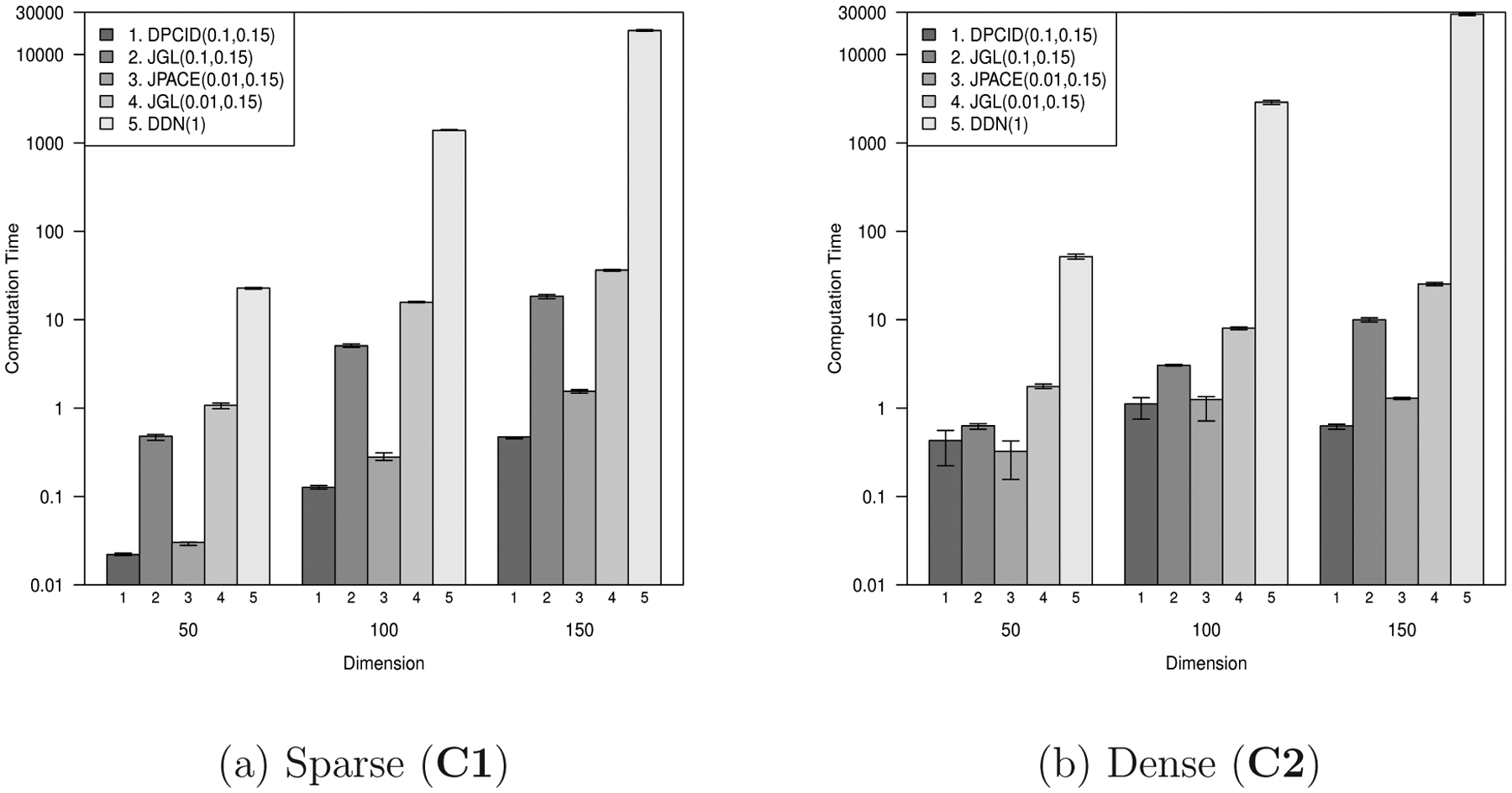
Comparison of computing times. In each panel, columns represent DPCID(0.01, 0.15), DPCID(0.1, 0.15), FGL(0.01, 0.15), FGL(0.1, 0.15), DDN(1), respectively. The numbers in parenthesis are tuning parameters (λ₁, λ₂) for DPCID and FGL and λ for DDN. The tuning parameters were chosen for the number of estimated differential edges to be similar.

Table 6:

Required memory spaces and complexity of algorithms for FGL, DDN, and DPCID. In the required memory space, we report the exact terms whose orders are greater or equal to p². The complexity of algorithms denotes the computational cost per iteration and are calculated from the implemented codes provided by authors.

Method	Required memory space	Complexity
FGL	13p2 + O(p)	O(p3)
DDN	$\frac{5}{4}{p}^4+\frac{1}{2}{p}^3+\frac{55}{4}{p}^2+O(p)$	$O\left({\left(\frac{p(p+1)}{2}\right)}^2\right)$
DPCID	10p2 + O((n1 + n2)p)	O(p3)

In summary, the DPCID is better than two other methods in view of AUC in all scenarios and its performance is stable in finding differential edges in view of four measures for classification accuracy. With consideration of computing time and memory requirements, the DPCID is favorable to the DDN, especially when p is large.

4. Application to Alzheimer’s Disease

We applied the DPCID to a real-world example of identifying differences in functional connectivity between patients with AD and HC. Based on the results of the numerical study, the BIC is the appropriate criterion to select the tuning parameter λ₂ since the brain networks has similar structure to the generated networks in (C2) rather than that in (C1). The dataset included 5.5-minute resting state fMRI scans from 29 HC with no history of head trauma, neurological disease or hearing disability and 33 patients who suffer from mild, moderate, or severe AD as determined by the National Institute of Neurological and Communicative Disorders and Stroke criteria [39]. RsfMRI data were collected with written consent and in accordance with institutional review at University of Medicine and Dentistry of New Jersey on a Bruker Medspec 3T 60-cm bore imaging system using a echo planar imaging sequence that was optimized for blood-oxygenation-level-dependent contrast (repetition time = 2000 ms; echo time = 25 ms; flip angle = 90; 39 slices, matrix = 64×64, FOV = 192 mm; acquisition voxel size = 3×3×3 mm; number of volumes = 115). Subjects were asked to rest with their eyes open while viewing the word “Relax”, which was centrally projected in white against a black background, during the scans.

All data sets from each of the subjects were processed in an identical fashion using AFNI (version AFNI_2008_07_18_1710, http://afni.nimh.nih.gov/afni; [40]) and FSL (version 3.3, www.fmrib.ox.ac.uk; [41]). Image preprocessing in AFNI consisted of slice time correction, motion correction, mean-based intensity normalization, spatial smoothing by 6mm FWHM Gaussian kernel, temporal high-pass and low-pass filtering, and correction for time series autocorrelation (pre-whitening). Functional data were then transformed into MNI152 space using a 12 degree of freedom linear affine transformation calculated using FSL’s FLIRT tool [42]. The functional data comprise a sequence of MRI. Each MRI consists of a number of voxels, the basic unit of volume element in MRI study. Thus, mean time series for each ROI (selection described below) were extracted from this standardized functional volume by averaging over all voxels within the region. To ensure that each time series represented regionally specific neural activity, the mean time series of each region of interest (ROI) was orthogonalized with respect to nine nuisance signals (global signal, white matter, cerebrospinal fluid, and six motion parameters).

In order to conduct an object survey of connectivity across the brain, while reducing the dimensionality of the resulting connectome graphs, graph nodes were chosen using 110 regions from the Harvard-Oxford (HO) structural atlas. HO is a probabilistic atlas that defines regions based on standard anatomical boundaries [43, 44]. A 25% threshold was applied to create a hard assignment for each region and the resulting map was bisected into left and right hemispheres at the mid line (x = 0). Regional time series, standardized to zero mean and unit variance, concatenated across individuals for each population. In this way, the number of sample increases and only one null precision matrix need to be estimated. The resulting time series were submitted to the DPCID to identify connectome graph differences between HC and AD populations.

Our method identified 59 connectome graph edges that differ between AD and HC (Table 7). Half of the identified connections are inter-hemispheric and the remaining differences are intra-hemispheric (Figures 4–5). The regions subtending the identified links are mostly associated with motor, memory, emotion processing and sensory brain systems - all of which make sense given symptoms typically associated with AD [45]. The brain stem appears to be a central locus of the disorder, as it is involved in several connections that differ between groups.

Table 7:

List of 59 connectome graph edges that differ between AD and HC. Edges are listed in decreasing order of absolute difference. L. and R. are acronyms of left and right, respectively.

L. Brain-Stem	R. Brain-Stem
L.Middle Temporal Gyrus, posterior division	R.Middle Temporal Gyrus, posterior division
R.Insular Cortex	R.Putamen
R.Insular Cortex	R.Pallidum
L. Brain-Stem	R.Thalamus
L.Superior Temporal Gyrus, anterior division	L.Middle Temporal Gyrus, temporooccipital part
L.Frontal Orbital Cortex	L.Temporal Fusiform Cortex, anterior division
R.Putamen	R.Pallidum
R.Pallidum	R. Brain-Stem
L.Parietal Operculum Cortex	R.Parietal Operculum Cortex
L.Parahippocampal Gyrus, posterior division	R.Parahippocampal Gyrus, anterior division
L. Caudate	R.Putamen
L.Inferior Frontal Gyrus, pars triangularis	L.Middle Temporal Gyrus, anterior division
L.FRONTAL POLE	L.Subcallosal Cortex
L.Inferior Temporal Gyrus, anterior division	L.Supramarginal Gyrus, posterior division
L.Temporal Occipital Fusiform Cortex	R.Inferior Temporal Gyrus, temporooccipital part
L. Brain-Stem	L.Accumbens
L.Supramarginal Gyrus, anterior division	R.Superior Parietal Lobule
L.Subcallosal Cortex	R.Occipital Pole
L.Inferior Temporal Gyrus, anterior division	R.Superior Temporal Gyrus, anterior division
R.Superior Frontal Gyrus	R.Putamen
L.Thalamus	R. Caudate
R.Superior Temporal Gyrus, posterior division	R.Inferior Temporal Gyrus, temporooccipital part
L.Parahippocampal Gyrus, posterior division	R. Brain-Stem
L.Planum Polare	R.Temporal Pole
L.Thalamus	R.Thalamus
R.Inferior Temporal Gyrus, anterior division	R.Temporal Fusiform Cortex, anterior division
L. Brain-Stem	R.Inferior Temporal Gyrus, posterior division
L.Middle Temporal Gyrus, anterior division	L.Inferior Temporal Gyrus, anterior division
L.Precuneous Cortex	L.Temporal Fusiform Cortex, posterior division
L. Brain-Stem	R.Superior Temporal Gyrus, posterior division
L.Temporal Pole	L.Temporal Fusiform Cortex, anterior division
L.Parahippocampal Gyrus, anterior division	L. Amygdala
R.Middle Temporal Gyrus, anterior division	R.Subcallosal Cortex
L.Parahippocampal Gyrus, anterior division	R.Parahippocampal Gyrus, anterior division
R.Frontal Medial Cortex	R.Frontal Orbital Cortex
R.Temporal Fusiform Cortex, anterior division	R.Thalamus
L.Inferior Temporal Gyrus, anterior division	L.Paracingulate Gyrus
L.Middle Temporal Gyrus, posterior division	L. Amygdala
L.Lingual Gyrus	R.Putamen
L.Insular Cortex	R.Superior Temporal Gyrus, anterior division
L.Central Opercular Cortex	R.Parietal Operculum Cortex
L.Juxtapositional Lobule Cortex	R.Putamen
L.Inferior Temporal Gyrus, temporooccipital part	R.Superior Temporal Gyrus, anterior division
L.Temporal Fusiform Cortex, anterior division	R. Hippocampus
R.Angular Gyrus	R.Lateral Occipital Cortex, superoir division
R.Middle Frontal Gyrus	R.Putamen
L.Paracingulate Gyrus	R.Putamen
L.Subcallosal Cortex	R.Subcallosal Cortex
L.Inferior Temporal Gyrus, anterior division	L.Juxtapositional Lobule Cortex
R.Temporal Fusiform Cortex, posterior division	R.Accumbens
R.Middle Frontal Gyrus	R.Precentral Gyrus
R.Precuneous Cortex	R.Putamen
L.Temporal Fusiform Cortex, anterior division	R.Middle Temporal Gyrus, anterior division
R.Precentral Gyrus	R.Inferior Temporal Gyrus, anterior division
R.Superior Temporal Gyrus, posterior division	R.Heschl’s Gyrus
L.Subcallosal Cortex	L. Hippocampus
L.Intracalcarine Cortex	R.Occipital Pole
R.FRONTAL POLE	R.Temporal Fusiform Cortex, anterior division

Figure 4:

Differential network between AD and HC in Axial view

Figure 5:

Differential network between AD and HC in medium view

5. Conclusions

In this paper, we proposed a penalized regression-based procedure to find differential edges between population-level partial correlation networks. We emphasize that sparsity is assumed only on the differences in the sense that two matrices differ from each other in a few elements, but not as a structural condition on the matrices of partial correlations. For this reason, the proposed method considers ℓ₂ penalty for elements of partial correlation matrices and ℓ₁ penalty for their differences. The proposed penalty is suitable for our motivational example of finding differences in brain functional connectivity between patients with AD and HC since we conjecture that connectome graphs are dense rather than sparse, but that the strength or degree of only a few connections in patients might differ. We developed a block-wise coordinate descent algorithm to solve the penalized regression problem and two tuning parameters are chosen by minimizing either the AIC (for sparse) or the BIC (for dense).

The DPCID has a couple of advantages over other existing methods. First, the sparse estimate of differences between two graphs of partial correlations is favorable for interpretation in practice. Second, the DPCID is more robust than other existing methods to standardization of observed variables in each condition since partial correlations are invariant under scaling, while all elements of each precision matrix would be affected by scaling operations. For instance, if we rescale each variable to have a unit variance, then the rescaled covariance matrix is $\tilde{\Sigma }=D^{-1/2}\Sigma D^{-1/2}$. In this case, the precision matrix is defined as $\tilde{\Omega }=D^{1/2}\Omega D^{1/2}=\left({\omega }_{ij}\sqrt{{\sigma }_{ii}{\sigma }_{jj}}\right)$, where $\Sigma ={\left({\sigma }_{ij}\right)}_{1\le i,j\le p}$ and $\Omega ={\left({\omega }_{ij}\right)}_{1\le i,j\le p}$ are the covariance and precision matrices before rescaling, respectively, and $D^{1/2}=\text{diag}\left(\sqrt{{\sigma }_{11}},\dots ,\sqrt{{\sigma }_{pp}}\right)$. These changes can cause unwanted differences in the precision matrices across all conditions.

Our simulation study suggests that our method is superior to the existing methods, the FGL and the DDN when networks are dense (see Tables 4–5).

Finally, we applied the proposed method to finding atypical functional connectivity in patients with AD based on rsfMRI. We find that 59 out of all possible 5,995 connections (around 0.98%) are different between HC and AD. Regions in brain of difference are mainly related to the functions of motor, memory and sensory.

References

- [1].Craddock RC et al. , Imaging human connectomes at the macroscale, Nature Methods 10 (2013), 524–539. [DOI] [PMC free article] [PubMed] [Google Scholar]
- [2].Varoquaux G and Craddock RC, Learning and comparing functional connectomes across subjects, Neuroimage 80 (2013), 405–415. [DOI] [PubMed] [Google Scholar]
- [3].Biswal B et al. , Functional connectivity in the motor cortex of resting human brain using echo-planar MRI, Magnetic Resonance in Medicine 34 (1995), 537–541. [DOI] [PubMed] [Google Scholar]
- [4].Shehzad Z et al. , The resting brain: Unconstrained yet reliable, Cerebral Cortex 19 (2009), 2209–2229. [DOI] [PMC free article] [PubMed] [Google Scholar]
- [5].Damoiseaux J et al. , Consistent resting-state networks across healthy subjects, Proceedings of the National Academy of Sciences of the United States of America 103 (2006), 13848–13853. [DOI] [PMC free article] [PubMed] [Google Scholar]
- [6].Yuan M and Lin Y, Model selection and estimation in the gaussian graphical model, Biometrika 94 (2007), 19–35. [Google Scholar]
- [7].Friedman J, Hastie T, and Tibshirani R, Sparse inverse covariance estimation with the graphical lasso, Biostatistics 9 (2008), 432–441. [DOI] [PMC free article] [PubMed] [Google Scholar]
- [8].Yuan M, High dimensional inverse covariance matrix estimation via linear programming, Journal of Machine Learning Research 11 (2010), 2261–2286. [Google Scholar]
- [9].Witten DM, Friedman JH, and Simon N, New insights and faster computations for the graphical lasso, Journal of Computational and Graphical Statistics 20 (2011), 892–900. [Google Scholar]
- [10].Mazumder R and Hastie T, The graphical lasso: New insights and alternatives, Electronic Journal of Statistics 6 (2012), 2125–2149. [DOI] [PMC free article] [PubMed] [Google Scholar]
- [11].Meinshausen N and Bühlmann P, High-dimensional graphs and variable selection with the lasso, The Annals of Statistics 34 (2006), 1436–1462. [Google Scholar]
- [12].Peng J et al. , Partial correlation estimation by joint sparse regression models, Journal of the American Statistical Association 104 (2009), 735–746. [DOI] [PMC free article] [PubMed] [Google Scholar]
- [13].Khare K, Oh S-Y, and Rajaratnam B, A convex pseudolikelihood framework for high dimensional partial correlation estimation with convergence guarantees, Journal of the Royal Statistical Society: Series B (Statistical Methodology) 77 (2015), 803–825. [Google Scholar]
- [14].Yu D et al. , Statistical completion of a partially identified graph with applications for the estimation of gene regulatory networks, Biostatistics 16 (2015), 670–685. [DOI] [PMC free article] [PubMed] [Google Scholar]
- [15].Ali A et al. , Generalized pseudolikelihood methods for inverse covariance estimation, Proceedings of Machine Learning Research 54 (2017), 280–288. [Google Scholar]
- [16].Cai TT, Liu WD, and Luo X, A constrained ℓ1 minimization approach to sparse precision matrix estimation, Journal of the American Statistical Association 106 (2011), 594–607. [Google Scholar]
- [17].Cai TT et al. , Covariate-adjusted precision matrix estimation with an application in genetical genomics, Biometrika 100 (2013), 139–156. [DOI] [PMC free article] [PubMed] [Google Scholar]
- [18].Cai TT, Liu W, and Zhou HH, Estimating sparse precision matrix: Optimal rates of convergence and adaptive estimation, The Annals of Statistics 44 (2016), 455–488. [Google Scholar]
- [19].Zou H and Hastie T, Regularization and variable selection via the elastic net, Journal of the Royal Statistical Society: Series B (Statistical Methodology) 67 (2005), 301–320. [Google Scholar]
- [20].Candes E and Tao T, The Dantzig selector: statistical estimation when p is much larger than n, The Annals of Statistics 35 (2007), 2313–2351. [Google Scholar]
- [21].Guo J et al. , Joint estimation of multiple graphical models, Biometrika 98 (2011), 1–15. [DOI] [PMC free article] [PubMed] [Google Scholar]
- [22].Mohan K et al. , Structured learning of gaussian graphical models, Advances in Neural Information Processing Systems 2012 (2012), 629–637. [PMC free article] [PubMed] [Google Scholar]
- [23].Mohan K et al. , Node-based learning of multiple gaussian graphical models, Journal of Machine Learning Research 15 (2014), 445–488. [PMC free article] [PubMed] [Google Scholar]
- [24].Danaher P, Wang P, and Witten DM, The joint graphical lasso for inverse covariance estimation across multiple classes, Journal of the Royal Statistical Society: Series B (Statistical Methodology) 76 (2014), 373–397. [DOI] [PMC free article] [PubMed] [Google Scholar]
- [25].Yang S et al. , Fused multiple graphical lasso, SIAM Journal on Optimization 25 (2015), 916–943. [Google Scholar]
- [26].Zhao SD, Cai TT, and Li H, Direct estimation of differential networks, Biometrika 101 (2014), 253–268. [DOI] [PMC free article] [PubMed] [Google Scholar]
- [27].Price BS, Geyer CJ, and Rothman AJ, Ridge fusion in statistical learning, Journal of Computational and Graphical Statistics 24 (2014), 439–454. [Google Scholar]
- [28].Yuan M and Lin Y, Model selection and estimation in regression with grouped variables, Journal of the Royal Statistical Society: Series B (Statistical Methodology) 68 (2006), 49–67. [Google Scholar]
- [29].Tibshirani R et al. , Sparsity and smoothness via the fused lasso, Journal of the Royal Statistical Society: Series B (Statistical Methodology) 67 (2005), 91–108. [Google Scholar]
- [30].van Wieringen WN and Peeters CFW, Ridge estimation of inverse covariance matrices from high-dimensional data, Computational Statistics & Data Analysis 103 (2016), 284–303. [Google Scholar]
- [31].Ryali S et al. , Estimation of functional connectivity in fMRI data using stability selection-based sparse partial correlation with elastic net penalty, Neuroimage 59 (2012), 3852–3861. [DOI] [PMC free article] [PubMed] [Google Scholar]
- [32].Boyd S, Distributed optimization and statistical learning via the alternating direction method of multipliers, Foundations and Trends in Machine Learning 3 (2010), 1–122. [Google Scholar]
- [33].Akaike H, A new look at the statistical model identification, IEEE Transactions on Automatic Control 19 (1974), 716–723. [Google Scholar]
- [34].Wolf M and Ledoit O, A well-conditioned estimator for large-dimensional covariance matrices, Journal of Multivariate Analysis 88 (2004), 365–411. [Google Scholar]
- [35].Tseng P, Convergence of a block coordinate descent method for nondifferentiable minimization, Journal of Optimization Theory and Applications 109 (2001), 475–494. [Google Scholar]
- [36].Prasad T et al. , Human protein reference database - 2009 update, Nucleic Acids Research 37 (2009), D767–772. [DOI] [PMC free article] [PubMed] [Google Scholar]
- [37].Watts D and Strogatz S, Collective dynamics of ‘small-world’ networks, Nature 393 (1998), 440–442. [DOI] [PubMed] [Google Scholar]
- [38].Eguíluz V et al. , Scale-free brain functional networks, Phyical Review Letters 94 (2005), 018102. [DOI] [PubMed] [Google Scholar]
- [39].McKhann G et al. , Clinical and pathological diagnosis of frontotemporal demetia: report of the work group on frontotoemporal dementia and pick’s disease, Archives of Neurology 58 (2001), 1803–1809. [DOI] [PubMed] [Google Scholar]
- [40].Cox R, AFNI: software for analysis and visualization of functional magnetic resonance neuroimages, Computers and Biomedical Research 29 (1996), 162–173. [DOI] [PubMed] [Google Scholar]
- [41].Jenkinson M et al. , FSL., Neuroimage 62 (2012), 782–790. [DOI] [PubMed] [Google Scholar]
- [42].Jenkinson M et al. , Improved optimization for the robust and accurate linear registration and motion correction of brain images, Neuroimage 17 (2002), 825–841. [DOI] [PubMed] [Google Scholar]
- [43].Kennedy D et al. , Gyri of the human neocortex: an MRI-based analysis of volume and variance, Cerebral Cortex 8 (1998), 372–384. [DOI] [PubMed] [Google Scholar]
- [44].Makris N et al. , MRI-based topographic parcellation of human cerebral white matter and nuclei II. rationale and applications with systematics of cerebral connectivity, Neuroimage 9 (1999), 18–45. [DOI] [PubMed] [Google Scholar]
- [45].Reiman E and Jagust W, Brain imaging in the study of Alzheimer’s disease, Neuroimage 61 (2012), 505–516. [DOI] [PMC free article] [PubMed] [Google Scholar]