Diverse coactive neurons encode stimulus-driven and stimulus-independent variables

Abstract

Both experimenter-controlled stimuli and stimulus-independent variables impact cortical neural activity. A major hurdle to understanding neural representation is distinguishing between qualitatively different causes of the fluctuating population activity. We applied an unsupervised low-rank tensor decomposition analysis to the recorded population activity in the visual cortex of awake mice in response to repeated presentations of naturalistic visual stimuli. We found that neurons covaried largely independently of individual neuron stimulus response reliability and thus encoded both stimulus-driven and stimulus-independent variables. Importantly, a neuron’s response reliability and the neuronal coactivation patterns substantially reorganized for different external visual inputs. Analysis of recurrent balanced neural network models revealed that both the stimulus specificity and the mixed encoding of qualitatively different variables can arise from clustered external inputs. These results establish that coactive neurons with diverse response reliability mediate a mixed representation of stimulus-driven and stimulus-independent variables in the visual cortex.

NEW & NOTEWORTHY V1 neurons covary largely independently of individual neuron’s response reliability. A single neuron’s response reliability imposes only a weak constraint on its encoding capabilities. Visual stimulus instructs a neuron’s reliability and coactivation pattern. Network models revealed using clustered external inputs.

INTRODUCTION

Neural variability is a key feature of neocortical neuronal responses. During repeated sensory stimulation, most neurons exhibit high trial-to-trial variability, whereas only a small number of neurons display reliable responses across trials (Softky and Koch 1993; Stringer et al. 2019a). Here, by “reliable responses,” we refer to neural responses that have similar temporal profiles across trials. The abundance of unreliable neurons in the cerebral cortex raises the question of to what extent these neurons contribute to the representation of stimulus-driven and stimulus-independent variables (Olshausen and Field 2006). Possible answers to this question arise from multiple sources. First, neural variability is correlated across neurons (Cohen and Kohn 2011) such that untuned/unreliable neurons enhance sensory information coding (Leavitt et al. 2017; Safaai et al. 2013). Second, the sensory cortex encodes not only stimuli but also behavioral variables (Dipoppa et al. 2018; McGinley et al. 2015; Niell and Stryker 2010; Stringer et al. 2019b; Vinck et al. 2015) or internal state variables (Allen et al. 2019; Vinck et al. 2015). Thus, neural response variability to sensory stimuli can be partially explained by experimentally observed stimulus-independent variables (Stringer et al. 2019b). These observations suggest that unreliable neurons may play a role in encoding both stimulus-driven and stimulus-independent unobserved variables.

There is a growing consensus in neuroscience that coactive ensembles of neurons, as opposed to single neurons, are the underpinning of cognition and behavior (Buzsáki 2010; Saxena and Cunningham 2019; Yuste 2015). How then do neurons in sensory cortex covary and encode stimulus-driven or stimulus-independent variables? We assume that single-trial neuronal responses consist of additive modulations of distinct latent factors. Furthermore, each latent factor is modulated by the gain specific to the neuron and the trial (Fig. 1A). The question of encoding stimulus-driven and stimulus-independent variables is usefully illustrated by considering the extreme ends of a spectrum of possibilities (Fig. 1B). At one extreme, reliable neurons covary and encode stimulus-driven variables, whereas unreliable neurons covary and encode stimulus-independent variables. At the other extreme, neurons covary and encode both stimulus-driven and stimulus-independent variables regardless of their reliability. Identifying where along this spectrum cortical encoding operates is fundamentally challenging because the stimulus-driven and the stimulus-independent variables are unobserved (Keemink and Machens 2019). These unobserved variables must be inferred from observed neuronal population activity, which, however, is highly variable across trials of repeated stimulus presentation. Supervised methods, such as demixed principal component analysis (Kobak et al. 2016) and targeted dimensionality reduction (Mante et al. 2013), can only partially solve this problem by inferring unobserved variables that are correlated to observed behavioral or task-related variables. A promising direction is to solve the problem by using unsupervised methods, as shown by recent works on the visual cortex (Stringer et al. 2019b) and the frontal cortex (Hirokawa et al. 2019). Here, we used an unsupervised method, tensor component analysis (TCA) (Williams et al. 2018), which allowed us to identify stimulus-driven and stimulus-independent unobserved variables in an unbiased fashion from observed neuronal population activity in response to repeated stimulus presentations.

Fig. 1.

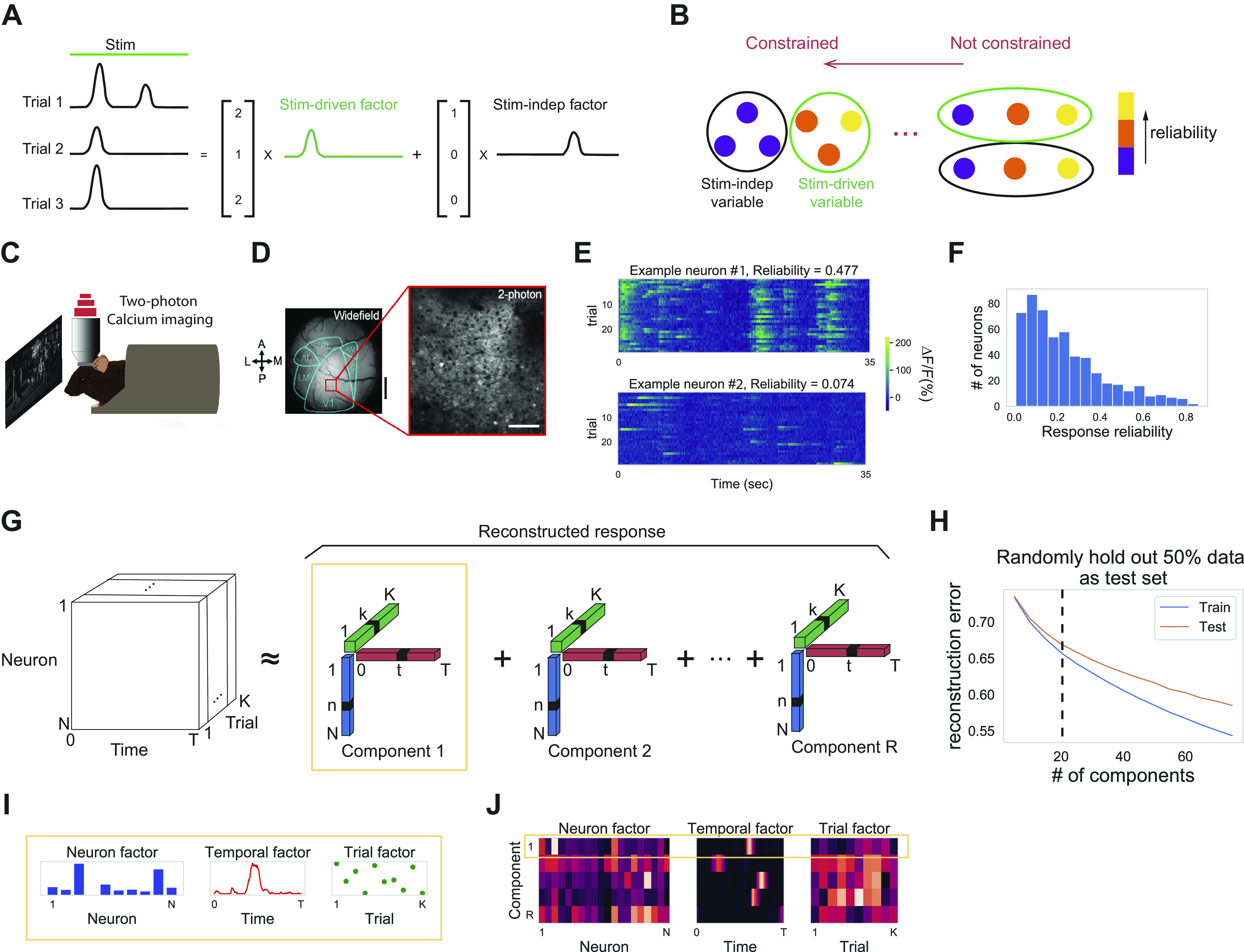
Response reliability has a skewed distribution. A: we decompose single trial neural responses into stimulus (Stim)-driven latent factors (green) that are consistent across trials and stimulus-independent (Stim-indep) latent factors (black) that are inconsistent across trials. B: schematic shows two extremes of a spectrum of possibilities for the encoding of stimulus-driven and stimulus-independent variables: left, reliable neurons covary and encode stimulus-driven variables, whereas unreliable neurons covary and encode stimulus-independent variables; right, neuron’s reliability does not constrain its encoding capability, and thus, neurons covary and encode both kinds of variables regardless of their reliability. C: experimental setup. We performed two-photon calcium imaging of excitatory neurons in the primary visual cortex of awake, head-fixed mice during visual stimulation with periodic drifting gratings and repeated identical naturalistic movie clips. D: visual cortex (contralateral to visual stimulus delivery) is retinotopically mapped in Emx1-Cre::TITL-GCaMP6s mice. V1 fields are chosen from the region selective for the center of the presentation screen. Widefield scale bar = 1 mm; two-photon scale bar = 100 μm. E: ∆F/F responses of one example neuron with high reliability (top) and one example neuron with low reliability (bottom) during the same naturalistic movie clip for 30 trials (movie starts at 5 s and lasts for 30-s duration). F: distribution of response reliability for 545 recorded neurons in one example imaging field. G: schematic of tensor component analysis (TCA). Neural data are organized into a third-order tensor with dimensions N × T × K (N denotes number of neurons, T represents number of time points in the trial, K represents number of trials). TCA approximates the data as a sum of outer products of three vectors from R components: neuron factors describe the weights of each neuron, temporal factors describe the temporal dynamics of each latent factor, and trial factors describe the modulation across trials. H: cross-validation of TCA (Williams et al. 2018) on one example data set (545 neurons × 350 frames × 30 trials). Cross-validated normalized reconstruction error (see methods) plotted against the number of components of TCA for training set (blue) and test set (orange). Dashed line denotes the TCA model with 20 components. I: one example component is displayed in the form of three vectors: neuron factor, temporal factor, and trial factor. J: all the components are displayed in the form of three heatmaps. Each row corresponds to one component (in this example R = 5).

We performed two-photon calcium imaging of excitatory neurons in the primary visual cortex of awake, head-fixed mice during visual stimulation with repeated identical naturalistic movie clips (Nat Mov) or periodic drifting gratings (PDG). We identified unobserved variables, or “latent factors,” representing either stimulus-driven variables or stimulus-independent variables. Our results show that neurons with a range of reliabilities covary and encode both stimulus-driven and stimulus-independent variables. Moreover, we found that the neuronal coactivation pattern is randomly redistributed across different stimuli. This suggests that feedforward inputs to neurons in the visual cortex have a significant influence on neuronal coactivation patterns. Finally, simulation of a neural network model revealed possible input structures underlying the observed encoding paradigm in the visual cortex.

MATERIALS AND METHODS

Lead Contact and Material Availability

Further information and requests for resources should be directed to and will be fulfilled by the lead contact, Ji Xia (xiaji@wustl.edu). We used tools for fitting TCA in https://github.com/ahwillia/tensortools.

Experimental Model and Subject Details

Animals.

For imaging visual cortical responses, a Emx1-Cre (Jax Stock #005628) × ROSA-LNL-tTA (Jax Stock #011008) × TITL-GCaMP6s (Jax Stock #024104) triple transgenic mouse line (n = 7) was bred to express GCaMP6s in cortical excitatory neurons (Madisen et al. 2015). Mice ranging in age from 6 to 20 wk of both sexes (3 males and 4 females) were implanted with a head plate and cranial window and imaged starting >2 wk after recovery from surgical procedures and up to 10 mo after window implantation. The animals were housed on a 12-h light/dark cycle in cages of up to five animals before the implants and individually after the implants. All animal procedures were approved by the Institutional Animal Care and Use Committee at University of California, Santa Barbara.

Surgical procedures.

All surgeries were conducted under isoflurane anesthesia (3.5% induction, 1.5%–2.5% maintenance). Prior to incision, the scalp was infiltrated with lidocaine (5 mg/kg, sc) for analgesia, and meloxicam (1 mg/kg, sc) was administered preoperatively to reduce inflammation. Once anesthetized, the scalp overlying the dorsal skull was sanitized and removed. The periosteum was removed with a scalpel, and the skull was abraded with a drill burr to improve adhesion of dental acrylic. A 4-mm craniotomy was made over the visual cortex (centered at 4.0 mm posterior, 2.5 mm lateral to bregma), leaving the dura intact. A cranial window was implanted over the craniotomy and sealed first with silicon elastomer (Kwik-Sil, World Precision Instruments) and then with dental acrylic (C&B-Metabond, Parkell) mixed with black ink to reduce light transmission. The cranial windows were made of two rounded pieces of coverglass (Warner Instruments) bonded with a UV-cured optical adhesive (Norland, NOA61). The bottom coverglass (4 mm) fit tightly inside the craniotomy, whereas the top coverglass (5 mm) was bonded to the skull using dental acrylic. A custom-designed stainless-steel head plate (eMachineShop.com) was then affixed using dental acrylic. After surgery, mice were administered carprofen (5–10 mg/kg, oral) every 24 h for 3 days to reduce inflammation. The full specifications and designs for head fixation hardware can be found on the Goard laboratory website (https://goard.mcdb.ucsb.edu/resources).

Two-photon imaging.

After >2 wk of recovery from surgery, GCaMP6s fluorescence was imaged using a Prairie Investigator 2-photon microscopy system with a resonant galvo scanning module (Bruker). For fluorescence excitation, we used a Ti:Sapphire laser (Mai-Tai eHP, Newport) with dispersion compensation (Deep See, Newport) tuned to λ = 920 nm. For collection, we used GaAsP photomultiplier tubes (PMTs; Hamamatsu). We used a ×16/0.8 NA microscope objective (Nikon) at ×1 or ×2 magnification, obtaining a square field of view with width ranging from 414 to 828 μm. Laser power ranged from 40 to 75 mW at the sample depending on GCaMP6s expression levels. Photobleaching was minimal (<1%/min) for all laser powers used. A custom-made stainless-steel light blocker (https://goard.mcdb.ucsb.edu/resources) was mounted to the head plate and interlocked with a tube around the objective to prevent light from the visual stimulus monitor from reaching the PMTs. During imaging experiments, the polypropylene tube supporting the mouse was suspended from the behavior platform with high-tension springs to reduce movement artifacts.

Two-photon postprocessing.

Images were acquired using PrairieView acquisition software and converted into TIF files. All subsequent analyses were performed in MATLAB (MathWorks) using custom code (https://goard.mcdb.ucsb.edu/resources). First, images were corrected for X-Y movement by registration to a reference image (the pixel-wise mean of all frames) using two-dimensional cross-correlation.

To identify responsive neural somata, a pixel-wise activity map was calculated using a modified kurtosis measure. Neuron cell bodies were identified using local adaptive threshold and iterative segmentation. Automatically defined regions of interest (ROIs) were then manually checked for proper segmentation in a graphical user interface (allowing comparison with raw fluorescence and activity map images). To ensure that the response of individual neurons was not due to local neuropil contamination of somatic signals, a corrected fluorescence measure was estimated according to:

$$F_{corrected }\left(n\right)=F_{soma}\left(n\right)-\alpha *F_{neuropil}\left(n\right)$$

where F_neuropil was defined as the fluorescence in the region <30 μm from the ROI border (excluding other ROIs) for frame n and α was chosen from [0, 1] to minimize the Pearson’s correlation coefficient between F_corrected and F_neuropil. The ∆F/F for each neuron was then calculated as:

$$\Delta F/F=\left(F_n-F_0\right)/F_0$$

where F_n is the corrected fluorescence (F_corrected) for frame n and F₀ defined as the mode of the corrected fluorescence density distribution across the entire time series. We calculated ∆F/F over windows of 500 samples (50 s). Since the threshold for nonstationarity is <1%/min across for the recording, this window adequately accounts for any small baseline drift.

Visual stimuli.

All visual stimuli were generated with a Windows PC using MATLAB and the Psychophysics toolbox (Brainard 1997). Stimuli used for two-photon imaging were presented on an LCD monitor (17.5 × 13 cm, 800 × 600 pixels, 60 Hz refresh rate) positioned 5 cm from the eye at a horizontal tilt of 30° to the right of the midline and vertical tilt of 18° downward, spanning 120° (azimuth) by 100° (elevation) of visual space in the right eye.

For drifting grating visual stimulation, 12 full-contrast sine wave gratings (spatial frequency: 0.05 cycles/°; temporal frequency: 2 Hz) were presented full-field, ranging from 0° to 330° in 30° increments. We presented eight repeats of the drifting grating stimulus; a single repeat of stimulus consisted of all 12 grating directions presented in order for 2 s with a 4-s interstimulus interval (gray screen).

For natural movie visual stimulation, we displayed a grayscale 30-s clip from Touch of Evil (Orson Wells, Universal Pictures, 1958) containing a continuous visual scene with no cuts (https://observatory.brain-map.org/visualcoding/stimulus/natural_movies). The clip was contrast-normalized and presented at 30 frames per second. We presented 30 repeats of the natural movie stimulus; each repeat started with 5 s of gray screen, followed by the 30 s of movie.

When we compared neural responses across stimuli, we did analyses on part of the responses so that their trial structure matches. For Nat Mov, we took the first 240 time points after movie onset and the first eight trials of the responses. For PDG, we took concatenated neural responses during PDG without the gray screen periods to get 240 time points (20 time points × 12 orientations). Thus, two types of neural responses would have the same trial structure (240 time points × 8 trials).

Nonnegative tensor decomposition with missing data.

We organized our data into a three-way tensor χ (N × T × K), and let χ_ntk represent the activity of neuron n at time t and trial k. Nonnegative tensor component analysis (TCA) decomposes χ into a sum of R rank-one tensors, where each rank-one tensor can be written as an outer product of three nonnegative vectors:

$$x_{ntk}\approx {{\displaystyle \sum }}_{r=1}^R{w}_b^r{b}_t^r{a}_k^t={\widehat{x}}_{ntk}$$

Nonnegative TCA with missing values was fit to minimize the squared reconstruction error:

$${\left|\right|M*\left(\chi -\widehat{\chi }\right)\left|\right|}_F^2$$

while

$$W\ge 0,B\ge 0,A\ge 0$$

Here, $\widehat{\chi }$ denotes the reconstructed data. ${\left|\right|\cdot \left|\right|}_F^2$ denotes the squared Frobenius norm of a tensor:

$${\left|\right|\chi \left|\right|}_F^2={{\displaystyle \sum }}_{n=1}^N{{\displaystyle \sum }}_{t=1}^T{{\displaystyle \sum }}_{k=1}^K{x}_{ntk}^2$$

where M denotes a masking tensor with the same shape as χ, and $*$ denotes entrywise multiplication of two tensors. For fitting nonnegative TCA on ∆F/F data, we set m_ntk = 0 if χ_ntk < 0; otherwise, we set m_ntk = 1. Normalized reconstruction error is the squared reconstruction error normalized by ${\left|\left|M*\chi \right|\right|}_F^2$.

Different from matrix decompositions, tensor decompositions are often unique (Kruskal 1977). However, when R is large or W, B, A have a low rank, it could be difficult to optimize. To monitor this possibility, we calculated similarity between different TCA fitting results on the same data set as described in the article by Williams et al. (2018). We found that the similarity between fitting results is close to 1 for all the nonnegative TCA models reported in this work.

Preprocessing of ∆F/F data.

∆F/F data were normalized such that the averaged squared sum of ∆F/F traces over time equals to 1 for every neuron:

$$\sqrt{\left({{\displaystyle \sum }}_{tk}^{}{x}_{ntk}^2\right)/TK}=1$$

This normalization step is crucial for ensuring TCA fitting is not biased by high firing rate neurons, since TCA is optimized to minimize the squared reconstruction error.

Choice of the number of components in TCA.

We picked the number of TCA components such that they captured a significant amount of neural responses without overfitting, checked with cross-validation as previously reported (Williams et al. 2018). To perform cross-validation, we randomly masked out 50% of tensor entries in χ. The remaining data were training set, and the masked-out data were test set. We trained nonnegative TCA with missing values to fit the training set. And then we used the trained TCA model to fit the test set. As we increase the number of components in TCA, if the normalized reconstruction error of the test set went up, the TCA model would overfit the training set. As previously reported (Williams et al. 2018), TCA is unlikely to overfit, even with up to 60 components. For this study, we chose 20 components for TCA, given that 20-component TCA captured a significant amount of neural responses without overfitting. Note that all the results in this study were robust to changes in the number of TCA components (data not shown; we tested TCA with 10–40 components).

Balanced network model.

Neurons were modeled as binary units. We simulated 1,600 excitatory neurons and 400 inhibitory neurons. The spiking $s_i^x$ of neuron i in population x ∈ {E,I} was given by

$$s_i^x\left(t\right)=\Theta \left({{\displaystyle \sum }}_{j=1}^{2000}{J}_{ij}{s}_j+{\mu }^x+{{\displaystyle \sum }}_{m=1}^{20}{g}_m\times K_{im}\times {\eta }_m+{{\displaystyle \sum }}_{n=1}^{20}{L}_{in}\times {\xi }_n-{\theta }^x\right)$$

where Θ is the Heaviside step function. J_ij is the connectivity weight from neuron j to neuron i. Each neuron received, on average, 200 excitatory and 200 inhibitory recurrent inputs, thus most matrix elements J_ij were zero. For the nonzero matrix elements J_ij, the synaptic weights were J^EE = J^IE = 0.07; J^EI = −0.14; J^II = −0.13. Bias current was given by µ^E = 1.13; µ^I = 0.91. Spiking threshold was given by θ^E = 1; θ^I = 0.7. Choices of parameters are motivated by previous work in the balanced network (Litwin-Kumar and Doiron 2012; van Vreeswijk and Sompolinsky 1998).

Frozen input pulse trains η consisted of 20 pulse trains repeated over trials, thus imitating the stimulus-driven variables (Supplemental Fig. S4D; all Supplemental material is available at https://doi.org/10.6084/m9.figshare.12885005). On each trial, each frozen pulse train contained one burst of three pulses during a random located time window of 200 ms (Supplemental Fig. S4D). Another set of 20 different input pulse trains ξ varied across trials, thus imitating stimulus-independent variables (Supplemental Fig. S4E). Since stimulus-independent variables are not locked to the trial structure, we generated trial-varied input pulse trains as Poisson pulse trains with a rate of 0.005 Hz during 500 s, i.e., the duration of the simulation.

K is a 2,000 × 20 matrix, describing synaptic weights between frozen input pulse trains and individual neurons. Each neuron only received one frozen pulse train, and each frozen pulse train innervated 100 neurons. The nonzero entries of K followed a lognormal distribution with mean = 2 (Supplemental Fig. S4B https://doi.org/10.6084/m9.figshare.12885005). g is a constant gain factor varying from trial to trial, randomly selected from a uniform distribution U (0.3, 0.8). L is a 2,000 × 20 matrix, describing synaptic weights between trial-varied input pulse trains and individual neurons. Each neuron only received one trial-varied pulse train, and each trial-varied pulse train innervated 100 neurons. Similar to K, the nonzero entries of L followed a lognormal distribution (Supplemental Fig. S4B https://doi.org/10.6084/m9.figshare.12885005). Both (1) the burst-like temporal structure of the input pulse trains and (2) the clusters of neurons with identical input pulse trains were chosen to impose a level of coordinated spiking within the otherwise unstructured recurrent model neural network.

To simulate neural responses to two different stimuli, we generated two sets of frozen input pulse trains and trial-varied input pulse trains as well as the corresponding input synaptic weights independently with the same statistics as described above.

Simulations were performed with a discrete time step of 10 ms, and neurons are updated asynchronously with a fixed order. At the beginning of each trial, 20% of neurons were randomly selected to be active, with the rest of neurons being silent. We simulated 20 trials for each stimulus. Each trial was simulated for 25 s. We convolved the simulated spike train with a kernel e^−t/τ₂ − e^−t/τ₁ similar to GCaMP6s kernel to generate simulated ∆F/F traces (rise time τ₁ = 100 ms, decay time τ₂ = 2 s). TCA was fitted on subsampled simulated ∆F/F traces with a time resolution of 100 ms.

Quantification and Statistical Analysis

Correlation between reliability of coactive neuron pairs.

To investigate dependency on reliability for neuronal coactivation, we calculated the Pearson correlation between reliability of significantly positively correlated neuron pairs in all recorded imaging fields. To select those neuron pairs, we calculated the Pearson correlation between pairs of neuronal responses and picked neuron pairs with positive and significant (P < 0.001) correlations.

Ordering of TCA components.

For analysis on responses during Nat Mov, TCA components were ordered by their consistency over trials. The consistency of TCA components was quantified as coefficient of variation (CV) of their trial factors.

For analysis on concatenated responses, TCA components were first separated into two groups based on whether the sum of trial factors during first eight trials (during PDG stimulation) was higher than sum of trial factors during second eight trials (during Nat Mov stimulation). Then, within each group, TCA components were ordered by their consistency.

Sorting neurons by dominant components.

Neurons were reordered by their dominant components. There were two steps for this sorting method. First, we grouped neurons by their dominant component. Dominant component was defined as the component with the highest neuron factor value for a given neuron. Second, within each group of neurons with the same dominant component, we sorted neurons by their neuron factor values of the dominant component in descending order.

Fitting performance.

We used the coefficient of determination (R²) to quantify the fitting performance of reconstructed responses by TCA components. Before we calculated R² between normalized ∆F/F traces and reconstructed ∆F/F traces, we set the negative part of normalized ∆F/F and corresponding part of reconstructed ∆F/F traces to zero.

Response reliability.

Response reliability was defined as the correlation coefficient of neural responses between pairs of trials averaged over all trial pairs for a given neuron:

$$Reliabilit{y}_i = \frac{2}{K\left(K-1\right)}{{\displaystyle \sum }}_{k_1=1}^K{{\displaystyle \sum }}_{k_2=k_1+1}^K\frac{Cov\left(r_{k_1}, r_{k_2}\right)}{\sqrt{Var\left(r_{k_1}\right) Var\left(r_{k_2}\right)}}$$

RESULTS

Response Reliability Has a Skewed Distribution

We recorded from layer 2/3 pyramidal neurons in V1 of awake, head-fixed mice using two-photon calcium imaging of transgenic mice expressing the calcium indicator GCaMP6s in excitatory neurons (see methods) (Fig. 1, C and D; Supplemental Fig. S1A https://doi.org/10.6084/m9.figshare.12885005). Mice watched a repeated clip of a 30-s naturalistic movie for 30 trials while being constrained within a tube (see methods). We recorded from 10 imaging fields in seven mice and extracted calcium responses (∆F/F) from a total of 4,077 well-isolated somatic regions of interest (ROIs). Numbers of ROIs from individual imaging fields were 545, 449, 791, 366, 480, 127, 284, 306, 371, and 358. Neuronal responses varied across trials. Using previously described methods (Goard and Dan 2009; Rikhye and Sur 2015), we quantified this response variation in terms of the “response reliability,” defined as the correlation coefficient of neural responses between pairs of trials averaged over all trial pairs for a given neuron (Fig. 1E; see methods). Response reliability distributions were skewed, with most neurons exhibiting low response reliability (Fig. 1F; Supplemental Fig. S1B https://doi.org/10.6084/m9.figshare.12885005). Note that the skewed distribution was not a result from the slow dynamics of calcium transients (Supplemental Fig. S1C https://doi.org/10.6084/m9.figshare.12885005). Because of the unimodal distribution, a distinction between “reliable” and “unreliable” neurons is not useful.

Neurons Covary Significantly with Each Other during Stimulus Presentation

To quantify the level of coordination among the neurons in the population activity, we applied nonnegative TCA (see methods) to the normalized ∆F/F data from recordings organized into a three-dimensional tensor (Fig. 1, G–J), as previously described (Williams et al. 2018). Single neuronal ∆F/F response was normalized by a constant so that its L2 norm equaled 1 (see methods). We found that with 20 components, the nonnegative TCA decomposition captured a significant amount of neural responses (545 neurons × 350 time points × 30 trials) for neurons with diverse reliability without overfitting (Figs. 1H and 2A). We quantified the fitting performance of individual neurons by the coefficient of determination (R²) and found that, in general, fitting performances on neurons with high reliability were higher than that of neurons with low reliability (Fig. 2B). Given that TCA is built to capture responses that are shared across dimensions (across neurons, time, or trials), it is not surprising to see that neurons with high reliability, whose responses are shared across trials, were better fit. However, for some neurons with low reliability, fitting performances were also surprisingly high (Fig. 2B), which suggests that their responses are shared across neurons. To quantify the extent to which neuronal responses are shared across neurons, we fitted TCA on neural responses with randomly shuffled trials for each neuron independently. Note that the reliability of each neuron after shuffling is still the same as that in the original data. Fitting performances on the original data were significantly better than fitting performances on data with shuffled trials (Fig. 2C), especially for neurons with low reliability. Furthermore, neurons were coactive largely independent of their reliability, supported by weak correlation between reliability of coactive neuron pairs (Supplemental Fig. S2D https://doi.org/10.6084/m9.figshare.12885005, see methods). In conclusion, this comparison indicates that neuronal coactivation pattern significantly contributes to population activity during stimulus presentation from single (Fig. 2C) and combined experiments (Supplemental Fig. S2, B and C https://doi.org/10.6084/m9.figshare.12885005).

Fig. 2.

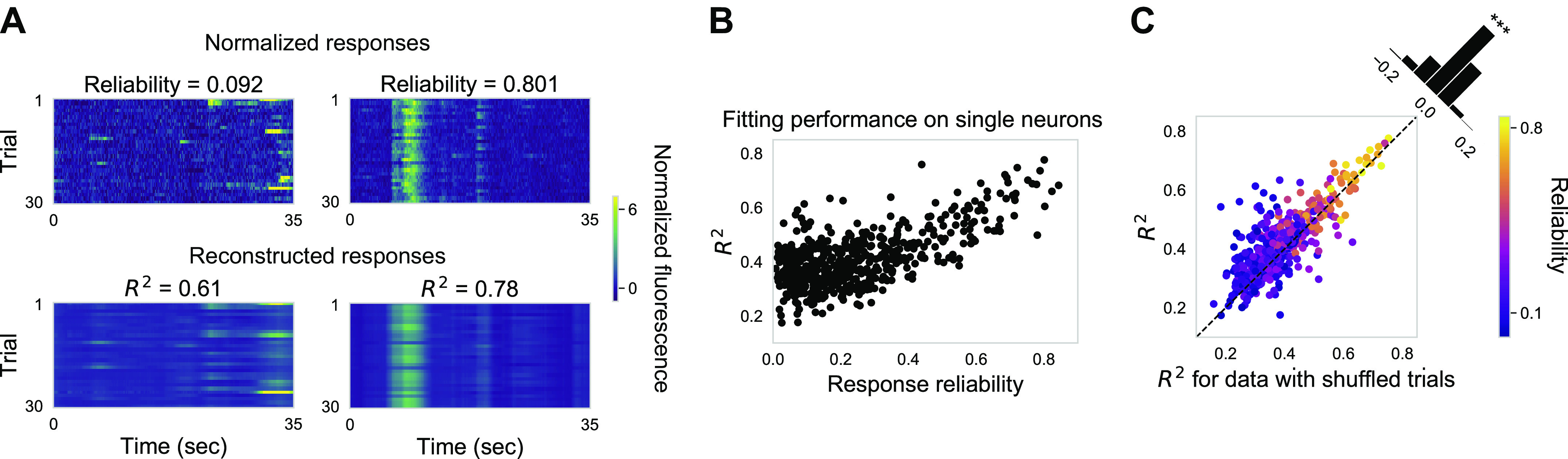
Neurons covary significantly with each other during stimulus presentation. A: ∆F/F traces (top) and reconstructed ∆F/F traces (bottom) based on 20 TCA components for one example neuron with low reliability (left) and one example neuron with high reliability (right) across trials in one example imaging field. B: fitting performance R² plotted against response reliability. Each dot represents one neuron in the example imaging field. C: fitting performance R² for original data plotted against R² for data with shuffled trials. Each dot represents one neuron. Color indicates response reliability. Fitting performance for the original data is significantly better than for data with shuffled trials (Mann–Whitney rank test, P < 0.001) in the same imaging field as in A and B. TCA, tensor component analysis.

Neurons with a Range of Reliabilities Are Coactive and Encode Stimulus-Driven and Stimulus-Independent Variables

To reveal the encoding paradigm of the neurons, we visualized all 20 TCA components in matrix form, sorted by their consistency across trials (Fig. 3A). Here, neuron factors directly reflect the coactivation pattern of the neurons (Supplemental Fig. S2, E and F https://doi.org/10.6084/m9.figshare.12885005), and trial factors indicate whether the TCA components are driven by the stimulus. We quantified the consistency of components by the coefficient of variation (CV) of their trial factors. Consistent components with low CV represent stimulus-driven variables, whereas inconsistent components with high CV represent stimulus-independent variables. In addition, we sorted the neurons based on their response reliability when visualizing neuron factors. The sorting by consistency and reliability revealed two key observations. First, there is a continuous distribution of consistency of components. Second, neurons with diverse reliability covary and encode different components, as indicated by 10 neurons with the highest neuron factor values for each component spanning a range of reliabilities (Fig. 3B). In other words, a single neuron’s response reliability imposes only a weak constraint on its encoding capabilities. This spread of coactivation pattern across reliability leads to a seemingly paradoxical conclusion that neurons with low reliability can encode stimulus-driven variables and neurons with high reliability can encode stimulus-independent variables (Supplemental Fig. S2, G and H https://doi.org/10.6084/m9.figshare.12885005). This apparent paradox is illustrated by responses from two example neurons (Fig. 3, C and D). The neuron with low reliability in Fig. 3C displayed highly variable responses from trial to trial; however, whenever it fired, it fired at the same time point in the trial. Thus, the neuron with low reliability had a high neuron factor value (higher than 1 SD above mean) for the consistent component shown in Fig. 3C. By contrast, the neuron with high reliability in Fig. 3D had a high neuron factor value for the corresponding inconsistent component. This resulted from the fact that the neuron with high reliability encoded not only stimulus-driven variables but also stimulus-independent variables. The findings indicate that one neuron can covary with different groups of neurons and can encode distinct variables. The two key observations hold for all the recorded imaging fields (Supplemental Fig. S3 https://doi.org/10.6084/m9.figshare.12885005; Fig. 4). In other words, a single neuron’s response reliability imposes only a weak constraint on its encoding capabilities with natural movie stimulation. In addition, the two key observations largely hold for neural responses to drifting gratings; however, there were fewer neurons with high reliability encoding stimulus-independent variables (Supplemental Fig. S3 https://doi.org/10.6084/m9.figshare.12885005).

Fig. 3.

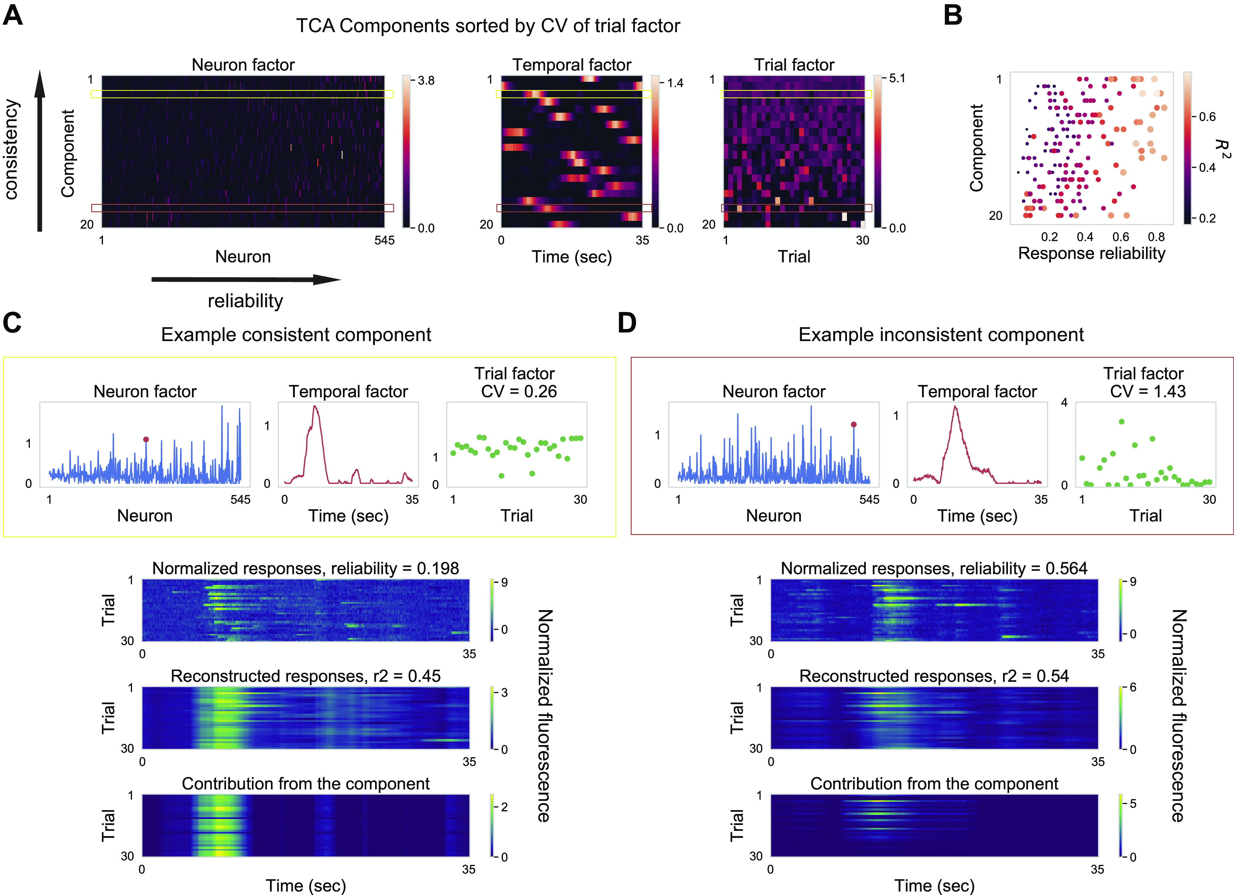
Neurons with a range of reliabilities are coactive and encode stimulus-driven and stimulus-independent variables. A: neuron, temporal, and trial factors of nonnegative TCA with 20 components. For all three factors, components are ordered by coefficient of variation (CV) of trial factors. In addition, within the neuron factors, neurons are ordered by their response reliability. Two example components are highlighted by horizontal rectangles: (yellow) A “consistent” component with a low CV value of trial factors. (red) An “inconsistent” component with a high CV value of trial factors. Color scale units are arbitrary units. B: reliability (abscissa) and R² values (color and dot diameter) for the top 10 neurons with the largest neuron factor values within a component, shown for all 20 components (ordinate). Components are in the same order as in A. C: one example component (same as yellow rectangle in D) that is consistent across trials (trial factor has low CV value). For clarity, here we used the display format of factors as described in Fig. 1I. For one neuron (red dot), the normalized responses and the reconstructed responses are shown below. As seen from the reconstructed response using this component alone (bottom), this neuron with low reliability has a large contribution from the consistent component. D: one example component (same as red rectangle in D) that is inconsistent across trials (trial factor has high CV value). For one neuron (red dot), the normalized responses and the reconstructed responses are shown below. As seen from the reconstructed response using this component alone (bottom), this neuron with high reliability has a large contribution from the inconsistent component. TCA, tensor component analysis.

Fig. 4.

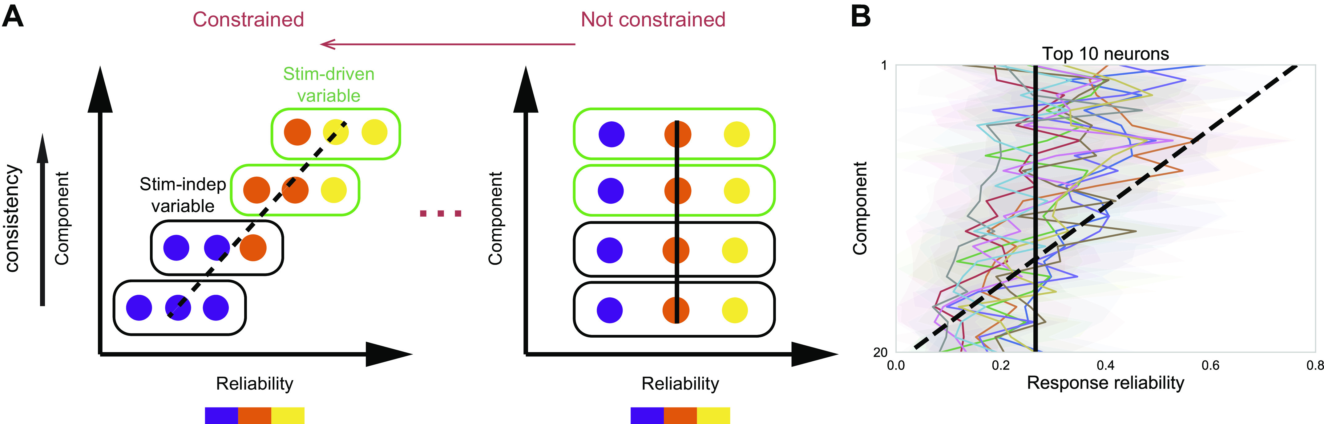
A single neuron’s response reliability imposes only a weak constraint on its encoding capabilities. A: schematic shows reliability distribution of neurons encoding stimulus (Stim)-driven and stimulus-independent (Stim-indep) variables for extremes of a spectrum of possibilities illustrated in Fig. 1B. Reliability of neurons with large neuron factor values is shown for each TCA component. Consistent components are assumed to represent stimulus-driven variables, whereas inconsistent components are assumed to represent stimulus-independent variables. Left: neuron’s encoding capability is constrained by its reliability; right: neuron’s encoding capability is not constrained by its reliability. B: reliability (abscissa) averaged over top 10 neurons with the largest neuron factor values within a component, shown for all 20 components (ordinate). Components are ordered by consistency, similar to Fig. 3B. Shaded area denotes standard deviation of reliability over the top 10 neurons. Here, different colors denote different imaging fields. Reliability is positively correlated with the consistency of components (10 imaging fields; Spearman’s correlation r = 0.37 ± 0.093, P < 0.05). Dashed line denotes the expected relation between reliability and the consistency of components under constrained extreme, whereas solid line denotes the expected relation under unconstrained extreme. TCA, tensor component analysis.

Neuronal Coactivation Pattern Randomly Redistributes across Different Stimuli

Cortical neurons are deeply embedded in a recurrent neural circuit (Douglas et al. 1995). The recurrent nature of cortical circuits raises the question of how the observed single-neuron reliability and the population coactivation patterns are modulated by feedforward visual input. To investigate the impact of feedforward and recurrent input, we analyzed neural responses to a naturalistic movie clip (Nat Mov) and periodic drifting gratings (PDG) stimuli from neurons in the same imaging field. To make a direct comparison across stimuli, we matched their trial structure for all analyses (see methods).

First, we compared how single neuron activity changes across stimuli. The activity level (averaged ∆F/F over time) of cortical neurons followed a skewed distribution during both Nat Mov and PDG stimulation (Fig. 5A). In addition, neurons’ activity level substantially redistributed across stimuli (Fig. 5B). The response reliability to both stimuli also followed skewed distributions (Fig. 5C) and extensively redistributed across stimuli (Fig. 5D).

Fig. 5.

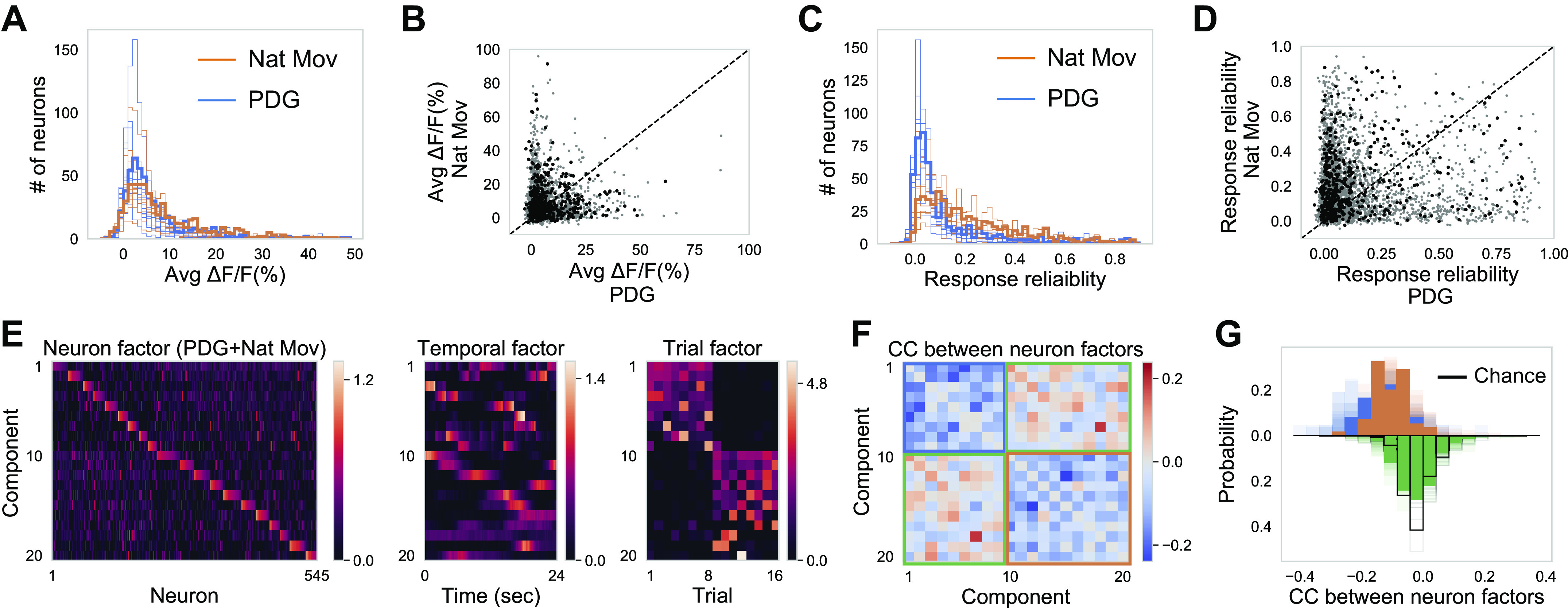
Neuronal coactivation pattern randomly redistributes across different stimuli. A: distribution of averaged ∆F/F (%) over time and trials during Nat Mov and PDG for one imaging field (opaque color) and the other nine imaging fields (transparent color). B: averaged (Avg) ∆F/F (%) during Nat Mov plotted against averaged ∆F/F (%) during PDG for neurons in one imaging field (black dots) and neurons in the other nine imaging fields (gray dots). Averaged ∆F/F (%) during Nat Mov is weakly correlated with averaged ∆F/F (%) during PDG (4,077 neurons, Pearson’s correlation r = 0.07, P < 0.001). C and D: same as A and B, but for response reliability. Reliability during Nat Mov is weakly correlated with reliability during PDG (4,077 neurons, Pearson’s correlation r = 0.09, P < 0.001). E: 20 TCA components for concatenated neural responses to visual stimulation with PDG and Nat Mov. Ordering of components is determined by their trial factors (see methods). Neuron factors are plotted with neurons ordered by their dominant components (see methods). F: the correlation coefficient (CC) between neuron factors are displayed with the same component order as in E (diagonal entries are set to zero). G: distribution of CC between neuron factors. Orange is for CC between neuron factors during Nat Mov; blue is for CC between neuron factors during PDG; green is for CC between neuron factors across stimuli; black is for CC between random vectors with the same dimension as neuron factors, representing the chance level. Opaque color is for one imaging field; transparent color is for the other nine imaging fields. Both CC during Nat Mov and CC during PDG are significantly negative (one-sample t test, for all 10 imaging fields, P < 0.001). CC across stimuli is centered around zeros (one-sample t test, for all 10 imaging fields, P > 0.1). Nat Mov, naturalistic movie clips; PDG, periodic drifting grating; TCA, tensor component analysis.

Second, we compared how neuronal ensembles change across stimuli. Are neurons coactive in the same way during Nat Mov stimulation and PDG stimulation? To answer this question, we fitted TCA with 20 components on concatenated neural responses (Fig. 5E). Note that TCA is ignorant to which stimulus is on during each trial. Despite this lack of information about the trial structure, TCA successfully identified two groups of components corresponding to the two stimuli (Fig. 5E). As expected, the consistent components during PDG stimulation reflect the tuning curves of orientation selective neurons, with two peaks for their temporal factors corresponding to responses to orientations separated by 180°. To quantify similarities between neural ensembles, we calculated the correlation coefficient (CC) between neuron factors of different components (Fig. 5F). Note that TCA factors are not necessarily orthogonal to each other, in contrast to principal component analysis (Kruskal 1977; Williams et al. 2018). Thus, the CC between neuron factors is not expected to be zero or negative. We found that intercomponent CCs within stimuli were predominantly negative, whereas intercomponent CCs across stimuli centered around zero (Fig. 5G). A negative CC between two components indicates that if one neuron is recruited by one component, it is unlikely to be recruited by the other component. Consequently, different TCA components within stimuli, i.e., Nat Mov or PDG, tend to be encoded by largely nonoverlapped ensembles of neurons, whereas different TCA components across stimuli, i.e., Nat Mov versus PDG, tend to be encoded by random ensembles of neurons. Importantly, the fact that neuronal ensembles are randomly reorganized for different external visual inputs raises the question of whether neural ensembles are formed mainly due to feedforward external inputs instead of cortical recurrent connections.

A Balanced Model Network with Random Connectivity and Correlated External Inputs Reproduces Key Features of the Observed Cortical Activity

To identify a potential mechanism behind the observed cortical dynamics, we simulated a balanced model network (van Vreeswijk and Sompolinsky 1996, 1998) with random connectivity and clustered external inputs (clustered as defined by grouping of neuron inputs; note that the model has no spatial organization, see methods and Fig. 6A). In brief, the recurrent model network consisted of 1,600 excitatory and 400 inhibitory binary point neurons with uniform random connectivity for each neuron type (see Supplemental Fig. S4A https://doi.org/10.6084/m9.figshare.12885005 and methods). To mimic stimulus-driven and stimulus-independent variables in the model, we constructed two qualitatively different sets of external input pulse trains (Supplemental Fig. S4, D and E https://doi.org/10.6084/m9.figshare.12885005). One set of 20 different input pulse trains was identical (“frozen”) across trials, thus imitating stimulus-driven variables. Another set of 20 different input pulse trains varied in a trial-independent manner, thus imitating stimulus-independent variables. To mimic coactivation patterns among neurons, we randomly partitioned the 2,000 model neurons into 20 clusters of 100 model neurons each. All neurons within a cluster received the same “frozen” input pulse train. For another random partitioning of the model neurons into 20 clusters of 100 neurons, all neurons within a cluster received the same input pulse train that, however, varied in a trial-independent manner. To match with the temporal structure of experimental data, we mimicked ∆F/F responses by convolving simulated spike trains with alpha functions (see methods). All of the following analyses were performed on the simulated ∆F/F responses.

Fig. 6.

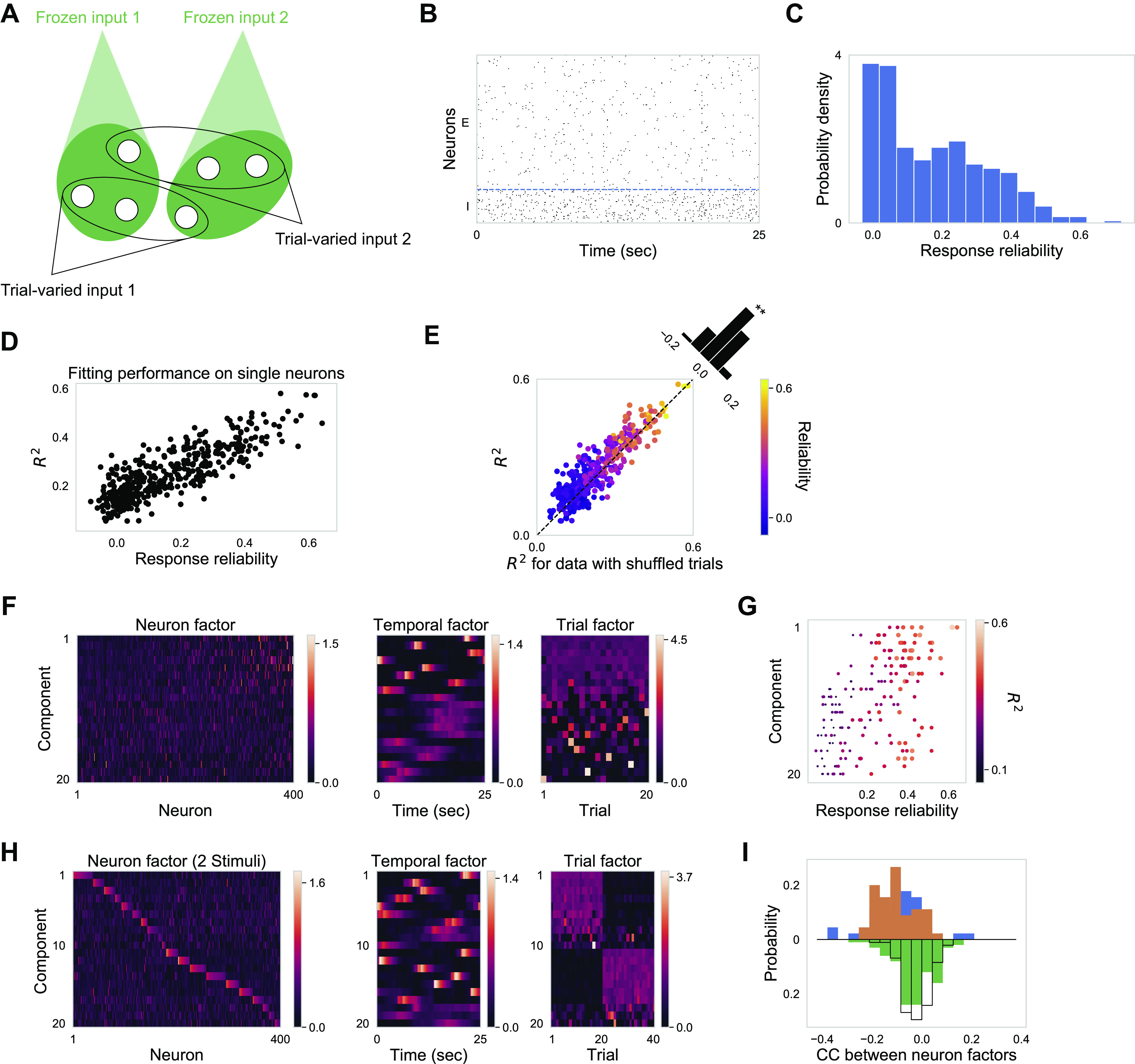
A balanced network model with random connectivity and clustered external inputs reproduces key features of observed cortical activity. A: illustration for the input structure to the model network. We simulated a balanced network with uniform random connectivity. There are two types of external inputs: frozen input pulse trains and trial-varied input pulse trains. Both inputs have a clustered input structure but with different neuron partitions. Model network consists of 1,600 excitatory neurons and 400 inhibitory neurons. Twenty-five seconds × 20 trials are simulated. B: raster plot of 500 randomly subsampled neurons during one trial. Blue dashed line separates inhibitory neurons from excitatory neurons. C: response reliability histogram for subsampled excitatory neurons. Response reliability is calculated based on simulated ∆F/F traces. D: fitting performance R² (20 TCA components) plotted against response reliability for subsampled excitatory neurons. E: fitting performance R² for original data plotted against R² for data with shuffled trials for subsampled excitatory neurons (Mann–Whitney rank test, P < 0.005). Color indicates response reliability. F: 20 TCA components. Components are ordered by CV of trial factors. In neuron factor, neurons are ordered by their response reliability. G: reliability of 10 neurons with the largest neuron factor values for different components. Components are in the same order as in F. H: 20 TCA components for concatenated neural responses to two stimuli. Neuron factors are plotted with neurons ordered by their dominant components (see methods). I: distribution of CC between neuron factors. Color code is the same as Fig. 5G: orange is for CC between neuron factors during stimulus one; blue is for CC between neuron factors during stimulus two; green is for CC between neuron factors across stimuli; black is for CC between random vectors with the same dimension as neuron factors, representing the chance level. Both CC during stimulus 1 and CC during stimulus 2 are significantly negative (one-sample t test, P < 0.001), and CC across stimuli is centered around zero (one-sample t test, P = 0.23). CC, correlation coefficient; CV, coefficient of variation TCA, tensor component analysis.

With a choice of appropriate set of parameters, key features of the observed cortical activity were reproduced by the model network (Fig. 6). Even though model neurons received highly correlated external inputs, they operated in an asynchronous state (Fig. 6B) due to balanced excitatory and inhibitory recurrent inputs (Renart et al. 2010). In addition, with lognormal distributed synaptic weights of external inputs (Supplemental Fig. S4B), the model exhibited a skewed distribution of response reliability (Fig. 6C). Furthermore, consistent with experimental results, simulated activities of model neurons were well fitted by TCA (Fig. 6D) and they covaried more than expected by chance (Fig. 6E). Moreover, both consistent and inconsistent components recruited neurons with a range of reliabilities (Fig. 6, F and G). Importantly, when the model network was presented with two different stimuli (see methods), intercomponent CCs within stimuli were predominantly negative, whereas intercomponent CCs across stimuli centered around zero (Fig. 6, H and I).

By reproducing the observed cortical dynamics, the model revealed several essential insights. First, the clustered structure in external inputs, instead of the clustered structure in recurrent connections (Fig. 7, A–C), is more likely to support the observed coactivation pattern in neuronal responses. Clustered recurrent connections would lead to spontaneous slow dynamics during which neurons within the cluster transiently increased or decreased their firing rate (Litwin-Kumar and Doiron 2012). This spontaneous slow dynamics results in multiple inconsistent components with different temporal factors but the same neuron factors (Fig. 7C), which is contradictory to the experimental results. In contrast, TCA components of the model with clustered external inputs and random connectivity qualitatively resembled TCA components from experimental data (Fig. 6). Second, to impose coactivation patterns on neurons with a range of reliabilities, each neuron needs to receive two kinds of inputs: (1) frozen input pulse train imitating a stimulus-driven variable and (2) trial-varied input pulse train imitating a stimulus-independent variable. If each neuron received either the frozen or the trial-varied input pulse train (Fig. 7D), then neurons’ coactivation pattern would be determined by neuron’s reliability (Fig. 7, E and F; Fig. 1B, the constrained case). Third, it is important to have balanced recurrent connections to keep neural activity in the asynchronous regime. Without the recurrent connections, neural activity would become synchronous to the external inputs. Moreover, the chaotic nature of the balanced network (van Vreeswijk and Sompolinsky 1998) contributed to model high trial-to-trial variability in neural activity.

Fig. 7.

Alternative model networks failed to reproduce observed key features of neuronal coactivation patterns. A–C: the model network with clustered recurrent connections failed to reproduce key features of neuron factors. A: connectivity weights between neurons in the model network with clustered excitatory connections. The excitatory population was partitioned into clusters of 100 neurons each. The connection probability within the cluster was 1.7 times as much as the connection probability between clusters. The connection strength between excitatory neurons from the same cluster was 1.9 times as much as the connection strength between excitatory neurons from different clusters. On average, each neuron received 200 excitatory recurrent inputs. B: raster plot of 500 randomly subsampled neurons during one trial. Blue dashed line separates inhibitory neurons from excitatory neurons. Note that neurons within the same cluster fire together irregularly. C: 20 TCA components for neural responses ordered by consistency of their trial factors. Here, some inconsistent components have highly correlated neuron factors, due to the spontaneous slow dynamics (see B) in the model network with clustered excitatory connections. D–F: the model network with a unique input structure failed to reproduce coactivation patterns independent of reliability. D: illustration for input structure to model network. Frozen input pulse trains and trial-varied input pulse trains project to different groups of neurons. E: reliability of 10 neurons with the largest neuron factor values for different components. Components are in the same order as in C. F: 20 TCA components. Components are ordered by CV of trial factors. In neuron factor, neurons are ordered by their response reliability. CV, coefficient of variation TCA, tensor component analysis.

In conclusion, this analysis of recurrent balanced neural network models revealed that both the stimulus specificity and the mixed encoding of qualitatively different variables can arise from clustered external inputs.

DISCUSSION

Neural variability is widely studied as a single-neuron feature (Faisal et al. 2008; Mainen and Sejnowski 1995) and a population-wide feature (Cohen and Kohn 2011; Doiron et al. 2016). Here, we related single-neuron variability to population-wide variability by asking how neurons with different levels of reliability encode unobserved variables. Our work demonstrated that neurons spanning a range of reliabilities are coactive and encode a mixture of stimulus-driven and stimulus-independent unobserved variables. We found that a neuron’s response reliability and the neuronal coactivation patterns substantially reorganized for different external visual inputs. Furthermore, our model suggested clustered external inputs underpin the observed coactivation pattern of neurons. More broadly, this study has made the following contributions to our understanding of connectivity-mediated variability in the visual cortex.

First, we found that neural variability is well captured by additive and multiplicative modulation shared across neuron ensembles, as shown by the applicability of the linear TCA analysis (Fig. 2, A and B). Neural variability can be modeled as an additive modulation (Schölvinck et al. 2015) by summing the trial-averaged evoked response and some stochastic activity such as spontaneous activity (Arieli et al. 1996). Alternatively, neural variability can be modeled as a multiplicative modulation (Ecker et al. 2014; Goris et al. 2014) by multiplying the trial-averaged evoked response with a gain factor. Both additive and multiplicative modulations are necessary to reproduce neural variability observed in experimental data (Arandia-Romero et al. 2016; Lin et al. 2015). Here, we modeled trial-to-trial variability as a sum of gain-changed temporal factors, where the gain is governed by the corresponding neuron factor and trial factor. Note that the temporal factors represent the shared neural activity across neurons and trials, which might serve as a better neural basis than the trial-averaged evoked responses (Williams et al. 2018). However, as TCA is built to capture shared modulation across dimensions, it is unlikely to capture independent multiplicative or additive modulations. For example, the gain modulation of the neuron with low reliability shown in Fig. 3C was not captured by TCA, given a limited number of components.

Second, we found that individual neuron’s response reliability imposes only a weak constraint on its encoding capabilities. One explanation given for the presence of neurons exhibiting weak responses to sensory stimuli is that even poorly driven neurons may contribute to sensory coding (Leavitt et al. 2017; Safaai et al. 2013). Indeed, we show that neurons with low reliability often make strong contributions to consistent stimulus-driven factors, despite the fact that the responses of individual neurons can be highly variable across trials (Fig. 3). In contrast, researchers have proposed that variable activity across trials is due to coding of nonsensory information, such as motor or behavioral variables (Niell and Stryker 2010; Vinck et al. 2015). A recent article using shared variance component analysis identified stimulus-independent latent factors that were linked to facial movements and drove visual cortical neurons independently of sensory input (Stringer et al. 2019b). Our results are also in agreement with this finding, as we show that neurons from a range of reliabilities contribute to stimulus-independent latent factors (Fig. 3). Taken together, these results show that the encoding of distinct variables is not mutually exclusive and that both phenomena are evident in visual cortical networks.

Third, our experiment and model results support the possibility that clustered external inputs underpin the neuronal coactivation pattern. Alternatively, coactive neuronal ensembles could result from structured recurrent connectivity, based on the fact that the connectivity probability between coactive neurons is higher than neurons with decorrelated evoked responses (Ko et al. 2011). Additional evidence in support of this alternative mechanism is the similarity between coactive neuronal ensembles during spontaneous and stimulus-modulated activity (MacLean et al. 2005; Miller et al. 2014). However, the evidence might not be sufficient: A neural network with random connectivity can also generate similar neuronal coactivation patterns during spontaneous and evoked activity (Okun et al. 2012). Moreover, consistent with previous work (Hofer et al. 2011), we found that neuronal coactivation pattern is highly dependent on stimulus (Fig. 5), which demonstrated that external inputs, instead of recurrent connection, may be the dominant factor in the formation of neuronal ensembles. The mechanism underlying these coactivation patterns is still unclear. Searching for further evidence for our proposed mechanism might require analyses on simultaneous recordings from external inputs and cortical neurons (Sun et al. 2016).

Fourth, the coactivation pattern of neurons with diverse reliability provides insights on the connectivity of external inputs to visual cortex. Neuroanatomy data showed that V1 in mice is highly interconnected with other regions of neocortex (Froudarakis et al. 2019). For instance, V1 receives inputs carrying sensorimotor information (Petreanu et al. 2012). However, the structure of inputs at the neuronal population level remains elusive. In Fig. 1, we described a spectrum of how neurons encode stimulus-driven and stimulus-independent variables. Based on model investigations (Figs. 6 and 7, D–F), the two extremes of the spectrum correspond to different external input structures. Our experimental and model results suggested that a neuron’s reliability imposes only a weak constraint on its encoding capability, indicating that neurons receive both frozen and trial-varied inputs. This input paradigm has a potential functional advantage such that fewer neurons are required to encode the same number of variables, compared with distinct external inputs projecting to separate groups of neurons. Furthermore, different variables are encoded by largely nonoverlapped groups of neurons within a stimulus set (Fig. 5). This nonoverlapping encoding strategy indicates that each input tends to innervate different groups of neurons. Such a mutually exclusive representation may enable simple linear readout for downstream neurons. This trade-off between efficient coding and high readout efficiency informed the choice of the input structure in our model. However, the chosen input structure in our model may not be the only possible solution to reproduce the key features of neuronal coactivation patterns. Another limitation of our model is that we assumed random connectivity between model neurons, which is not true for cortical neurons. Models with spatial dependence in connectivity resembling cortical networks (Huang et al. 2019) are good candidates to be investigated in the future.

An important next step is to identify what stimulus-driven and stimulus-independent variables are encoded by neural responses. Earlier work suggests two possible ways to identify the stimulus-independent variables. First, we can look for behavioral or internal variables that have the highest correlation with the trial factors of inconsistent components (Hirokawa et al. 2019; Stringer et al. 2019b). Second, we can use photostimulation to activate the neuronal ensemble corresponding to the stimulus-independent component and observe the changes of behavioral variables (Carrillo-Reid et al. 2019). However, it is much less straightforward to identify the stimulus-driven variables or visual features in this case. One promising idea is using a generative closed-loop system to evolve synthetic images to maximize the corresponding neuronal ensemble’s coactivation (Bashivan et al. 2019; Ponce et al. 2019). Such evolved images might provide insight on the visual features encoded by the particular neuron ensemble.

GRANTS

This work was supported by the following grants: Whitehall Foundation #20121221 (to R.Wessel), NSF CRCNS #1308159 (to R.Wessel), NIH R00 MH104259 (to M. J. Goard), Whitehall Foundation #20181228 (to M. J. Goard), and NSF NeuroNex #1707287 (to M. J. Goard).

DISCLOSURES

No conflicts of interest, financial or otherwise, are declared by the authors.

AUTHOR CONTRIBUTIONS

J.X., M.J.G., and R.W. conceived and designed research; T.D.M. performed experiments; J.X. analyzed data; J.X., T.D.M., M.J.G., and R.W. interpreted results of experiments; J.X. prepared figures; J.X. drafted manuscript; J.X., T.D.M., M.J.G., and R.W. edited and revised manuscript; J.X., T.D.M., M.J.G., and R.W. approved final version of manuscript.

REFERENCES

- Allen WE, Chen MZ, Pichamoorthy N, Tien RH, Pachitariu M, Luo L, Deisseroth K. Thirst regulates motivated behavior through modulation of brainwide neural population dynamics. Science 364: 253, 2019. doi: 10.1126/science.aav3932. [DOI] [PMC free article] [PubMed] [Google Scholar]
- Arandia-Romero I, Tanabe S, Drugowitsch J, Kohn A, Moreno-Bote R. Multiplicative and additive modulation of neuronal tuning with population activity affects encoded information. Neuron 89: 1305–1316, 2016. doi: 10.1016/j.neuron.2016.01.044. [DOI] [PMC free article] [PubMed] [Google Scholar]
- Arieli A, Sterkin A, Grinvald A, Aertsen A. Dynamics of ongoing activity: explanation of the large variability in evoked cortical responses. Science 273: 1868–1871, 1996. doi: 10.1126/science.273.5283.1868. [DOI] [PubMed] [Google Scholar]
- Bashivan P, Kar K, DiCarlo JJ. Neural population control via deep image synthesis. Science 364: eaav9436, 2019. doi: 10.1126/science.aav9436. [DOI] [PubMed] [Google Scholar]
- Brainard DH. The Psychophysics Toolbox. Spat Vis 10: 433–436, 1997. doi: 10.1163/156856897X00357. [DOI] [PubMed] [Google Scholar]
- Buzsáki G. Neural syntax: cell assemblies, synapsembles, and readers. Neuron 68: 362–385, 2010. doi: 10.1016/j.neuron.2010.09.023. [DOI] [PMC free article] [PubMed] [Google Scholar]
- Carrillo-Reid L, Han S, Yang W, Akrouh A, Yuste R. Controlling visually guided behavior by holographic recalling of cortical ensembles. Cell 178: 447–457.e5, 2019. doi: 10.1016/j.cell.2019.05.045. [DOI] [PMC free article] [PubMed] [Google Scholar]
- Cohen MR, Kohn A. Measuring and interpreting neuronal correlations. Nat Neurosci 14: 811–819, 2011. doi: 10.1038/nn.2842. [DOI] [PMC free article] [PubMed] [Google Scholar]
- Dipoppa M, Ranson A, Krumin M, Pachitariu M, Carandini M, Harris KD. Vision and locomotion shape the interactions between neuron types in mouse visual cortex. Neuron 98: 602–615.e8, 2018. doi: 10.1016/j.neuron.2018.03.037. [DOI] [PMC free article] [PubMed] [Google Scholar]
- Doiron B, Litwin-Kumar A, Rosenbaum R, Ocker GK, Josić K. The mechanics of state-dependent neural correlations. Nat Neurosci 19: 383–393, 2016. doi: 10.1038/nn.4242. [DOI] [PMC free article] [PubMed] [Google Scholar]
- Douglas RJ, Koch C, Mahowald M, Martin KA, Suarez HH. Recurrent excitation in neocortical circuits. Science 269: 981–985, 1995. doi: 10.1126/science.7638624. [DOI] [PubMed] [Google Scholar]
- Ecker AS, Berens P, Cotton RJ, Subramaniyan M, Denfield GH, Cadwell CR, Smirnakis SM, Bethge M, Tolias AS. State dependence of noise correlations in macaque primary visual cortex. Neuron 82: 235–248, 2014. doi: 10.1016/j.neuron.2014.02.006. [DOI] [PMC free article] [PubMed] [Google Scholar]
- Faisal AA, Selen LP, Wolpert DM. Noise in the nervous system. Nat Rev Neurosci 9: 292–303, 2008. doi: 10.1038/nrn2258. [DOI] [PMC free article] [PubMed] [Google Scholar]
- Froudarakis E, Fahey PG, Reimer J, Smirnakis SM, Tehovnik EJ, Tolias AS. The visual cortex in context. Annu Rev Vis Sci 5: 317–339, 2019. doi: 10.1146/annurev-vision-091517-034407. [DOI] [PMC free article] [PubMed] [Google Scholar]
- Goard M, Dan Y. Basal forebrain activation enhances cortical coding of natural scenes. Nat Neurosci 12: 1444–1449, 2009. doi: 10.1038/nn.2402. [DOI] [PMC free article] [PubMed] [Google Scholar]
- Goris RLT, Movshon JA, Simoncelli EP. Partitioning neuronal variability. Nat Neurosci 17: 858–865, 2014. doi: 10.1038/nn.3711. [DOI] [PMC free article] [PubMed] [Google Scholar]
- Hirokawa J, Vaughan A, Masset P, Ott T, Kepecs A. Frontal cortex neuron types categorically encode single decision variables. Nature 576: 446–451, 2019. doi: 10.1038/s41586-019-1816-9. [DOI] [PMC free article] [PubMed] [Google Scholar]
- Hofer SB, Ko H, Pichler B, Vogelstein J, Ros H, Zeng H, Lein E, Lesica NA, Mrsic-Flogel TD. Differential connectivity and response dynamics of excitatory and inhibitory neurons in visual cortex. Nat Neurosci 14: 1045–1052, 2011. doi: 10.1038/nn.2876. [DOI] [PMC free article] [PubMed] [Google Scholar]
- Huang C, Ruff DA, Pyle R, Rosenbaum R, Cohen MR, Doiron B. Circuit models of low-dimensional shared variability in cortical networks. Neuron 101: 337–348.e4, 2019. doi: 10.1016/j.neuron.2018.11.034. [DOI] [PMC free article] [PubMed] [Google Scholar]
- Keemink SW, Machens CK. Decoding and encoding (de)mixed population responses. Curr Opin Neurobiol 58: 112–121, 2019. doi: 10.1016/j.conb.2019.09.004. [DOI] [PubMed] [Google Scholar]
- Ko H, Hofer SB, Pichler B, Buchanan KA, Sjöström PJ, Mrsic-Flogel TD. Functional specificity of local synaptic connections in neocortical networks. Nature 473: 87–91, 2011. doi: 10.1038/nature09880. [DOI] [PMC free article] [PubMed] [Google Scholar]
- Kobak D, Brendel W, Constantinidis C, Feierstein CE, Kepecs A, Mainen ZF, Qi X-L, Romo R, Uchida N, Machens CK. Demixed principal component analysis of neural population data. eLife 5: e10989, 2016. doi: 10.7554/eLife.10989. [DOI] [PMC free article] [PubMed] [Google Scholar]
- Kruskal JB. Three-way arrays: rank and uniqueness of trilinear decompositions, with application to arithmetic complexity and statistics. Linear Algebra Appl 18: 95–138, 1977. doi: 10.1016/0024-3795(77)90069-6. [DOI] [Google Scholar]
- Leavitt ML, Pieper F, Sachs AJ, Martinez-Trujillo JC. Correlated variability modifies working memory fidelity in primate prefrontal neuronal ensembles. Proc Natl Acad Sci USA 114: E2494–E2503, 2017. doi: 10.1073/pnas.1619949114. [DOI] [PMC free article] [PubMed] [Google Scholar]
- Lin I-C, Okun M, Carandini M, Harris KD. The nature of shared cortical variability. Neuron 87: 644–656, 2015. doi: 10.1016/j.neuron.2015.06.035. [DOI] [PMC free article] [PubMed] [Google Scholar]
- Litwin-Kumar A, Doiron B. Slow dynamics and high variability in balanced cortical networks with clustered connections. Nat Neurosci 15: 1498–1505, 2012. doi: 10.1038/nn.3220. [DOI] [PMC free article] [PubMed] [Google Scholar]
- MacLean JN, Watson BO, Aaron GB, Yuste R. Internal dynamics determine the cortical response to thalamic stimulation. Neuron 48: 811–823, 2005. doi: 10.1016/j.neuron.2005.09.035. [DOI] [PubMed] [Google Scholar]
- Madisen L, Garner AR, Shimaoka D, Chuong AS, Klapoetke NC, Li L, van der Bourg A, Niino Y, Egolf L, Monetti C, Gu H, Mills M, Cheng A, Tasic B, Nguyen TN, Sunkin SM, Benucci A, Nagy A, Miyawaki A, Helmchen F, Empson RM, Knöpfel T, Boyden ES, Reid RC, Carandini M, Zeng H. Transgenic mice for intersectional targeting of neural sensors and effectors with high specificity and performance. Neuron 85: 942–958, 2015. doi: 10.1016/j.neuron.2015.02.022. [DOI] [PMC free article] [PubMed] [Google Scholar]
- Mainen ZF, Sejnowski TJ. Reliability of spike timing in neocortical neurons. Science 268: 1503–1506, 1995. doi: 10.1126/science.7770778. [DOI] [PubMed] [Google Scholar]
- Mante V, Sussillo D, Shenoy KV, Newsome WT. Context-dependent computation by recurrent dynamics in prefrontal cortex. Nature 503: 78–84, 2013. doi: 10.1038/nature12742. [DOI] [PMC free article] [PubMed] [Google Scholar]
- McGinley MJ, David SV, McCormick DA. Cortical membrane potential signature of optimal states for sensory signal detection. Neuron 87: 179–192, 2015. doi: 10.1016/j.neuron.2015.05.038. [DOI] [PMC free article] [PubMed] [Google Scholar]
- Miller J-EK, Ayzenshtat I, Carrillo-Reid L, Yuste R. Visual stimuli recruit intrinsically generated cortical ensembles. Proc Natl Acad Sci USA 111: E4053–E4061, 2014. doi: 10.1073/pnas.1406077111. [DOI] [PMC free article] [PubMed] [Google Scholar]
- Niell CM, Stryker MP. Modulation of visual responses by behavioral state in mouse visual cortex. Neuron 65: 472–479, 2010. doi: 10.1016/j.neuron.2010.01.033. [DOI] [PMC free article] [PubMed] [Google Scholar]
- Okun M, Yger P, Marguet SL, Gerard-Mercier F, Benucci A, Katzner S, Busse L, Carandini M, Harris KD. Population rate dynamics and multineuron firing patterns in sensory cortex. J Neurosci 32: 17108–17119, 2012. doi: 10.1523/JNEUROSCI.1831-12.2012. [DOI] [PMC free article] [PubMed] [Google Scholar]
- Olshausen BA, Field DJ. What is the other 85 percent of V1 doing? In: 23 Problems in Systems Neuroscience, edited by van Hemmen JL, Sejnowski TJ. Oxford, UK: Oxford University Press, 2006, p. 182–212. [Google Scholar]
- Petreanu L, Gutnisky DA, Huber D, Xu N-L, O’Connor DH, Tian L, Looger L, Svoboda K. Activity in motor-sensory projections reveals distributed coding in somatosensation. Nature 489: 299–303, 2012. doi: 10.1038/nature11321. [DOI] [PMC free article] [PubMed] [Google Scholar]
- Ponce CR, Xiao W, Schade PF, Hartmann TS, Kreiman G, Livingstone MS. Evolving images for visual neurons using a deep generative network reveals coding principles and neuronal preferences. Cell 177: 999–1009.e10, 2019. doi: 10.1016/j.cell.2019.04.005. [DOI] [PMC free article] [PubMed] [Google Scholar]
- Renart A, de la Rocha J, Bartho P, Hollender L, Parga N, Reyes A, Harris KD. The asynchronous state in cortical circuits. Science 327: 587–590, 2010. doi: 10.1126/science.1179850. [DOI] [PMC free article] [PubMed] [Google Scholar]
- Rikhye RV, Sur M. Spatial correlations in natural scenes modulate response reliability in mouse visual cortex. J Neurosci 35: 14661–14680, 2015. doi: 10.1523/JNEUROSCI.1660-15.2015. [DOI] [PMC free article] [PubMed] [Google Scholar]
- Safaai H, von Heimendahl M, Sorando JM, Diamond ME, Maravall M. Coordinated population activity underlying texture discrimination in rat barrel cortex. J Neurosci 33: 5843–5855, 2013. doi: 10.1523/JNEUROSCI.3486-12.2013. [DOI] [PMC free article] [PubMed] [Google Scholar]
- Saxena S, Cunningham JP. Towards the neural population doctrine. Curr Opin Neurobiol 55: 103–111, 2019. doi: 10.1016/j.conb.2019.02.002. [DOI] [PubMed] [Google Scholar]
- Schölvinck ML, Saleem AB, Benucci A, Harris KD, Carandini M. Cortical state determines global variability and correlations in visual cortex. J Neurosci 35: 170–178, 2015. doi: 10.1523/JNEUROSCI.4994-13.2015. [DOI] [PMC free article] [PubMed] [Google Scholar]
- Softky WR, Koch C. The highly irregular firing of cortical cells is inconsistent with temporal integration of random EPSPs. J Neurosci 13: 334–350, 1993. doi: 10.1523/JNEUROSCI.13-01-00334.1993. [DOI] [PMC free article] [PubMed] [Google Scholar]
- Stringer C, Pachitariu M, Steinmetz N, Carandini M, Harris KD. High-dimensional geometry of population responses in visual cortex. Nature 571: 361–365, 2019a. doi: 10.1038/s41586-019-1346-5. [DOI] [PMC free article] [PubMed] [Google Scholar]
- Stringer C, Pachitariu M, Steinmetz N, Reddy CB, Carandini M, Harris KD. Spontaneous behaviors drive multidimensional, brainwide activity. Science 364: eaav7893, 2019b. doi: 10.1126/science.aav7893. [DOI] [PMC free article] [PubMed] [Google Scholar]
- Sun W, Tan Z, Mensh BD, Ji N. Thalamus provides layer 4 of primary visual cortex with orientation- and direction-tuned inputs. Nat Neurosci 19: 308–315, 2016. doi: 10.1038/nn.4196. [DOI] [PMC free article] [PubMed] [Google Scholar]
- van Vreeswijk C, Sompolinsky H. Chaos in neuronal networks with balanced excitatory and inhibitory activity. Science 274: 1724–1726, 1996. doi: 10.1126/science.274.5293.1724. [DOI] [PubMed] [Google Scholar]
- van Vreeswijk C, Sompolinsky H. Chaotic balanced state in a model of cortical circuits. Neural Comput 10: 1321–1371, 1998. doi: 10.1162/089976698300017214. [DOI] [PubMed] [Google Scholar]
- Vinck M, Batista-Brito R, Knoblich U, Cardin JA. Arousal and locomotion make distinct contributions to cortical activity patterns and visual encoding. Neuron 86: 740–754, 2015. doi: 10.1016/j.neuron.2015.03.028. [DOI] [PMC free article] [PubMed] [Google Scholar]
- Williams AH, Kim TH, Wang F, Vyas S, Ryu SI, Shenoy KV, Schnitzer M, Kolda TG, Ganguli S. Unsupervised discovery of demixed, low-dimensional neural dynamics across multiple timescales through tensor component analysis. Neuron 98: 1099–1115.e8, 2018. doi: 10.1016/j.neuron.2018.05.015. [DOI] [PMC free article] [PubMed] [Google Scholar]
- Yuste R. From the neuron doctrine to neural networks. Nat Rev Neurosci 16: 487–497, 2015. doi: 10.1038/nrn3962. [DOI] [PubMed] [Google Scholar]