Simplifying Transforms for General Elastic Metrics on the Space of Plane Curves

Abstract

In the shape analysis approach to computer vision problems, one treats shapes as points in an infinite-dimensional Riemannian manifold, thereby facilitating algorithms for statistical calculations such as geodesic distance between shapes and averaging of a collection of shapes. The performance of these algorithms depends heavily on the choice of the Riemannian metric. In the setting of plane curve shapes, attention has largely been focused on a two-parameter family of first order Sobolev metrics, referred to as elastic metrics. They are particularly useful due to the existence of simplifying coordinate transformations for particular parameter values, such as the well-known square-root velocity transform. In this paper, we extend the transformations appearing in the existing literature to a family of isometries, which take any elastic metric to the flat L² metric. We also extend the transforms to treat piecewise linear curves and demonstrate the existence of optimal matchings over the diffeomorphism group in this setting. We conclude the paper with multiple examples of shape geodesics for open and closed curves. We also show the benefits of our approach in a simple classification experiment.

1. Introduction.

Shape is a fundamental physical property of objects and plays an important role in various imaging tasks, including identification and tracking. As a result, statistical analysis of shape plays a crucial role in many image-rich application domains such as computer vision, medical imaging, biology, bioinformatics, geology, and biometrics. In statistical shape analysis, shape is viewed as a random object, and one is concerned with developing methods to perform common statistical tasks, including registration, comparison, averaging, summarization of variability, hypothesis testing, regression, and other inferential procedures. Any statistical shape analysis approach requires an appropriate shape representation and an associated metric that enables quantification of shape differences. Evidently, the quality of statistical analyses of shape data is heavily dependent on these choices.

There is a rich literature on statistical analysis of shape, with the most prominent shape representation being landmark-based. Landmarks constitute a finite collection of points that are chosen either by the application expert (anatomical landmarks) or according to some mathematical rule such as high absolute curvature (mathematical landmarks). Once the points are selected, the remaining information regarding the object’s outline is discarded. Under this representation, Kendall [25] defined shape as a property of an object that is invariant to its rigid motions and global scaling; this approach is commonly referred to as similarity shape analysis. Since then, there has been continuous development of statistical tools to analyze similarity shapes represented by landmarks; see [17, 43] for a comprehensive set of methods. These approaches combine ideas from differential geometry, algebra, and multivariate statistics to establish rigorous estimation and inferential procedures on the landmark shape space. The main benefit of these approaches is that the resulting shape space is finite-dimensional, making statistical analysis “easier.” However, the obvious drawback is that the finite collection of landmarks used to represent shapes of interest results in significant loss of information.

Recently, there has been more emphasis on using a function-based representation of shape, i.e., objects are represented via their boundaries as parameterized curves. Thus, in this case, one must account for possible parameterization variability in addition to rigid motion and global scaling. One set of methods removes this variability by normalizing all parameterizations to arclength [26, 56]. However, such an approach is suboptimal in many real scientific problems due to a lack of appropriate registration. A better approach is to remove such variability in a pairwise manner using an appropriate metric. This is the idea behind elastic shape analysis, where a family of elastic metrics is used for joint registration and comparison. The resulting shape spaces are more complicated than their landmark counterparts, but the benefits of such approaches are clear: (1) there is no need to select landmarks, which can be a tedious and expensive process; (2) the curve representation is able to encode all relevant shape information; and (3) the elastic metric quantifies intuitive shape deformations. Elastic shape analysis is the focus of the current paper, and we provide a formal mathematical setup for this approach in the following section.

1.1. Elastic shape analysis.

A fundamental ingredient in a theory of shape similarity for plane curves is a distance metric on the space of curves $\mathcal{S}$ which is invariant under rigid transformations of the curves. For a pair of plane curves C₁ and C₂, we therefore wish to assign a distance d(C₁, C₂) such that d(ξ₁ ⋆ C₁, ξ₂ ⋆ C₂) = d(C₁, C₂) for any elements ξ_j of the Euclidean isometry group ${ℝ}^2⋉\text{SO}(2)$, acting in the natural way.

Under the elastic shape analysis paradigm, the distance function described above arises from a Riemannian metric. This extra structure has obvious benefits over treating $\mathcal{S}$ only as a metric space; for example, it allows the potential to compute geodesic curve deformations and to locally linearize via the logarithm map in order to do statistics in a tangent space. The metric on the space of (unparameterized) curves $\mathcal{S}$ is obtained by treating it as a quotient space, described as follows. Let $I\subset ℝ$ denote some fixed interval, $\text{Imm}\left(I,{ℝ}^2\right)\subset C^{\infty }\left(I,{ℝ}^2\right)$ the open submanifold of smooth immersions, and Diff⁺(I) the Lie group of orientation-preserving diffeomorphisms of I. This group acts on $\text{Imm}\left(I,{ℝ}^2\right)$ by reparameterizations. We then represent the space of curves as $\mathcal{S}\approx \text{Imm}\left(I,{ℝ}^2\right)/{\text{Diff}}^{+}(I)$; in other words, the space of unparameterized curves is realized as the space of parameterized curves identified up to reparameterizations. A choice g of Diff⁺(I)-invariant Riemannian metric on the relatively simple space $\text{Imm}\left(I,{ℝ}^2\right)$ descends to a well-defined metric on $\mathcal{S}$. If the Riemannian metric is also invariant under Euclidean similarities, then the geodesic distance with respect to this metric induces our desired distance function d via the formula

$$d\left(C_1,C_2\right)=\underset{{\sigma }_1,{\sigma }_2\in {\text{ Diff }}^{+}(I)\times \left({ℝ}^2\times SO(2)\right)}{\text{inf}}{\text{dist}}_g\left({\sigma }_1\star c_1,{\sigma }_2\star c_2\right).$$

In this formula, the c_j are arbitrary choices of parameterizations of C_j, dist_g denotes geodesic distance in $\text{Imm}\left(I,{ℝ}^2\right)$ with respect to g, and ⋆ denotes the action of the group ${\text{Diff }}^{+}(I)\times \left({ℝ}^2⋉\text{SO}(2)\right)$ of shape-preserving transformations on $\text{Imm}\left(I,{ℝ}^2\right)$, defined as follows. A triple $\sigma =(\gamma ,v,A)\in {\text{Diff}}^{+}(I)\times \left({ℝ}^2⋉\text{SO}(2)\right)$ acts on a curve c by reparameterizing by γ, rotating c about c(0) by A, and translating the image of c by v.

The simplest choice of Riemannian metric is the reparameterization-invariant L² metric defined for $c\in \text{Imm}\left(I,{ℝ}^2\right)$ and $h,k\in T_c\text{Imm}\left(I,{ℝ}^2\right)\approx C^{\infty }\left(I,{ℝ}^2\right)$ by the formula

$${\widehat{g}}_c^{L^2}(h,k)={\int }_I\langle h,k\rangle \text{ d}s.$$

The notation $\widehat{g}$ is used to distinguish this metric from the standard (non-reparameterization-invariant) L² metric which will appear later in the paper. The nonlinearity of this metric lies in the measure with respect to arclength ds = |c′(t)| dt, which provides the desired Diff⁺(I)-invariance. It is a surprising fact that geodesic distance on the shape space vanishes with respect to ${\widehat{g}}^{L^2}$ [34], and one must therefore consider more complicated metrics on the space of immersions. Examples in the literature of such metrics include almost-local (weighted L²) metrics [7, 8, 35] and higher order Sobolev-type metrics [6, 15, 35, 46]. An element of the latter class of metrics is a natural generalization of the reparameterization-invariant L² metric, defined by

$$g_c^{\overrightarrow{d}}(h,k)={\int }_I{a}_0^2\langle h,k\rangle +a_1^2\langle D_{s}h,D_{s}k\rangle +\cdots +a_n^2\langle D_s^{n}h,D_s^{n}k\rangle \text{ d}s,$$

where $\overrightarrow{a}=\left(a_0,a_1,\dots ,a_n\right)$ is a vector of weights on the terms, and we use $D_s=\frac{1}{c^{\prime }(t)}\frac{d}{dt}$ for derivative with respect to arclength. The higher order Sobolev metrics no longer suffer the vanishing geodesic phenomenon and are, in fact, geodesically complete when a₀, a_n > 0 for n ⩾ 2 [12].

A particularly well-studied subfamily of first order (i.e., n = 1 in the above notation) Sobolev metrics are the elastic metrics introduced in [37]. These form a two-parameter family of metrics g^a,b defined by setting a₀ = 0 and further decomposing the first order term into tangential and normal components. That is, for $c\in \text{Imm}\left(I,{ℝ}^2\right)$, let (T, N) denote the standard moving frame consisting of the unit tangent and unit normal to c, respectively. For a, b ≠ 0 and $h,k\in T_c\text{Imm}\left(I,{ℝ}^2\right)$, we define

$$g_c^{a,b}(h,k)={\int }_I{a}^2\langle D_{s}h,N\rangle \langle D_{s}k,N\rangle +b^2\langle D_{s}h,T\rangle \langle D_{s}k,T\rangle \text{ d}s.$$ (1.1)

This metric is invariant under reparameterizations and rigid motions, and so descends to a well-defined metric on the shape space $\mathcal{S}$. While these metrics do not enjoy the geodesic completeness of their higher order counterparts, we will see below that they have a number of useful theoretical properties and, in particular, that geodesic distance is nonvanishing. This paper will focus exclusively on this family of elastic metrics.

1.2. Previous work on elastic metrics.

In order to compute the distance between curves in $\mathcal{S}$, our procedure requires the computation of geodesic distance with respect to the chosen metric. Early approaches to this task accomplished this by explicitly solving the associated variational problems [47, 48, 53]. Focusing on the elastic metric g^1,1/2, a common technique is to apply the square-root velocity function (SRVF) transform, given by

$$\text{Imm}\left(I,{ℝ}^2\right)\to C^{\infty }\left(I,{ℝ}^2\right),$$

$$c\mapsto \frac{c^{\prime }}{{\left|c^{\prime }\right|}^{1/2}}.$$

The theoretical power of the SRVF is the remarkable fact that the pullback of the standard L² metric on the target space is the elastic metric g^1,1/2 [24], whence geodesics with respect to g^1,1/2 in $\text{Imm}\left(I,{ℝ}^2\right)$ can be computed explicitly by pushing forward to the flat target space, computing geodesics there, then pulling the result back. Due to this convenient property, the SRVF transform has been studied extensively from a theoretical perspective [11, 31, 44, 49] and has seen a wide variety of applications, including classification of plant leaf shapes [30], statistical analysis of protein structures [45], and biomedical imaging of anatomical features in the brain [2]. A similarly simple transform is introduced in [55], where a plane curve c is taken to the curve $\sqrt{c^{\prime }}$, with the square root taken pointwise by considering c′ to be a path in the complex plane; in this case, the map pulls back the L² metric to g^1/2,1/2. A more complicated family of transforms R_a,b is defined in [5] for 2b ⩾ a > 0, and it is shown that the pullback by R_a,b of the L² metric on its target is g^a,b. A different framework for understanding general elastic metrics, with a more explicit focus on the various Lie group actions, is provided in [54]. There has also been substantial effort put toward numerical computations for geodesics in spaces of curves with respect to these metrics (and more general Sobolev-type metrics); see, e.g., [4, 3].

In this paper, we define a two-parameter family of transforms $F_{a,b}:\text{ Imm}\left(I,{ℝ}^2\right)\to C^{\infty }\left(I,{ℝ}^2\right)$ which is valid for all choices of a, b > 0. Our main result (Theorem 2.3) is that F_a,b pulls back the L² metric to the elastic metric g^a,b. Moreover, we show that F_a,b subsumes the SRVF transform, the complex square-root transform, and the R_a,b-transforms.

1.3. Other formalisms in shape analysis.

Before moving on to our study of elastic metrics, we briefly remark on some other approaches to shape analysis which are similar in spirit in that they define metrics on various shape spaces. The shape analysis literature is quite extensive and varied, and we make no claims that our description is exhaustive.

As was pointed out above, the choice of metric on shape space depends on the shape representation. A natural way to represent a shape (an embedded curve, surface or otherwise) is as a set of points, either abstractly as a continuous object or computationally as an unstructured point cloud of samples (in line with landmark shape analysis already described above). Under this representation, there are several metrics which can be used to compare shapes. Classical metrics which are still in use are the Hausdorff distance (between compact subsets of a metric space) and Fréchet distance (specifically between plane curves). One could consider an embedded shape as a metric space in its own right (using the restriction of the ambient metric) so that Gromov–Hausdorff distance applies as a shape metric [10]. Choosing a probability measure on a shape (e.g., the empirical measure on a finite sampling of the shape) further turns the shape into a metric measure space, so that Gromov–Wasserstein distance provides another shape metric [33]. The Gromov–Hausdorff and Gromov–Wasserstein distances are naturally invariant under rigid motions but are computationally expensive. Unstructured point cloud shape representations can also be compared using techniques from topological data analysis, which enjoy stability with respect to Gromov–Hausdorff distance [16]. These methods are all flexible enough to handle very general classes of shapes, but when shapes come from a fixed class (such as plane curves) they forget that extra structure and only see metric information.

Another shape analysis formalism which is particularly popular in computational anatomy is the Large Deformation Diffeomorphic Metric Mapping framework (see, e.g., [19, 14]), which compares shapes (embedded submanifolds) by looking for an optimal diffeomorphism of the entire ambient space taking one shape to another. This method comes with its own challenges of rigid motion shape registration and higher computational complexity, but it is intuitively appealing and flexible enough to handle a variety of different shape representations. For example, these ideas can be used to directly compare images without the need to segment shapes [36]. Similarly, ideas from optimal transport can be used to compare images by treating them as probability distributions [21]. Optimal transport methods have also proven useful for comparing anatomical surfaces as embedded submanifolds [9].

The rest of the paper will focus exclusively on an elastic shape analysis framework which is specifically designed for comparing plane curves (although we note that this framework has itself been generalized to treat many other classes of shapes, such as embedded surfaces [23] and neuronal trees [18]). The best choice of framework for shape analysis is largely application-specific, depending on requirements for computational efficiency or robustness to noise and on the particular structure of the available shape data.

1.4. Outline of the paper.

In section 2, we define the transform F_a,b and prove our main result. We also consider the important submanifold of closed plane curves, and more precisely compare our transform to those described in the previous subsection. Section 3 describes how various shape-preserving group actions behave in F_a,b-coordinates. In section 4, we describe the explicit geodesics in the curve spaces. Numerical implementation is formally treated in section 5, where the transform is extended to treat piecewise linear (PL) curves. In particular, we show that optimal registrations over the diffeomorphism group are realized by PL reparameterizations in this setting. Finally, we provide numerical examples¹ in section 6 and suggest future directions in section 7.

2. The F_a,b-transform.

2.1. Shape spaces of open curves.

The space of plane curve shapes is obtained via a quotient construction, starting with the space of immersions

$$\text{Imm}\left(I,{ℝ}^2\right)=\left\{c\in C^{\infty }\left(I,{ℝ}^2\right)|\left|c^{\prime }(t)\right|\ne 0\forall t\in I\right\},$$

where, without loss of generality, I = [0, 1] is fixed. To simplify calculations, we make the identification $\text{Imm}\left(I,{ℝ}^2\right)\approx \text{Imm}(I,ℂ)$. We note here that our choice of C^∞ regularity is primarily a matter of convenience and that our results hold essentially without modification for C¹ curves. Decreasing regularity below C¹ does cause some theoretical issues, and these are treated in section 5. Throughout the paper, we use the Whitney-C^∞ topology on $C^{\infty }\left(I,{ℝ}^2\right)$, which turns the space into a tame Fréchet space. With this topology, $\text{Imm}(I,ℂ)$ is an open submanifold of the vector space $C^{\infty }\left(I,{ℝ}^2\right)$. For details about topology and calculus in the tame Fréchet category, see the standard references [22, 27].

There are various shape-preserving Lie group actions which we will quotient by ${ℝ}^2$ acting by translations, ${ℝ}_{>0}$ acting by scaling, SO(2) acting by rotations, and Diff⁺(I) acting by reparameterizations. The easiest action to deal with is translations, as there is an obvious isomorphism with the space of curves based at zero,

$$\text{Imm}(I,ℂ)/{ℝ}^2=\text{Imm}(I,ℂ)/\text{Tra}\approx \left\{c\in C^{\infty }(I,ℂ)\mid c^{\prime }(t)\ne 0\forall t\in I,c(0)=0\right\}.$$

We take this identification as a convention in order to simplify notation. Most of our explicit calculations will take place in this space, which we refer to as the preshape space of curves.

Our goal is to understand the following quotient space with the full set of shape similarities modded out:

$$\text{Imm}(I,ℂ)/\left({ℝ}^2⋉{ℝ}_{⩾0}\times \text{SO}(2)\times {\text{Diff}}^{+}(I)\right)=\text{Imm}(I,ℂ)/\left\{\text{ Tra, Sca, Rot, Rep}\right\}.$$

We refer to this quotient space as the shape space of curves and denote it by $\mathcal{S}$. Intermediate spaces such as $\text{Imm}(I,ℂ)/\left\{\text{Tra, Rot}\right\}$ will appear frequently, and we will treat them separately as they arise.

2.2. The F_a,b-transform on preshape space.

For any a, b > 0, we define the F_a,b-transform by the formula

$$\begin{gathered} F_{a,b}:\text{Imm}(I,ℂ)/\text{Tra}\to C^{\infty }\left(I,{ℂ}^{*}\right), \\ c\mapsto 2b{\left|c^{\prime }\right|}^{1/2}{\left(\frac{c^{\prime }}{\left|c^{\prime }\right|}\right)}^{\frac{a}{2b}}. \end{gathered}$$

We use the notation ${ℂ}^{*}=ℂ\backslash \left\{0\right\}$. In the formula, all arithmetic operations are taken pointwise on complex numbers. One should immediately notice that, due to the presence of complex exponentiation, F_a,b is not well-defined in general. Indeed, writing c′ in polar coordinates r exp(iθ), the continuous argument function θ is only unique up to a global addition of an integer multiple of 2π. The values of F_a,b are then given by

$$2b{r}^{1/2}\text{exp}\left(i(\theta +2k\pi )\frac{a}{2b}\right)=2b{r}^{1/2}\text{exp}\left(i\theta \frac{a}{2b}\right)\cdot \text{exp}\left(i\frac{a}{b}k\pi \right)$$

for $k\in \mathbb{Z}$. Therefore F_a,b is technically defined as a multivalued function with image set

$$F_{a,b}(c)=\left\{q\cdot \text{exp}\left(i\frac{a}{b}k\pi \right)\mid k\in \mathbb{Z}\right\},$$ (2.1)

where q = 2br^1/2 exp(iθa/2b) for some arbitrary choice of smooth polar coordinate representation c′ = r exp(iθ). In this form, it is easy to see that F_a,b is a bijection if and only if $\frac{a}{2b}=1$. If $\frac{a}{2b}$ is an integer not equal to one, then F_a,b is well-defined but many-to-one. If $\frac{a}{2b}$ is not an integer, then F_a,b is multivalued, taking finitely many values if and only if $\frac{a}{2b}$ is rational.

For the sake of concreteness, we can locally define F_a,b more precisely as follows. Let $c_0\in \text{Imm}(I,ℂ)/\text{Tra}$ and choose a polar coordinate representation of its derivative $c_0^{\prime }=r_0\text{exp}\left(i{\theta }_0\right)$ so that θ₀ is continuous on I. The magnitude function r₀ is unique and such a choice of θ₀ is unique up to addition of an integer multiple of 2π. Moreover, any parameterized curve c which is sufficiently C^∞-close to c₀ has a polar representation c′ = r exp(iθ) so that θ₀ and θ are C^∞-close (with respect to any metric generating the Whitney topology). The F_a,b-transform is then defined locally near c₀ by

$$F_{a,b}(c)=2b{r}^{1/2}\text{exp}\left(i\theta \frac{a}{2b}\right).$$ (2.2)

The polar coordinate representation (2.2) shows that F_a,b can be represented locally as a well-defined continuous map of Fréchet spaces. In fact, the map is locally smooth. Recall that a map on open subsets of Fréchet spaces $\mathcal{U}\to \mathcal{V}$ is called smooth if its composition with any smooth path $ℝ\to \mathcal{U}$ results in a smooth map $ℝ\to \mathcal{V}$ (the usual definition of the derivative of a path still makes sense in the Fréchet category) [22]. One can easily check that this property holds for the local representation of F_a,b. We note that this allows us to take directional derivatives of F_a,b in the usual way. Finally, we observe that the transform F_a,b is locally bijective with inverse given by the locally smooth map

$$F_{a,b}^{-1}(q)(t)=\frac{1}{4b^2}{\int }_0^t|q(\tau ){|}^2{\left(\frac{q(\tau )}{|q(\tau )|}\right)}^{\frac{2b}{a}}\text{ d}\tau ,$$ (2.3)

which we can make locally well-defined by once again passing to a polar representation. It follows that F_a,b is a local diffeomorphism of Fréchet spaces.

Remark 2.1. Formula (2.2) involves a choice of image of F_a,b. Fortunately, all other choices of image differ from this one by a rotation, and we will see in Theorem 3.2 that this implies that F_a,b descends to a well-defined map on quotient spaces of curves modulo rotation.

Remark 2.2. One issue that can arise in the elastic shape analysis approach to shape matching is that curves which are close in Hausdorff distance can be far apart in geodesic distance (see Figure 1). This may be undesirable, depending on the application. One can overcome this issue by restricting analysis to simple curves or by using ad hoc methods to account for such differences.

Figure 1.

Left: A pair of curves which are close in Hausdorff distance. Right: The continuous polar angle functions of the curves are quite different, resulting in images under F_a,b which are far apart in Hausdorff distance.

2.3. Pullback metric.

Let $g^{L^2}$ denote the standard L² metric on the space $C^{\infty }(I,ℂ)$, defined at basepoint $q\in C^{\infty }(I,ℂ)$ on variations $w,z\in T_q{C}^{\infty }(I,ℂ)\approx C^{\infty }(I,ℂ)$ by the formula

$$g_q^{L^2}(w,z)=\text{Re}{\int }_{I}w\overline{z}\text{ d}t.$$

This is a flat (i.e., sectional curvatures are identically zero) metric on the vector space $C^{\infty }(I,ℂ)$ which restricts to a flat metric on the open submanifold $C^{\infty }\left(I,{ℂ}^{*}\right)$.

Theorem 2.3. The L² metric $g^{L^2}$ on $C^{\infty }\left(I,{ℂ}^{*}\right)$ pulls back to the elastic metric g^a,b on $\text{Imm}(I,ℂ)$ under the transform F_a,b.

Proof. Let $c\in \text{Imm}(I,ℂ)$ and let h be a tangent vector to c. We first note that, expressing the unit normal N to c as iD_sc and the Euclidean inner product as the real part of $(z,w)\mapsto z\overline{w}$, the elastic metric g^a,b can be written as

$$\begin{gathered} g_c^{a,b}(h,k)={\int }_I{a}^2\langle D_{s}h,N\rangle \langle D_{s}k,N\rangle +b^2\langle D_{s}h,T\rangle \langle D_{s}k,T\rangle \text{ d}s \\ ={\int }_I(a^2\text{Re}\left(\frac{1}{\left|c^{\prime }\right|}{h}^{\prime }\cdot -i\frac{\overline{c^{\prime }}}{\left|c^{\prime }\right|}\right)\text{Re}\left(\frac{1}{\left|c^{\prime }\right|}{k}^{\prime }\cdot -i\frac{\overline{c^{\prime }}}{\left|c^{\prime }\right|}\right)+b^2\text{Re}\left(\frac{1}{\left|c^{\prime }\right|}{h}^{\prime }\cdot \frac{\overline{c^{\prime }}}{\left|c^{\prime }\right|}\right)\text{Re}\left(\frac{1}{\left|c^{\prime }\right|}{k}^{\prime }\cdot \frac{\overline{c^{\prime }}}{\left|c^{\prime }\right|}\right))\left|c^{\prime }\right|\text{d}t={\int }_I\frac{1}{{\left|c^{\prime }\right|}^3}\left(a^2\text{Im}\left(c^{\prime }\overline{h^{\prime }}\right)\text{Im}\left(c^{\prime }\overline{k^{\prime }}\right)+b^2\text{Re}\left(c^{\prime }\overline{h^{\prime }}\right)\text{Re}\left(c^{\prime }\overline{k^{\prime }}\right)\right)\text{ d}t. \end{gathered}$$ (2.4)

Next we compute a directional derivative of F_a,b at c. Here we use the idea that F_a,b is a well-defined map in a small C^∞ neighborhood of c to do the computation without having to deal with the map being potentially multiple-valued. Using the formula

$${\frac{d}{dϵ}|}_{ϵ=0}\left|c^{\prime }+ϵh^{\prime }\right|=\frac{\text{Re}\left(c^{\prime }\overline{h^{\prime }}\right)}{\left|c^{\prime }\right|},$$

we have

$$\begin{gathered} D{F}_{a,b}(c)(h)={\frac{d}{dϵ}|}_{ϵ=0}2b{\left|c^{\prime }+ϵh^{\prime }\right|}^{1/2}{\left(\frac{c^{\prime }+ϵh^{\prime }}{\left|c^{\prime }+ϵh^{\prime }\right|}\right)}^{\frac{a}{2b}} \\ ={\left(\frac{c^{\prime }}{\left|c^{\prime }\right|}\right)}^{\frac{a}{2b}}\left(b{\left|c^{\prime }\right|}^{-1/2}\frac{\text{Re}\left(c^{\prime }\overline{h^{\prime }}\right)}{\left|c^{\prime }\right|}+a{\left|c^{\prime }\right|}^{1/2}\frac{\left|c^{\prime }\right|}{c^{\prime }}\frac{\left|c^{\prime }\right|h^{\prime }-c^{\prime }\text{Re}\left(c^{\prime }\overline{h^{\prime }}\right)/\left|c^{\prime }\right|}{{\left|c^{\prime }\right|}^2}\right) \\ ={\left(\frac{c^{\prime }}{\left|c^{\prime }\right|}\right)}^{\frac{a}{2b}}{\left|c^{\prime }\right|}^{-\frac{3}{2}}\left(b\text{Re}\left(c^{\prime }\overline{h^{\prime }}\right)-ia\text{Im}\left(c^{\prime }\overline{h^{\prime }}\right)\right), \end{gathered}$$

where our formula for the directional derivative at $c\in \text{Imm}(I,ℂ)$ is justified because the space of immersions is an open submanifold of the vector space $C^{\infty }(I,ℂ)$. Then the pullback metric is given by

$$\begin{gathered} {\left(F_{a,b}^{*}{g}^{L^2}\right)}_c(h,k)={\int }_I\text{Re }D{F}_{a,b}(c)(h)\cdot \overline{D{F}_{a,b}(c)(k)}\text{d}t \\ ={\int }_I{\left|c^{\prime }\right|}^{-3}\text{Re }\left(b\text{Re }\left(c^{\prime }\overline{h^{\prime }}\right)-ia\text{Im}\left(c^{\prime }\overline{h^{\prime }}\right)\right)\cdot \left(b\text{Re }\left(c^{\prime }\overline{k^{\prime }}\right)+ia\text{Im}\left(c^{\prime }\overline{k^{\prime }}\right)\right)\text{ d}t, \end{gathered}$$

which easily simplifies to (2.4). ■

We will show in section 2.5 that this theorem is a direct generalization of results appearing in [5, 24, 55].

2.4. The preshape space of closed curves.

We now consider the preshape space of closed loops $\text{Imm}\left(S^1,ℂ\right)/\text{Tra}$ (i.e., the space of “object outlines”). By identifying S¹ with the quotient [0, 1]/(0 ~ 1), we can consider the preshape space of closed curves to be a submanifold of the preshape space of open curves of infinite codimension. Under this identification, the F_a,b-transform can be restricted to $\text{Imm}\left(S^1,ℂ\right)/\text{Tra}$ and the image of the restricted map will lie in $C^{\infty }\left(I,{ℂ}^{*}\right)$. We wish to characterize the image of the restricted F_a,b-transform. Using the polar form (2.2) of F_a,b, we see that for any closed curve c with c′ = r exp(iθ),

$$\begin{gathered} F_{a,b}(c)(1)=2b\sqrt{r(1)}\text{exp}\left(i\frac{a}{2b}\theta (1)\right) \\ =2b\sqrt{r(0)}\text{exp}\left(i\frac{a}{2b}(\theta (0)+\theta (1)-\theta (0))\right) \\ =F_{a,b}(c)(0)\cdot \text{exp}\left(i\frac{a}{b}\pi \text{ind}(c)\right), \end{gathered}$$

where ind(c) is the Whitney rotation index of the immersed curve c [50]. Observe that this computation does not depend on our choice of polar representation of c′; indeed, if $\tilde{\theta }=\theta +2k\pi$, then $\tilde{\theta }(1)-\tilde{\theta }(0)=\theta (1)-\theta (0)$. It follows that a necessary condition for a complex curve $q\in C^{\infty }\left(I,{ℂ}^{*}\right)$ to be the image of a closed curve under F_a,b is that there exists some integer ℓ such that

$$q^{(k)}(1)=q^{(k)}(0)\cdot \text{exp}\left(i\frac{a}{b}\pi \mathcal{l}\right)$$ (2.5)

for all integers $k\in {\mathbb{Z}}_{⩾0}$. We denote by V_a,b(ℓ) the codimension-∞ vector subspace of $C^{\infty }(I,ℂ)$ containing curves q with property (2.5). Let $V_{a,b}^{*}(\mathcal{l})=V_{a,b}(\mathcal{l})\cap C^{\infty }\left(I,{ℂ}^{*}\right)$, let V_a,b denote the union of all V_a,b(ℓ), and let $V_{a,b}^{*}$ denote the union of all $V_{a,b}^{*}(\mathcal{l})$. If we restrict our attention to simple closed curves (i.e., those curves with no self-intersections), then we are only interested in the vector space V_a,b(1) and the open submanifold $V_{a,b}^{*}(1)$.

The discussion above captures the higher order C^k closure conditions for c, but not the two-dimensional C⁰ closure condition c(0) = c(1). In fact, the image of F_a,b is locally a codimension-2 submanifold of V_a,b. In order to perform calculations for closed curves, it will be useful to characterize the two-dimensional normal space to this submanifold. Consider the function $f_{a,b}:V_{a,b}^{*}\to ℂ$ defined by

$$f_{a,b}(q)≔F_{a,b}^{-1}(q)(1)=\frac{1}{4b^2}{\int }_I|q{|}^2{\left(\frac{q}{|q|}\right)}^{\frac{2b}{a}}\text{ d}t.$$ (2.6)

The image of $\text{Imm}\left(S^1,ℂ\right)/\text{Tra}$ in $V_{a,b}^{*}$ is exactly the set $f_{a,b}^{-1}(0)$. We wish to calculate the gradient to f_a,b(q) for q in this submanifold.

The derivative of f_a,b at q in the direction of a variation p is given by

$$D{f}_{a,b}(q)(p)=\frac{1}{2b^2}{\int }_I{\left(\frac{q}{\left|q\right|}\right)}^{2b/a}\left(\text{Re}(q\overline{p})-i\frac{b}{a}\text{Im}(q\overline{p})\right)\text{ d}t.$$

The normal space to the submanifold of closed curves is spanned by the gradients of the real and imaginary parts of f_a,b. The real component of Df_a,b(q)(p) is given by

$$\begin{gathered} \text{Re}D{f}_{a,b}(q)(p)=\frac{1}{2b^2}{\int }_I\text{Re}\left({\left(\frac{q}{\left|q\right|}\right)}^{2b/a}\right)\text{Re}(q\overline{p})+\frac{b}{a}\text{Im}\left({\left(\frac{q}{\left|q\right|}\right)}^{2b/a}\right)\text{Im}(q\overline{p})\text{ d}t \\ ={\int }_I\text{Re}\left[\frac{1}{2b^2}\left(\text{Re}\left({\left(\frac{q}{\left|q\right|}\right)}^{2b/a}\right)-i\frac{b}{a}\text{Im}\left({\left(\frac{q}{\left|q\right|}\right)}^{2b/a}\right)\right)q\overline{p}\right]\text{ d}t, \end{gathered}$$

and it follows that

$$\text{grad }{\left(\text{Re}\left(f_{a,b}\right)\right)}_q=\frac{1}{2b^2}\left(\text{Re}\left({\left(\frac{q}{\left|q\right|}\right)}^{2b/a}\right)-i\frac{b}{a}\text{Im}\left({\left(\frac{q}{\left|q\right|}\right)}^{2b/a}\right)\right)q.$$ (2.7)

Similarly,

$$\text{grad }{\left(\text{Im}\left(f_{a,b}\right)\right)}_q=\frac{1}{2b^2}\left(\text{Im}\left({\left(\frac{q}{\left|q\right|}\right)}^{2b/a}\right)+i\frac{b}{a}\text{Re}\left({\left(\frac{q}{\left|q\right|}\right)}^{2b/a}\right)\right)q.$$ (2.8)

An important tool for shape analysis of closed curves is the projection from the preshape space of open curves into the preshape space of closed curves. One cannot compute this projection analytically, but the above characterization of the submanifold of closed curves under the F_a,b-transform allows us to use a gradient descent algorithm for this purpose—see Figure 2 for a few examples. The algorithm itself is similar in spirit to the one described in [44] for the SRVF transform; we provide an outline of the algorithm without focusing on details for brevity. The algorithm for projecting an open curve q into the preshape space of closed curves follows four steps: (1) compute the Jacobian matrix $J_{i,j}={\delta }_{i,j}+3{\int }_{S^1}{q}_i{q}_j\text{d}t$, i, j = 1, 2, where i, j denote the first and second coordinates of q; (2) compute the residual using (2.6) and solve Jβ = −f_a,b(q); (3) update $q=q+ϵ{\sum }_{i=1}^2{\beta }_i{b}_i$, where ϵ > 0 is a small (emperically chosen) step size and the basis functions b₁, b₂ are given in (2.7) and (2.8); and (4) rescale q such that its norm is 2b. We repeat steps (1)–(4) until the residual computed in step (2) becomes small.

Figure 2.

Projections of an open curve into the preshape space of closed curves under different F_a,b-transforms.

2.5. Relation to previous work.

The family of maps F_a,b includes transforms which have already appeared in the literature. Indeed,

$$F_{1,\frac{1}{2}}(c)={\left|c^{\prime }\right|}^{1/2}\frac{c^{\prime }}{\left|c^{\prime }\right|}=\frac{c^{\prime }}{{\left|c^{\prime }\right|}^{1/2}},$$

so that $F_{1,\frac{1}{2}}$ yields the SRVF transform introduced in [24]. We also have

$$F_{\frac{1}{2},\frac{1}{2}}(c)={\left|c^{\prime }\right|}^{1/2}{\left(\frac{c^{\prime }}{\left|c^{\prime }\right|}\right)}^{1/2}=\sqrt{c^{\prime }},$$

and we see that $F_{\frac{1}{2},\frac{1}{2}}$ is the complex square-root transform studied in [55].

The SRVF was already shown to be a special case of a general family of transforms in [5]. There, the authors define a two-parameter family of transforms R_a,b for 2b ⩾ a > 0 by

$$\begin{gathered} R_{a,b}:\text{Imm}\left(I,{ℝ}^2\right)/\text{Tra}\to C^{\infty }\left(I,{ℝ}^3\right) \\ c\mapsto {\left|c^{\prime }\right|}^{1/2}\left(\left(\begin{array}{c}T\\ 0\end{array}\right)+\sqrt{4b^2-a^2}\left(\begin{array}{l}0\hfill \\ 1\hfill \end{array}\right)\right), \end{gathered}$$

where T = D_sc. The image of the R_a,b-transform is an open subset of a cone given by

$$C_{a,b}=\left\{(x,y,z)\in {ℝ}^3\mid \left(4b^2-a^2\right)\left(x^2+y^2\right)=a^2{z}^2,z>0\right\}.$$

The limiting cone $C_{1,\frac{1}{2}}$ can clearly be identified with ${ℝ}^2$, and then $R_{1,\frac{1}{2}}(c)$ gives the SRVF transform of c. It is shown in [5] that the R_a,b-transform pulls back the L² metric on $C^{\infty }\left(I,{ℝ}^3\right)$ to the elastic metric g^a,b.

We claim that the R_a,b-transforms correspond to F_a,b-transforms when 2b ⩾ a, so that our main result generalizes [5] to work for all parameter choices. Indeed, writing ${ℝ}^3\approx ℂ\times ℝ$, there is a projection map ${ℂ}^{*}\to C_{a,b}$ defined for each parameter choice with 2b ⩾ a > 0 in polar coordinates by

$$(r,\theta )\mapsto \left(\frac{a}{2b}r\text{ cos}\left(\frac{2b}{a}\theta \right),\frac{a}{2b}r\text{ sin}\left(\frac{2b}{a}\theta \right),\frac{\sqrt{4b^2-a^2}}{2b}r\right),$$ (2.9)

which extends to a local isometry $p_{a,b}:C^{\infty }\left(I,{ℂ}^{*}\right)\to C^{\infty }\left(I,C_{a,b}\right)$ with respect to the corresponding L² metrics. Expressing the map (2.9) in the form

$$w\mapsto \left(\frac{a\left|w\right|}{2b}{\left(\frac{w}{\left|w\right|}\right)}^{2b/a},\frac{\sqrt{4b^2-a^2}}{2b}|w|\right),$$

it is easy to see that R_a,b = p_a,b ○ F_a,b.

In fact, this idea can be extended to all parameter values. The cones C_a,b can be understood in terms of Regge cones; these are building blocks of the Regge calculus used to approximate Riemannian manifolds in theoretical physics [39]. One constructs a two-dimensional Regge cone from polar coordinates $(r,\theta )\in {ℝ}_{⩾0}^2$ with standard metric dr² +r²dθ² by identifying points according to the relation (r, θ₁) ~ (r, θ₂) ⇔ |θ₁ – θ₂| = 2π – θ₀ for some choice of deficit angle θ₀ (allowed to be positive or negative). The map (2.9) is an isometric embedding of the Regge cone with deficit angle ${\theta }_0=1-\frac{a}{2b}$ onto a flat cone in Euclidean space. For parameters with 4b² < a², replacing the trigonometric functions with their hyperbolic counterparts and the coefficient in the third coordinate with $\frac{\sqrt{a^2-4b^2}}{2b}$ yields an isometric map of the Regge cone with (negative) deficit angle θ₀ onto a flat cone in Lorentz space (see [20]).

3. Shape preserving group actions.

3.1. Rotation actions and fibers of _Fa,b.

We now treat the fact that F_a,b is multivalued for certain parameter choices and noninjective for others. The fibers of F_a,b are closely related to the actions of the rotation group SO(2) on $\text{Imm}(I,ℂ)/\text{Tra}$ and $C^{\infty }\left(I,{ℂ}^{*}\right)$. Using the natural identification of SO(2) with S¹, we can represent the rotation actions as complex multiplication. That is, we express rotations in the respective spaces as exp(iψ)c and exp(iψ)q, where exp(iψ) ∈ S¹. As usual, multiplication in these formulas is performed pointwise as complex numbers. We have the following correspondence between the actions, which follows by an elementary computation.

Lemma 3.1. Let $c\in \text{Imm}(I,ℂ)/\text{Tra}$ and exp(iψ) ∈ SO(2). Then for all a, b > 0,

$$F_{a,b}(\text{exp}(i\psi )c)=\text{exp}\left(i\psi \frac{a}{2b}\right)F_{a,b}(c).$$

Theorem 3.2. The F_a,b-transform induces a well-defined isometry

$$\text{Imm}(I,ℂ)/\left\{\text{ Tra, Rot }\right\}\to C^{\infty }\left(I,{ℂ}^{*}\right)/\text{Rot}$$

with respect to the metrics induced by g^a,b and $g^{L^2}$, respectively.

We abuse notation and continue to denote the induced isometry by F_a,b. The induced map is defined by

$$F_{a,b}([c])=\left[F_{a,b}(c)\right],$$ (3.1)

where we use brackets to denote the SO(2)-orbit of a parameterized plane curve. The right side denotes the equivalence class of any branch of F_a,b(c) in the case that the map is multivalued.

Proof. We first note that all F_a,b-images of a curve c in the list (2.1) are related by rotations, so that [F_a,b(c)] is a well-defined element of $C^{\infty }\left(I,{ℂ}^{*}\right)/\text{Rot}$. Lemma 3.1 then implies that the induced map is well-defined. Similar arguments hold for the obvious map induced by the local inverse $F_{a,b}^{-1}$, giving a well-defined inverse map

$$F_{a,b}^{-1}:C^{\infty }\left(I,{ℂ}^{*}\right)/\text{ Rot }\to \text{Imm}(I,ℂ)/\left\{\text{ Tra, Rot }\right\},$$

so the induced map F_a,b is a bijection. Finally, it is easy to see that g^a,b and $g^{L^2}$ are invariant under the action of SO(2). Therefore, the local isometry of Theorem 2.3 descends to a global isometry on the quotient spaces. ■

We have the following immediate corollary.

Corollary 3.3. The F_a,b-transform induces a well-defined isometric embedding

$$\text{Imm}\left(S^1,ℂ\right)/\left\{\text{ Tra, Rot }\right\}\hookrightarrow V_{a,b}^{*}/\text{ Rot,}$$

where $V_{a,b}^{*}$ is the space of curves defined in section 2.4.

3.2. The scaling action.

The group of positive real numbers ${ℝ}_{>0}$ acts on a parameterized curve by uniform scaling. An easy calculation shows that the scaling action interacts with the F_a,b-transform as follows: for $\lambda \in {ℝ}_{>0}$ and $c\in \text{Imm}(I,ℂ)/\text{Tra}$,

$$F_{a,b}(\lambda c)={\lambda }^{1/2}{F}_{a,b}(c).$$

It will be convenient to represent the quotient of the preshape space by this scaling action as

$$\text{Imm}(I,ℂ)/\left\{\text{ Tra, Sca }\right\}\approx \{c\in \text{Imm}(I,ℂ)\mid c(0)=0,\text{ length }(c)=1\}.$$ (3.2)

For Σ = I or S¹ and a, b > 0, define the Hilbert sphere of radius r to be the space

$${\mathcal{H}}_{a,b}^{\Sigma }(r)=\{\begin{array}{ll}\left\{q\in C^{\infty }\left(I,ℂ\right)|{\int }_{\Sigma }|q{|}^2\text{ d}t=r^2\right\},\hfill & \Sigma =I,\hfill \\ \left\{q\in V_{a,b}|{\int }_{\Sigma }|q{|}^2\text{ d}t=r^2\right\},\hfill & \Sigma =S^1.\hfill \end{array}$$

Proposition 3.4. The F_a,b-transform sends $\text{Imm}(\Sigma ,ℂ)/\left\{\text{Tra, Sca}\right\}$ into the Hilbert sphere ${\mathcal{H}}_{a,b}^{\Sigma }(2b)$. It induces an isometry between $\text{Imm}(\Sigma ,ℂ)/\left\{\text{Tra, Sca, Rot}\right\}$ and its image in ${\mathcal{H}}_{a,b}^{\Sigma }(2b)/\text{Rot}$.

Proof. Let $c\in \text{Imm}(\Sigma ,ℂ)$ have length one. Using (2.2), we have

$${\int }_{\Sigma }{|F_{a,b}(c)|}^2\text{ d}t={\int }_{\Sigma }{\left(2b{\left|c^{\prime }\right|}^{1/2}\right)}^2\text{ d}t=4b^2{\int }_{\Sigma }\left|c^{\prime }\right|\text{d}t=4b^2.$$

The second statement follows by noting that ${\mathcal{H}}_{a,b}^{\Sigma }(2b)$ is invariant under the rotation action of SO(2) so that we can restrict the isometries of Theorem 3.2 and Corollary 3.3. ■

3.3. The reparameterization action.

The final shape-preserving group action to consider is the action of Diff⁺(I) on $\text{Imm}(I,ℂ)$ by orientation-preserving reparameterizations. An element γ ∈ Diff⁺(I) of the diffeomorphism group also acts on $q\in C^{\infty }\left(I,{ℂ}^{*}\right)$ by the formula

$$\gamma *q≔\sqrt{\left|{\gamma }^{\prime }\right|}(q\circ \gamma ).$$ (3.3)

Proposition 3.5. The map F_a,b is equivariant with respect to the Diff⁺(I)-actions on $\text{Imm}(I,ℂ)$ and $C^{\infty }\left(I,{ℂ}^{*}\right)$ defined above.

Proof. Let $c\in \text{Imm}(\Sigma ,ℂ)$ and γ ∈ Diff⁺(Σ). Then

$$\begin{gathered} F_{a,b}(c\circ \gamma )=2b{\left|{\gamma }^{\prime }\left(c^{\prime }\circ \gamma \right)\right|}^{1/2}{\left(\frac{{\gamma }^{\prime }\left(c^{\prime }\circ \gamma \right)}{\left|{\gamma }^{\prime }\left(c^{\prime }\circ \gamma \right)\right|}\right)}^{\frac{a}{2b}} \\ ={\left|{\gamma }^{\prime }\right|}^{1/2}2b{\left|c^{\prime }\circ \gamma \right|}^{1/2}{\left(\frac{c^{\prime }\circ \gamma }{\left|c^{\prime }\circ \gamma \right|}\right)}^{\frac{d}{2b}}={\left|{\gamma }^{\prime }\right|}^{1/2}{F}_{a,b}(c)\circ \gamma . \end{gathered}$$

■

We likewise wish to consider the action of Diff⁺(S¹) on $\text{Imm}\left(S^1,ℂ\right)$ and the corresponding action in transform space. To understand the reparameterization action in transform space for closed curves, it is convenient to identify V_a,b(ℓ) with the vector space

$${\tilde{V}}_{a,b}(\mathcal{l})=\left\{q\in C^{\infty }\left(ℝ,{ℂ}^{*}\right)\mid q(t+1)=q(t)\cdot \text{exp}\left(i\frac{a}{b}\pi \mathcal{l}\right)\right\}.$$

Under this identification, the Diff⁺(S¹)-action on transform space is once again given by (3.3) in the sense that a similar equivariance result holds in this setting.

4. Geodesics between curves.

4.1. Geodesics for open curves.

For open curves, Theorem 3.2 provides an isometry of Riemannian manifolds

$$F_{a,b}:\left(\text{Imm}(I,ℂ)/\{\text{Tra},\text{Rot}\},g^{a,b}\right)\to \left(C^{\infty }\left(I,{ℂ}^{*}\right)/\text{Rot},g^{L^2}\right).$$

We can therefore compute geodesics between curves in the former space by translating the problem to the simpler target space, $C^{\infty }(I,ℂ)$, where geodesic paths are simply straight lines. Passing to the open subset $C^{\infty }\left(I,{ℂ}^{*}\right)$, we lose geodesic completeness as the geodesic joining $q_0,q_1\in C^{\infty }\left(I,{ℂ}^{*}\right)$ given by q_u = (1 – u)q₀ + uq₁, u ∈ [0, 1], may pass through a curve with q_u(t) = 0 for some t. Nonetheless, geodesic distance in the larger space still induces a metric on the restricted space, and curves which are sufficiently close will be joined by a well-defined geodesic (see [13, section 3.4] for a discussion of this phenomenon in the SRVF framework). The geodesic distance between a pair of curves in the geodesic completion of the image space is

$$d^{L^2}\left(q_0,q_1\right)={\Vert q_0-q_1\Vert }_{L^2}={\left({\int }_I{|q_0-q_1|}^2\text{ d}t\right)}^{1/2}.$$

Geodesics in the quotient $\text{Imm}(I,ℂ)/\left\{\text{Tra, Rot}\right\}\approx C^{\infty }\left(I,{ℂ}^{*}\right)/\text{Rot}$ are realized as geodesics between curves in the total space $C^{\infty }(I,ℂ)$ after a preprocessing step whereby the curves are aligned over SO(2) using a standard algorithm called Procrustes analysis (essentially a singular value decomposition problem). Furthermore, we calculate explicit geodesics in $\text{Imm}(I,ℂ)/\left\{\text{Tra, Sca, Rot}\right\}$ by using Proposition 3.4 to transfer the problem to the Hilbert sphere. The geodesic joining a pair of curves $q_0,q_1\in {\mathcal{H}}_{a,b}^I(2b)$ is given by spherical interpolation,

$$q_u=\frac{1}{\text{sin}(D)}\left(\text{sin}((1-u)D)q_0+\text{sin}(uD)q_1\right),$$

where $D=\text{arccos}\left({\langle q_0,q_1\rangle }_{L^2}/4b^2\right)$ is the geodesic distance in the Hilbert sphere. Geodesics in the quotient ${\mathcal{H}}_{a,b}^I(2b)/\text{Rot}$ are treated by the same optimization procedure as in the flat case.

4.2. Geodesics for closed curves.

Geodesics in $\text{Imm}\left(S^1,ℂ\right)/\left\{\text{Tra, Rot}\right\}$ can be treated in a similar manner to the open case; that is, we transfer the problem to the simpler space V_a,b/{Rot}. Each vector space V_a,b(ℓ) is flat, so its geodesics are straight lines. However, the fact that the image of the isometry induced by F_a,b is codimension-2 in V_a,b makes the procedure more complicated.

We first note that the problem has a remarkable simplification in the case that a = b, where the closure condition f_a,b(q) = 0 (see (2.6)) reduces to L²-orthogonality of the coordinate functions of q. This was exploited by Younes et al. in [55] to give explicit geodesics for closed curves by relating the space of closed curves to an infinite-dimensional Stiefel manifold.

Apparently, such a simplification is unique to the case a = b, and the space of closed curves is not isometric (at least, not in any obvious way) to a classical manifold otherwise. Fortunately, the low codimension of the space of closed curves in the flat space V_a,b allows us to approximate geodesics in the submanifold numerically. There are several algorithms in the literature which are easily adapted to our setting, such as parallel transport-based path-straightening [44] and other gradient descent-based [5, 52] methods. In the examples provided in section 6, we use a simplistic projection-based algorithm to approximate geodesics, described as follows. Given two closed curves, $q_0,q_1\in {\mathcal{H}}_{a,b}^{S^1}(2b)$, we first construct a geodesic in the preshape space of open curves using spherical interpolation as described in section 4.1. Then we perform a pointwise projection of the open preshape space geodesic into the preshape space of closed curves using the numerical algorithm outlined at the end of section 2.4. We leave the development of more sophisticated algorithms for computing geodesics in the preshape space of closed curves for future work.

4.3. Optimized geodesics in the shape spaces.

To compute geodesics in the shape space of unparameterized curves with respect to the metric induced by g^a,b, we pass to the quotient of the parameterized curve space by the action of the diffeomorphism group Diff⁺(I) (Diff⁺(S¹) in the case of closed curves). The geodesic between Diff⁺(I)-orbits [c₁] and [c₂] of parameterized curves c_j is realized in practice as the geodesic between c₁ and ${\tilde{c}}_2$ in the total space $\text{Imm}(I,ℂ)$, where ${\tilde{c}}_2=c_2\circ \gamma$ and

$$\gamma =\text{arginf}\left\{{\text{dist}}_{g^{a,b}}\left(c_1,c_2(\gamma )\right)\mid \gamma \in {\text{Diff}}^{+}(I)\right\}.$$ (4.1)

Here ${\text{dist}}_{g^{a,b}}$ denotes geodesic distance with respect to g^a,b. In general, the reparameterization realizing this infimum may fail to be smooth (see [55, section 4.2]), whence the geodesic is actually realized in the larger space of L² curves. Precise characterizations of the regularity of solutions to the optimization problem for SRVF parameters g^1,1/2 have been the subject of several recent articles, and it has been shown that for C¹ input curves, the optimal reparameterization γ is achieved and is differentiable almost everywhere [11]. For applications, the realistic setting considers piecewise linear (PL) curves (defined precisely in the following section), and it is known that in that case, the optimal reparameterization is realized and is also PL [31]. We adapt the methods of [31] to the PL setting for general elastic metrics g^a,b in section 5.

A major benefit of our results is that under the F_a,b-transform, the optimal reparameterization problem (4.1) becomes equivalent to the optimization problem which appears under the SRVF formalism. We are therefore able to utilize existing, highly efficient numerical approaches to approximate solutions of (4.1) (for example, the dynamic programming approach [40]). Once an approximate solution γ is obtained, we are able to easily compute geodesics in the shape space using the techniques of section 4.1 applied to c₁ and the reparameterized curve ${\tilde{c}}_2$.

The approach described above can be adapted to provide geodesics in the space of curves of fixed length (using the Hilbert sphere geodesics of section 4.1, together with the simple relationship between Euclidean and spherical distance) and geodesics in the space of closed curves (by numerically optimizing over Diff⁺(I) × S¹, where the S¹ factor corresponds to a search for optimal seed points between the two curves).

5. Extending to piecewise linear shapes.

5.1. Problem setup.

A natural question of both theoretical and practical interest is whether the previous results can be extended to spaces of curves of lower regularity. Indeed, the methods above can be used, essentially without modification, to show that the map F_a,b can be extended to give an isometry

$$\left({\text{Imm}}^1(I,ℂ)/\left\{\text{ Tra, Rot }\right\},g^{a,b}\right)\to \left(C^0\left(I,{ℂ}^{*}\right),g^{L^2}\right),$$

where Imm¹ denotes the space of C¹ immersions and g^a,b is the appropriately extended elastic metric.

It is common in the literature on the SRVF transform to consider the space $\text{AC}\left(I,{ℝ}^N\right)$ of absolutely continuous curves in Euclidean space (absolutely continuous curves can be characterized as those curves which are continuous everywhere and differentiable almost everywhere [41]). Recall that the transform $F_{1,\frac{1}{2}}$ recovers the SRVF transform for smooth, immersed plane curves. This map extends to a well-defined map,

$$\begin{gathered} F_{1,\frac{1}{2}}:\text{AC}(I,ℂ)\to L^2(I,ℂ), \\ c(t)\mapsto \{\begin{array}{cc}\frac{c^{\prime }(t)}{\sqrt{\left|c^{\prime }(t)\right|}},& c^{\prime }(t)\text{ exists and is nonzero, }\\ 0& \text{otherwise,}\end{array} \end{gathered}$$

which is a homeomorphism that pulls back $g^{L^2}$ to $g^{1,\frac{1}{2}}$ at smooth points. Theoretical details of this construction are examined in [31, 11].

One would like to similarly extend the remaining F_a,b-transforms to spaces of curves of low regularity, but this causes immediate issues. For a/2b ≠ 1, one of F_a,b or its inverse is multivalued pointwise, since the map involves complex exponentiation. In previous sections, we relied on the smoothness of our curves (or at least continuity of derivatives) to choose complex roots coherently in order to ensure F_a,b was well-defined up to rotations.

5.2. Extended F_a,b-transform.

Inspired by our results for smooth curves, we can extend our work to one of the most important spaces of curves from a practical standpoint: piecewise linear curves. Let $\text{PL}(I,ℂ)$ denote the space of PL planar curves; that is, each $c\in \text{PL}(I,ℂ)$ is a continuous curve such that there is a decomposition

$$I=I_1\cup I_2\cup \cdots \cup I_k=\left[t_0=0,t_1\right]\cup \left[t_1,t_2\right]\cup \cdots \cup \left[t_{k-1},t_k=1\right]$$

with $c^{\prime }(t)=v_j\in ℂ$ for all t ∈ (t_j–1, t_j), j = 1, …, k. We call the points c(t_j) vertices of c and the t_j are called vertex parameters. A PL curve c is called a piecewise linear immersion if |c′(t)| ≠ 0, where c′(t) is defined. Let $\text{PL}(I,ℂ)/\text{Tra}$ denote the space of PL curves modulo translations, which we identify with the set of curves based at the origin.

We define the extended F_a,b-transform to be the map

$$F_{a,b}(c)=2b{r}^{1/2}\text{exp}\left(i\frac{a\theta }{2b}\right),$$

where r is the piecewise constant function

$$r(t)=\{\begin{array}{ll}\left|v_1\right|\hfill & \text{ for }t\in \left[0,t_1\right],\hfill \\ \left|v_j\right|\hfill & \text{ for }t\in \left(t_{j-1},t_j\right],j=2,\dots ,k,\hfill \end{array}$$ (5.1)

and θ is the piecewise constant function defined recursively by

$$\theta (t)=\{\begin{array}{cc}\begin{array}{c}{\theta }_1=\text{arctan}\frac{\text{Im}\left(v_1\right)}{\text{Re}\left(v_1\right)}\\ {\theta }_{j-1}+s_j\cdot \delta {\theta }_j\end{array}& \begin{array}{l}\text{ for }t\in \left[0,t_1\right],\hfill \\ \text{ for }t\in \left(t_{j-1},t_j\right],j=2,\dots ,k.\hfill \end{array}\end{array}$$ (5.2)

The term δθ_j ∈ [0, π] is the jth exterior angle between the (j – 1)th and jth edges of c and is given by

$$\delta {\theta }_j=\text{arccos Re}\left(\frac{v_{j-1}\overline{v_j}}{\left|v_{j-1}\overline{v_j}\right|}\right).$$ (5.3)

To simplify notation later on, we set δθ₁ = θ₁. The coefficient s_j ∈ {−1, 1} describes the orientation of the jth exterior angle and is given by

$$s_j=\text{sign}\left(\text{Im}\left(v_{j-1}\overline{v_j}\right)\right),$$ (5.4)

where we define the sign function for any real number a according to the convention

$$\text{sign}(a)≔\{\begin{array}{cc}1& \text{ if }a>0,\\ -1& \text{ if }a⩽0.\end{array}$$

We set s₁ = 1.

Lemma 5.1. Let c be a smooth immersion with a fixed representation of c′ in polar coordinates, c′= re^iθ, so that $\theta (0)=\text{arctan}\frac{\text{Im}\left(c^{\prime }(0)\right)}{\text{Re}\left(c^{\prime }(0)\right)}$ and θ is continuous. Let {cⁿ} be a sequence of PL immersions with vertices sampled from c (i.e., each cⁿ is a secant approximation of c). Assume that the sequence {cⁿ} converges uniformly to c in C¹, and let (rⁿ, θⁿ) be polar coordinates for cⁿ, obtained by formulas (5.1) and (5.2). Then rⁿ → r and θⁿ → θ uniformly.

Proof. The assumption of uniform convergence (cⁿ)′(t)→c′(t) immediately implies rⁿ(t)→r(t) uniformly, and one only needs to check convergence of the angle functions. Let $v_j^n$ denote the derivative vectors of cⁿ, and let ${\widehat{v}}_j^n$ denote the derivative vectors of c sampled at vertex parameters of cⁿ. Moreover, let ${\widehat{\theta }}_j^n$ denote samples of the function θ at the vertex parameters of cⁿ.

Fix a small ϵ > 0, and in particular assume that $ϵ<\frac{\pi }{3}$. Our assumption that (cⁿ)′ → c′ uniformly implies that there exists N such that for all n > N we may choose a collection of angles $\left\{{\tilde{\theta }}_j^n\right\}$ satisfying $v_j^n=r_j^n\text{exp}\left(i{\tilde{\theta }}_j^n\right)$ and $\left|{\tilde{\theta }}_j^n-{\widehat{\theta }}_j^n\right|<ϵ$ for all j. Increasing N if necessary, we may also assume that the following estimates hold for all j:

• $|{\theta }_j^n-{\theta }_{j-1}^n|<\pi$ (by the definition of θⁿ), and

• $|{\widehat{\theta }}_j^n-{\widehat{\theta }}_{j-1}^n|<ϵ$ (by continuity of c).

We claim that ${\tilde{\theta }}_j^n={\theta }_j^n$ for all j. By the definition of ${\theta }_j^n$, the contrary would imply that for some j we have

$$\pi <\left|{\tilde{\theta }}_j^n-{\tilde{\theta }}_{j-1}^n\right|⩽\left|{\tilde{\theta }}_j^n-{\widehat{\theta }}_j^n\right|+\left|{\tilde{\theta }}_{j-1}^n-{\widehat{\theta }}_{j-1}^n\right|+\left|{\widehat{\theta }}_j^n-{\widehat{\theta }}_{j-1}^n\right|<\pi ,$$

and we have arrived at a contradiction. Thus $\left|{\theta }_j^n-{\widehat{\theta }}_j^n\right|<ϵ$ for all j, and this completes the proof. ■

Remark 5.2. Sequences of approximating PL curves as described in Lemma 5.1 arise by linear spline approximation. For a smooth $c:[0,1]\to {ℝ}^2$, we pick a mesh t₀ < t₁ < ⋯ < t_n and define a linear spline c_n interpolating between the c(t_j). As the mesh is refined, the resulting sequence of PL curves converges uniformly to c (see, e.g., Theorems 6.1 and 6.15 of [42]).

Lemma 5.1 immediately implies the following convergence result.

Proposition 5.3. Let c be a smooth immersed plane curve, and let {cⁿ} be a sequence of PL immersions as in Lemma 5.1. Then F_a,b(cⁿ) → F_a,b(c) in L².

Remark 5.4. This shows that if a PL curve approximates a smooth curve, then taking sufficiently many samples produces a transformed curve, which is close to the transformed smooth curve. On the other hand, if the PL curve is truly meant to contain jagged angles, then the discrete F_a,b is still well-defined but may not be a faithful representation of the curve in transform space. In this scenario, ad hoc methods are necessary to extend the transformation.

5.3. Injectivity.

Theorem 3.2 says that F_a,b induces a bijection

$$\text{Imm}(I,ℂ)/\left\{\text{Tra, Rot}\right\}\leftrightarrow C^{\infty }\left(I,{ℂ}^{*}\right)/\text{ Rot}.$$

Unfortunately, the same property is not enjoyed by the extended F_a,b-transform, as shown by the following example.

Example 5.5. Let c₁ and c₂ be the PL curves given by $c_1^{\prime }(t)=1$ and

$$c_2^{\prime }(t)=\{\begin{array}{cc}1,& t\in [0,1/2],\\ e^{i\theta },& t\in [1/2,1],\end{array}$$

for some fixed choice of θ ∈ (0, π]. Then F_a,b(c₁)(t) = 2b and

$$F_{a,b}\left(c_2\right)(t)=\{\begin{array}{cc}2b,& t\in [1/2,1],\\ 2b\text{ exp}\left(i\theta \frac{a}{2b}\right),& t\in [1/2,1].\end{array}$$

Taking parameters a and b satisfying $\frac{a}{2b}=\frac{2\pi }{\theta }$ yields F_a,b(c₁) = F_a,b(c₂), while it is clear that c₁ and c₂ do not differ by a rigid rotation.

This potentially causes a major problem when computing distances between PL curves: two PL curves which do not differ by a rotation can receive zero geodesic distance in F_a,b-transform space. Luckily, the next proposition shows that this situation is highly nongeneric and that it does not arise in most applications.

Proposition 5.6. Let c₁ and c₂ be PL immersions with k segments whose derivatives are represented in polar coordinates by the functions (r¹, θ¹) and (r², θ²), respectively, as defined by formulas (5.1) and (5.2). The images of the curves under the extended F_a,b-transform are the same if and only if r¹(t) = r²(t) for all t and there exist integers ℓ_j such that

$$s_j^1\delta {\theta }_j^1=s_j^2\delta {\theta }_j^2+\frac{4b}{a}{\mathcal{l}}_j\pi$$

for all j = 1, …, k.

Proof. Assume that F_a,b(c₁) = F_a,b(c₂). Then |F_a,b(c₁)(t)| = |F_a,b(c₂)(t)| holds for all t, and it follows that r¹(t) = r²(t) for all t. Since r^j(t) ≠ 0, we have that $\text{exp}\left(\frac{a{\theta }^1}{2b}\right)=\text{exp}\left(\frac{a{\theta }^2}{2b}\right)$. This equality holds if and only if

$$\frac{a{\theta }_j^1}{2b}=\frac{a{\theta }_j^2}{2b}+2{\mathcal{l}}_j\pi$$

for all j = 1, …, k for some integers ℓ_j. Therefore

$${\theta }_j^1={\theta }_j^2+\frac{4b}{a}{\mathcal{l}}_j\pi .$$ (5.5)

Setting j = 1 and recalling that we are using the convention δθ₁ = θ₁ and s₁ = 1 provides our first condition on the θ-functions. The j = 2 instance of (5.5) reads

$$\begin{gathered} {\theta }_2^1={\theta }_2^2+\frac{4b}{a}{\mathcal{l}}_2\pi \iff {\theta }_1^1+s_2^1\delta {\theta }_2^1={\theta }_1^2+s_2^2\delta {\theta }_2^2+\frac{4b}{a}{\mathcal{l}}_2\pi \\ \iff s_2^1\delta {\theta }_2^1=s_2^2\delta {\theta }_2^2+\frac{4b}{a}\left({\mathcal{l}}_2-{\mathcal{l}}_1\right)\pi . \end{gathered}$$

The claim then follows in the j = 2 case after relabeling the integer coefficient of $\frac{4b}{a}\pi$. The general claim follows similarly by induction. ■

It follows that F_a,b is generically injective on $\text{PL}(I,ℂ)/\left\{\text{Tra, Rot}\right\}$ in the sense that if c₁ and c₂ are PL curves with F_a,b(c₁) = F_a,b(c₂), then there exists an arbitrarily small perturbation (in the C¹ sense) ${\tilde{c}}_2$ of c₂ such that the SO(2)-orbit of $F_{a,b}\left({\tilde{c}}_2\right)$ is different from that of F_a,b(c₁). We also have the following corollary, which provides injectivity of F_a,b on PL curves with bounded exterior angles.

Corollary 5.7. The extended map F_a,b is injective when restricted to the set of PL immersions with exterior angles uniformly bounded by $\frac{2b}{a}\pi$.

In particular, note that F_a,b is always injective on PL curves when $\frac{a}{2b}⩽1$.

Proof. Let c₁ and c₂ be PL immersions such that $\delta {\theta }_j^1$, $\delta {\theta }_j^2<\frac{2b}{a}\pi$ for all j. If F_a,b(c₁) = F_a,b(c₂), then Proposition 5.6 implies that there exist integers ℓ_j such that

$$\left|s_j^1\delta {\theta }_j^1-s_j^2\delta {\theta }_j^2\right|=\left|\frac{4b}{a}{\mathcal{l}}_j\pi \right|$$

for all j. We have

$$\left|s_j^1\delta {\theta }_j^1-s_j^2\delta {\theta }_j^2\right|⩽\delta {\theta }_j^1+\delta {\theta }_j^2<\frac{4b}{a}\pi ,$$

so that each ℓ_j = 0. Therefore θ¹ = θ² and it follows that c₁ = c₂. ■

For PL curves obtained by sampling a smooth curve, dense enough sampling ensures that exterior angles can be bounded by an arbitrarily small number. It follows that F_a,b can be guaranteed to be injective. To quantify this, consider the simple case of a secant approximation of a smooth curve c by an equilateral PL curve with edgelength s. At a vertex of the PL curve, let δθ denote the exterior angle, and let κ denote the curvature of c at that point. Then we have the Taylor approximation (see [1])

$$\delta \theta =s\kappa +O\left(s^3\right).$$

Assuming that the PL curve has N vertices, that c is normalized to have length 1, and that s is therefore roughly equal to 1/N, it follows that there is an asymptotic bound

$$|\delta \theta |⩽\frac{{\kappa }_{max}}{N}+O\left(1/N^3\right),$$

where κ_max is the maximum curvature of c. We therefore obtain the desired bound on the turning angle as soon as

$$N>\frac{a}{2b\pi }\left({\kappa }_{max}+O\left(1/N^2\right)\right).$$

5.4. Exact matching.

The algorithm for computing geodesic distances in the shape space $\text{Imm}(I,ℂ)/{\text{ Diff }}^{+}(I)$ outlined in section 4.3 calls for a solution of the optimization problem (4.1). We now wish to demonstrate the existence of solutions to the corresponding problem in the PL setting. In order to achieve a solution, we replace the smooth diffeomorphism group Diff⁺(I) with the semigroup

$$\overline{\Gamma }=\left\{\gamma \in \text{AC}(I,I)\mid \gamma (0)=0,\gamma (1)=1,{\gamma }^{\prime }(t)⩾0\text{ when }{\gamma }^{\prime }(t)\text{ exists }\right\}.$$

The PL optimization problem seeks the optimal reparameterization γ for PL curves c₁ and c₂ satisfying

$$\gamma =\text{arginf}\left\{{\text{dist}}_{g^{a,b}}\left(c_1,c_2(\gamma )\right)\mid \gamma \in \overline{\Gamma }\right\}.$$ (5.6)

Because the F_a,b-transform induces the same optimization problem for general elastic metrics g^a,b as the one studied in the SRVF setting g^1,1/2, we are able to directly appeal to the recent work of Lahiri, Robinson, and Klassen [31].

Proposition 5.8. The optimal reparameterization between two PL curves [c₁] and [c₂] with respect to g^a,b is realized by a PL function in $\overline{\Gamma }$.

Proof. The images of the PL curve c_j under F_a,b are piecewise constant maps q_j into $ℂ\approx {ℝ}^2$. The reparameterization action of the semigroup $\overline{\Gamma }$ on c_j transforms into an action on the image curves by the formula

$$\gamma *q_j=\sqrt{{\gamma }^{\prime }}\cdot q_j\circ \gamma ,$$

defined pointwise almost everywhere. The optimization problem (5.6) becomes

$$\underset{\gamma \in \overline{\Gamma }}{\text{inf}}{\Vert q_1-\gamma *q_2\Vert }_{L^2}.$$

It follows from [31, Theorem 5] that this new optimization problem is solved by a PL element of $\overline{\Gamma }$. ■

It is observed in [31] that an optimal matching $\gamma \in \overline{\Gamma }$ between PL curves c₁ and c₂ may contain flat or vertical portions (i.e., the derivative may vanish or there may be discontinuities). Observe that in this case we could find reparameterizations γ_j of both curves c_j so that each γ_j only contains flat portions and no discontinuities. The reparameterized curves c_j(γ_j) no longer lie in the space of PL curves, but rather in some slightly more general space where the parameterization can stop at vertices for positive time. In any case, we still obtain geodesics between these mildly singular curves, and the resulting geodesic distance is still a sensible metric on the subspace of PL curves. This behavior is thoroughly explored in [31] for the SRVF setting, and it will be interesting to study it in detail for our general setting in future work.

6. Numerical experiments.

6.1. Implementation issue.

In the case when $\frac{a}{2b}>1$, the inverse mapping from the F_a,b-transform space to the space of curves is not guaranteed to produce valid angle functions when the curves are expressed in polar coordinates. This is due to large local differences between the angle functions for the shapes being compared. In these cases, we use a path-straightening algorithm to find the appropriate angle functions along the geodesic path. We omit the details of this algorithm for brevity, but the basic idea is as follows. Plane curves to be compared are first mapped via F_a,b by converting to polar coordinates, as discussed above. Optimal alignment and reparameterization is performed on the transform side. For rotational alignment, we use the standard version of Procrustes analysis (a singular value decomposition problem). To find optimal reparameterizations of open curves, we use the dynamic programming algorithm of [40]. To find optimal reparameterizations of closed curves, we also use dynamic programming, but with an additional search for an optimal starting point on each curve (seed search). After optimal rotational alignment and reparameterization, we calculate the polar coordinate r-function along the geodesic explicitly. However, inverting the full F_a,b-transform along the geodesic, and specifically inverting the polar coordinate θ-function, proves numerically difficult. We thus compute the polar coordinate θ-functions along the geodesic using a gradient descent algorithm based on an objective function given by the elastic metric-based energy of the path in the space of curves. Since the r-functions along the geodesic path can be easily computed, the overall problem simplifies slightly to one where only the first term in (1.1) plays a role in the optimization problem; this results in a simple and computationally efficient path-straightening algorithm that iteratively updates the path according to the gradient of the path energy [44, 29]. We note that the F_a,b-transform still provides a significant numerical simplification in this case as it allows us to search for optimal rotations and reparameterizations in the transform space under the L² metric.

6.2. Examples.

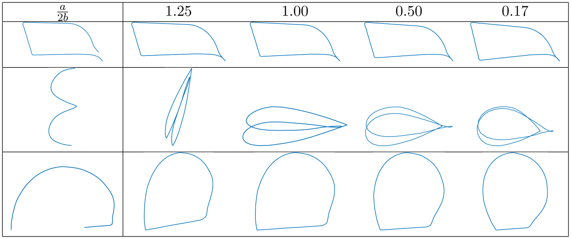
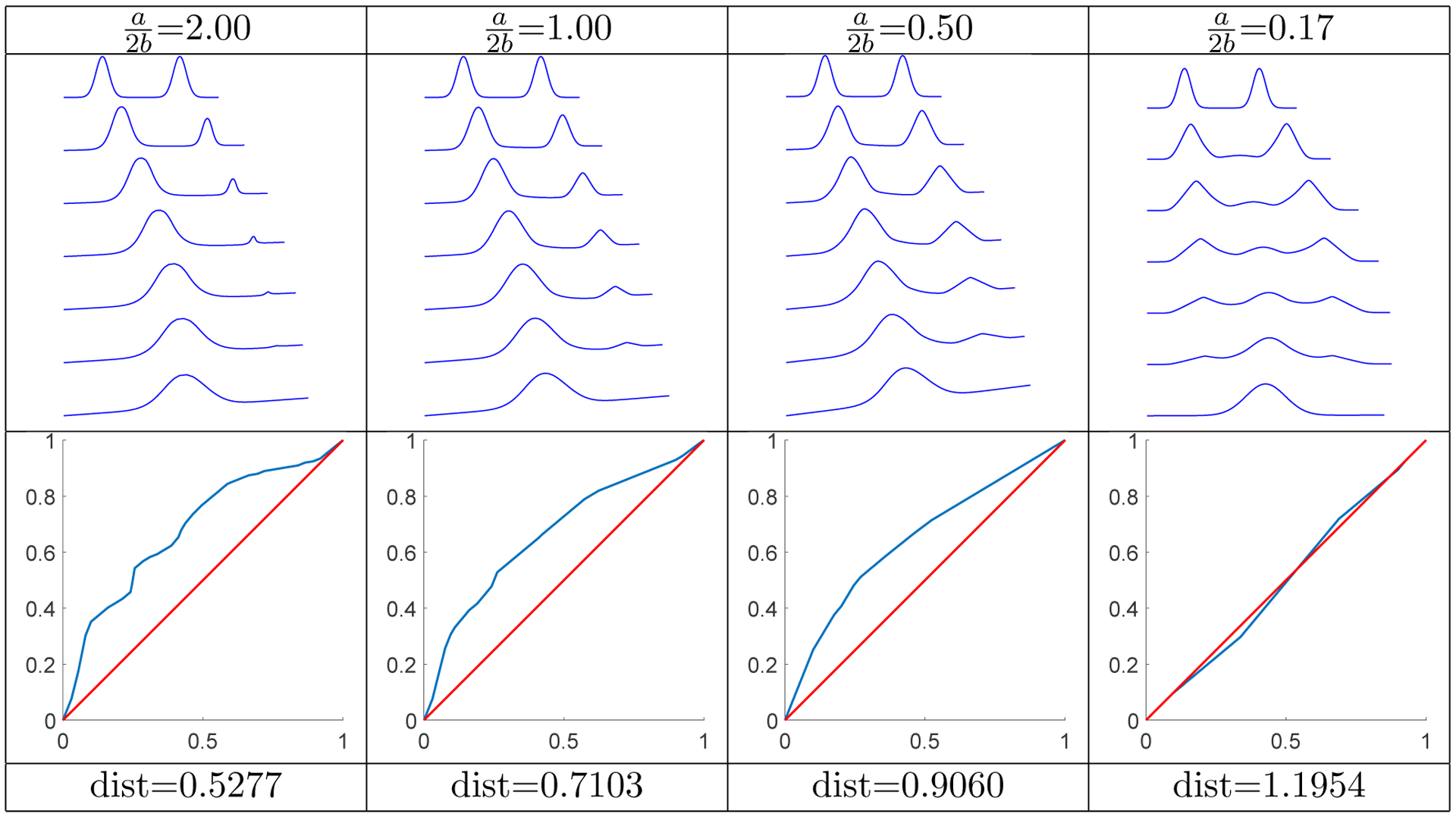
We show several examples of geodesic paths and associated geodesic distances between shapes of open (Figures 3–5) and closed (Figures 6 and 7) curves for different parameter values in the elastic metric, computed via the methods described in sections 4 and 6.1. Each figure shows the curve evolution and the optimal reparameterization in blue with the identity in red for comparison. While the example in Figure 3 considers two simulated open curves, the examples in Figures 4–7 use curves from the well-known MPEG-7 computer vision database.² Comparing within each figure shows the qualitative effect of parameter values on the curve evolutions, while comparing distances within shape classes across figures gives a sense of the range and distinguishing powers of the geodesic distance metrics. One can immediately make some qualitative observations. First, note that in each example the optimal reparameterizations for the $\frac{a}{2b}=0.5$ and 0.17 parameter choices are quite close to the identity. This was experimentally observed to be typical and makes sense heuristically: as the value of $\frac{a}{2b}$ is decreased, the penalty for stretching deformations in the elastic metric dominates, and bending deformations along the geodesic becomes less costly than reparameterizing to avoid them. Studying this behavior more quantitatively will be the subject of future work. Second, observe that distances increase as the ratio $\frac{a}{2b}$ is decreased. This is explained both by the higher penalty on reparameterizations (hence on matching similar features in the curves), as well as the fact that the (length normalized) curves lie on the Hilbert sphere $H_{a,b}^{\Sigma }(2b)$ after applying F_a,b (see Proposition 3.4). The figures were produced by fixing a = 1 and varying b, so that decreasing $\frac{a}{2b}$ corresponds to increasing the radius of the sphere containing their transformed images.

Figure 3.

Geodesic path and distance between shapes of two artificial open curves.

Figure 5.

Geodesic path and distance between two very different shapes.

Figure 6.

Geodesic path and distance between two very different shapes.

Figure 7.

Geodesic path and distance between two shapes of flowers with a different number of petals.

Figure 4.

Geodesic path and distance between two structurally different bone shapes.

We also provide a short classification experiment that shows the benefits of using general weights for the stretching and bending terms in the context of differentiating forgeries from genuine signatures. The data used here consists of 40 different signatures, which are a subset of the SVC 2004 dataset [51]. Each signature class contains 20 genuine signatures and 20 skilled forgeries. We classified each signature as genuine or a forgery using leave-one-out nearest neighbor with respect to the geodesic distance under the g^a,b metric for various parameter choices (a,b). As baselines, signatures were classified by two classical metric-based methods: L² distance between arclength parameterized curves, Hausdorff distance between the (discrete) arclength parameterized curves considered as unstructured point clouds, and Fréchet distance between the curves. Table 1 reports the overall classification rate (across all 40 signature classes) for each metric, as well as the number of signature classes where classification was perfect. The first group of three results contains parameter values covered by the R_a,b-transform of [5], with $\frac{a}{2b}=1$ corresponding to the SRVF and $\frac{a}{2b}=\frac{1}{2}$ corresponding to the complex square-root transform. The last three results are for parameter values obtained using our new transform. Classification is more successful for the parameter values given by our new results, with $\frac{a}{2b}=2$ matching the performance of the SRVF. Figure 8 shows the classification rates for $\frac{a}{2b}=1$ and $\frac{a}{2b}=2$ across the 40 individual signature classes. Although these parameter values have the same overall performance, we see that their performances differ drastically by signature class. This suggests that certain parameter values may be more sensitive to features appearing in particular signature classes, and that it is in general beneficial to vary the choice of parameters to suit a given task.

Table 1.

Overall classification rates and number of perfect classifications for the signature experiment.

Method	Classification rate	Perfect matches
Arclength	86.44	1
Hausdorff	90.81	3
Fréchet	91.75	3
$\frac{a}{2b}=\frac{1}{4}$	86.50	0
$\frac{a}{2b}=\frac{1}{2}$	93.81	6
$\frac{a}{2b}=1$	97.50	19
$\frac{a}{2b}=2$	97.50	19
$\frac{a}{2b}=3$	96.69	16
$\frac{a}{2b}=4$	97.00	16

Figure 8.

Classification rates across 40 individual signature classes using the geodesic distance for parameters $\frac{a}{2b}=1$ (in blue) and $\frac{a}{2b}=2$ (in red).

6.3. Complexity and runtime.

The computational complexity for computing distances between curves in shape space with any of the elastic metrics lies in the reparameterization step. The particular algorithm we are using, outlined in [40], enforces artificial constraints on the slope of each segment in the discrete reparameterization in order to improve speed. To match curves with n samples, the complexity of our algorithm is O(n²) (without the slope constraints, the complexity is O(n⁴)—see [40]). The runtime to compute geodesic distance between unparameterized open curves with n = 100 samples is on the order of hundredths of a second. For closed curves, the exhaustive seed search scales the runtime by a factor of n, but this can be improved for practical computations; e.g., one can compute L² distance between parameterized curves for all seed choices, then keep some smaller collection of best seeds to search over with dynamic programming. For $\frac{a}{2b}⩽1$, computing geodesics between registered curves is essentially instantaneous due to their explicit form for open curves under the F_a,b-transform and the fast projection algorithm for closed curves. When $\frac{a}{2b}>1$, the gradient-descent-based algorithm described in section 6.1 is employed to compute geodesics, and its runtime is highly dependent on parameter choices, which we have not optimized.

7. Future directions.

Our first direction for future work is to develop various statistical tools under this framework. These will include computation of summary statistics such as the average and covariance of a set of shapes, exploration of variability in various shape classes through PCA, building generative shape models, inference via hypothesis testing and confidence intervals, and finally regression analysis. Given the simplification of the metric under the proposed F_a,b-transform, and the simple geometry of the preshape space, we will be able to build upon existing work in this area based on the SRVF transform (i.e., $\frac{a}{2b}=1$) We have seen in the presented examples that different choices of a and b produce different geodesic paths, thus resulting in different statistical analyses.

Second, we will build statistical models that allow the data to choose appropriate values of a and b for the given application and task. For example, in the context of classification, one can learn optimal weights on training data and then apply the proposed framework on a held-out set. Furthermore, one can build hierarchical Bayesian models for registration, comparison, and averaging of shapes of planar curves that include priors on the values of a and b. Such models can be developed in a similar manner to the functional data approaches in [28, 32]. In those works, the authors simply work with fixed values of a and b. We propose to extend those methods by additionally including the weights for stretching and bending in the posterior distribution.

In previous work, one of the authors extended the results of Younes et al. [55] to give a metric with explicit geodesics on the space of closed loops in ${ℝ}^3$ [38]. This is accomplished by replacing the complex squaring map with the Hopf map S³ → S². Using quaternionic arithmetic, we expect that the results of this paper can be extended to provide transforms which simplify metrics on space curves as well.

REFERENCES

- [1].Anoshkina EV, Belyaev AG, and Seidel H-P, Asymptotic analysis of three-point approximations of vertex normals and curvatures, in Proceedings of Vision, Modeling, and Visualization, Aka GmbH, 2002, pp. 211–216. [Google Scholar]
- [2].Ayers B, Luders E, Cherbuin N, and Joshi SH, Corpus callosum thickness estimation using elastic shape matching, in International Symposium on Biomedical Imaging, 2015, pp. 1518–1521. [Google Scholar]
- [3].Bauer M, Bruveris M, Charon N, and M∅ller-Andersen J, A relaxed approach for curve matching with elastic metrics, ESAIM Control Optim. Calc. Var, 25 (2019), 72. [Google Scholar]
- [4].Bauer M, Bruveris M, Harms P, and M∅ller-Andersen J, A numerical framework for Sobolev metrics on the space of curves, SIAM J. Imaging Sci, 10 (2017), pp. 47–73, 10.1137/16M1066282. [DOI] [Google Scholar]
- [5].Bauer M, Bruveris M, Marsland S, and Michor PW, Constructing reparameterization invariant metrics on spaces of plane curves, Differential Geom. Appl, 34 (2014), pp. 139–165. [Google Scholar]
- [6].Bauer M, Bruveris M, and Michor PW, Why use Sobolev metrics on the space of curves, in Riemannian Computing in Computer Vision, Springer, 2016, pp. 233–255. [Google Scholar]
- [7].Bauer M, Harms P, and Michor PW, Almost local metrics on shape space of hypersurfaces in n-space, SIAM J. Imaging Sci, 5 (2012), pp. 244–310, 10.1137/100807983. [DOI] [Google Scholar]
- [8].Bauer M, Harms P, and Michor PW, Curvature weighted metrics on shape space of hypersurfaces in n-space, Differential Geom. Appl, 30 (2012), pp. 33–41. [Google Scholar]
- [9].Boyer DM, Lipman Y, Clair ES, Puente J, Patel BA, Funkhouser T, Jernvall J, and Daubechies I, Algorithms to automatically quantify the geometric similarity of anatomical surfaces, Proc. Natl. Acad. Sci. USA, 108 (2011), pp. 18221–18226. [DOI] [PMC free article] [PubMed] [Google Scholar]
- [10].Bronstein AM, Bronstein MM, Kimmel R, Mahmoudi M, and Sapiro G, A Gromov-Hausdorff framework with diffusion geometry for topologically-robust non-rigid shape matching, Int. J. Comput. Vis, 89 (2010), pp. 266–286. [Google Scholar]
- [11].Bruveris M, Optimal reparametrizations in the square root velocity framework, SIAM J. Math. Anal, 48 (2016), pp. 4335–4354, 10.1137/15M1014693. [DOI] [Google Scholar]
- [12].Bruveris M, Michor PW, and Mumford D, Geodesic completeness for Sobolev metrics on the space of immersed plane curves, in Forum of Mathematics, Sigma, Vol. 2, Cambridge University Press, 2014, e19. [Google Scholar]
- [13].Celledoni E, Eslitzbichler M, and Schmeding A, Shape analysis on Lie groups with applications in computer animation, J. Geom. Mech, 8 (2016), pp. 273–304. [Google Scholar]
- [14].Charon N and Trouvé A, The varifold representation of nonoriented shapes for diffeomorphic registration, SIAM J. Imaging Sci, 6 (2013), pp. 2547–2580, 10.1137/130918885. [DOI] [Google Scholar]
- [15].Charpiat G, Faugeras O, and Keriven R, Shape statistics for image segmentation with prior, in IEEE Computer Vision and Pattern Recognition, 2007, pp. 1–6. [Google Scholar]
- [16].Chazal F, Cohen-Steiner D, Guibas LJ, Mémoli F, and Oudot SY, Gromov-Hausdorff stable signatures for shapes using persistence, Computer Graphics Forum, 28 (2009), pp. 1393–1403. [Google Scholar]
- [17].Dryden IL and Mardia KV, Statistical Shape Analysis: With Applications in R, 2nd ed., Wiley, New York, 2016. [Google Scholar]
- [18].Duncan A, Klassen E, and Srivastava A, Statistical shape analysis of simplified neuronal trees, Ann. Appl. Stat, 12 (2018), pp. 1385–1421. [Google Scholar]
- [19].Glaunés J, Qiu A, Miller MI, and Younes L, Large deformation diffeomorphic metric curve mapping, Int. J. Comput. Vis, 80 (2008), pp. 317–336. [DOI] [PMC free article] [PubMed] [Google Scholar]
- [20].Gronwald F, On non-Riemannian parallel transport in Regge calculus, Classical Quantum Gravity, 12 (1995), pp. 1181–1189. [Google Scholar]
- [21].Haker S, Zhu L, Tannenbaum A, and Angenent S, Optimal mass transport for registration and warping, Int. J. Comput. Vis, 60 (2004), pp. 225–240. [Google Scholar]
- [22].Hamilton RS, The inverse function theorem of Nash and Moser, Bull. Amer. Math. Soc, 7 (1982), pp. 65–222. [Google Scholar]
- [23].Jermyn IH, Kurtek S, Klassen E, and Srivastava A, Elastic Shape Matching of Parameterized Surfaces Using Square Root Normal Fields, in European Conference on Computer Vision, Springer, 2012, pp. 804–817. [Google Scholar]
- [24].Joshi SH, Klassen E, Srivastava A, and Jermyn IH, A novel representation for Riemannian analysis of elastic curves in , in IEEE Computer Vision and Pattern Recognition, 2007, pp. 1–7. [DOI] [PMC free article] [PubMed] [Google Scholar]
- [25].Kendall DG, Shape manifolds, Procrustean metrics, and complex projective shapes, Bull. London Math. Soc, 16 (1984), pp. 81–121. [Google Scholar]
- [26].Klassen E, Srivastava A, Mio W, and Joshi SH, Analysis of planar shapes using geodesic paths on shape spaces, IEEE Trans. Pattern Anal. Mach. Intell, 26 (2004), pp. 372–383. [DOI] [PubMed] [Google Scholar]
- [27].Kriegl A and Michor PW, The Convenient Setting of Global Analysis, Math. Surveys Monogr 53, AMS, 1997. [Google Scholar]
- [28].Kurtek S, A geometric approach to pairwise Bayesian alignment of functional data using importance sampling, Electron. J. Stat, 11 (2017), pp. 502–531. [Google Scholar]
- [29].Kurtek S, Klassen E, Gore JC, Ding Z, and Srivastava A, Elastic geodesic paths in shape space of parametrized surfaces, IEEE Trans. Pattern Anal. Mach. Intell, 34 (2012), pp. 1717–1730. [DOI] [PubMed] [Google Scholar]
- [30].Laga H, Kurtek S, Srivastava A, Golzarian M, and Miklavcic SJ, A Riemannian elastic metric for shape-based plant leaf classification, in 2012 International Conference on Digital Image Computing Techniques and Applications (DICTA), 2012, pp. 1–7. [Google Scholar]
- [31].Lahiri S, Robinson D, and Klassen E, Precise matching of PL curves in in the square root velocity framework, Geom. Imaging Comput, 2 (2015), pp. 133–186. [Google Scholar]
- [32].Lu Y, Herbei R, and Kurtek S, Bayesian registration of functions with a Gaussian process prior, J. Comput. Graph. Statist, 26 (2017), pp. 894–904. [Google Scholar]
- [33].Mémoli F, Gromov–Wasserstein distances and the metric approach to object matching, Found. Comput. Math, 11 (2011), pp. 417–487. [Google Scholar]
- [34].Michor PW and Mumford D, Vanishing geodesic distance on spaces of submanifolds and diffeomorphisms, Doc. Math, 10 (2005), pp. 217–245. [Google Scholar]
- [35].Michor PW and Mumford D, An overview of the Riemannian metrics on spaces of curves using the Hamiltonian approach, Appl. Comput. Harmon. Anal, 23 (2007), pp. 74–113. [Google Scholar]
- [36].Miller MI and Younes L, Group actions, homeomorphisms, and matching: A general framework, Int. J. Comput. Vis, 41 (2001), pp. 61–84. [Google Scholar]
- [37].Mio W, Srivastava A, and Joshi S, On shape of plane elastic curves, Int. J. Comput. Vis, 73 (2007), pp. 307–324. [Google Scholar]
- [38].Needham T, Kähler structures on spaces of framed curves, Ann. Global Anal. Geom, 54 (2018), pp. 123–153. [Google Scholar]
- [39].Regge T, General relativity without coordinates, Nuovo Cimento (10), 19 (1961), pp. 558–571. [Google Scholar]
- [40].Robinson DT, Functional Data Analysis and Partial Shape Matching in the Square Root Velocity Framework, Ph.D. thesis, Florida State University, 2012. [Google Scholar]
- [41].Royden HL and Fitzpatrick P, Real Analysis, Vol. 2, Macmillan, New York, 1968. [Google Scholar]
- [42].Schumaker L, Spline Functions: Basic Theory, Cambridge University Press, 2007. [Google Scholar]
- [43].Small CG, The Statistical Theory of Shape, Springer, 1996. [Google Scholar]
- [44].Srivastava A, Klassen E, Joshi SH, and Jermyn IH, Shape analysis of elastic curves in Euclidean spaces, IEEE Trans. Pattern Anal. Mach. Intell, 33 (2011), pp. 1415–1428. [DOI] [PubMed] [Google Scholar]
- [45].Srivastava S, Lal SB, Mishra D, Angadi U, Chaturvedi K, Rai SN, and Rai A, An efficient algorithm for protein structure comparison using elastic shape analysis, Algorithms Molecular Biol, 11 (2016), 27. [DOI] [PMC free article] [PubMed] [Google Scholar]
- [46].Sundaramoorthi G, Yezzi A, and Mennucci AC, Sobolev active contours, Int. J. Comput. Vis, 73 (2007), pp. 345–366. [Google Scholar]
- [47].Trouvé A and Younes L, Diffeomorphic matching problems in one dimension: Designing and minimizing matching functionals, in European Conference on Computer Vision, 2000, pp. 573–587. [Google Scholar]
- [48].Trouvé A and Younes L, On a class of diffeomorphic matching problems in one dimension, SIAM J. Control Optim, 39 (2000), pp. 1112–1135, 10.1137/S036301299934864X. [DOI] [Google Scholar]
- [49].Tumpach AB and Preston SC, Quotient elastic metrics on the manifold of arc-length parameterized plane curves, J. Geom. Mech, 9 (2017), pp. 227–256. [Google Scholar]
- [50].Whitney H, On regular closed curves in the plane, Compositio Math, 4 (1937), pp. 276–284. [Google Scholar]
- [51].Yeung D, Chang H, Xiong Y, George S, Kashi R, Matsumoto T, and Rigoll G, SVC2004: First International Signature Verification Competition, in Biometric Authentication, 2004, pp. 16–22. [Google Scholar]
- [52].You Y, Huang W, Gallivan KA, and Absil P-A, A Riemannian approach for computing geodesies in elastic shape analysis, in Signal and Information Processing, 2015, pp. 727–731. [Google Scholar]
- [53].Younes L, Computable elastic distances between shapes, SIAM J. Appl. Math, 58 (1998), pp. 565–586, 10.1137/S0036139995287685. [DOI] [Google Scholar]
- [54].Younes L, Elastic Distance between Curves under the Metamorphosis Viewpoint, preprint, https://arxiv.org/abs/1804.10155, 2018. [Google Scholar]
- [55].Younes L, Michor PW, Shah JM, and Mumford DB, A metric on shape space with explicit geodesics, Atti Accad. Naz. Lincei Rend. Lincei Mat. Appl, 19 (2008), pp. 25–57. [Google Scholar]
- [56].Zahn CT and Roskies RZ, Fourier descriptors for plane closed curves, IEEE Trans. Comput, 21 (1972), pp. 269–281. [Google Scholar]