Quantification of Light Scattering Detection Efficiency and Background in Flow Cytometry

Knowledge of the sensitivity is essential for data interpretation and comparison between flow cytometers, especially when particles with signals close to the detection limit are studied, such as bacteria, extracellular vesicles, viruses, or other nanoparticles. For fluorescence, multiple methods have been developed to quantify sensitivity in terms of the detection efficiency Q and background light signal B (1, 2, 3, 4, 5, 6). All methods are based on the fact that light generates photoelectrons at the detector. Q is defined as the number of statistical photoelectrons generated at the detector per fluorochrome molecule passing through the illumination beam (4). B is the background light signal expressed in terms of the equivalent number of fluorochromes (4). The effect of different values of Q and B on the sensitivity of a flow cytometer has been described previously (4, 7). In short, a higher Q and a lower B increases the ability to resolve a dim population from the background noise.

Because scattered light also generates photoelectrons at the detector, it is theoretically possible to express the sensitivity of a light scatter detector in terms of Q and B as well. Currently, light scatter sensitivity is often expressed as the smallest detectable polystyrene (PS) bead, which thereby only specifies the detection threshold and provides no information about the ability to resolve dim populations (8). Expression of light scatter sensitivity in terms of Q and B would provide a more complete description of light scatter sensitivity. However, since flow cytometers provide data in arbitrary units (a.u.), a standardized unit is required to compare Q and B between different flow cytometers. In fluorescence, Q and B are commonly expressed in terms of molecules of equivalent soluble fluorophore (MESF), with Q in photoelectrons/MESF and B in MESF. A standardized unit that can be used to express and compare Q and B for light scatter was, hitherto, lacking. Recently, we explained how to use the scatter cross section (σ _s) in nm² as a standardized unit for scatter (9), which opened up the possibility of quantifying light scatter sensitivity in terms of Q and B. Here, we explore the feasibility of deriving Q and B to quantify light scatter sensitivity, using σ _s in nm² as the standardized unit.

Theory

The theory behind deriving Q and B for light scatter is similar to that for fluorescence (1, 2, 3, 4, 5). Detected signals are assumed to be linear with the light scattering power impinging the detector and dynode noise of the photomultiplier tube (PMT) is ignored. The theory below is derived in analogy to the derivation for fluorescence detectors as published by Chase and Hoffman (3).

Light scattered by a particle causes the generation of photoelectrons at the detector. For a constant signal, we define $\overline{n}$ as the mean number of photoelectrons generated at the detector. Because the emission of light is a stochastic process, the number of photons and the number of photoelectrons that are generated per time interval vary. This randomness in signal is known as photon noise (here), shot noise, or Poisson noise and affects both the signal originating from light scattered by a particle and the background originating from light scattered by other elements than the particle. Photon noise can be described by Poisson statistics, which results in a standard deviation of variations in optical signals:

$${\mathit{SD}}_{\text{phot.}}=\sqrt{\overline{n}}\left[-\right]$$ (1)

with units as specified in the square brackets. Please note that photoelectrons are elementary entities and not SI units and are therefore not reported between square brackets. To take into account the signal conversion and processing steps, such as the amplifier gain and the AD‐converter, $\overline{n}$ is related to a linear channel by gain factor G in a.u. per photoelectron, so that:

$${\mathit{SD}}_{\text{phot.}\text{meas.}}=G\sqrt{\overline{n}}\left[\mathrm{a}.\mathrm{u}.\right]$$ (2)

For light scattering, we assume that the mean scattered power P and $\overline{n}$ scale linearly with the total scattering cross section σ _s of a spherical particle in nm² (9):

$$P={\sigma }_s\left(d,n_p,n_m,\lambda \right)\bullet I_{\mathrm{ill}.}\left[\mathrm{W}\right]$$ (3)

where d is the particle diameter, n _p is the refractive index of the particle, n _m is the refractive index of the medium, λ is the wavelength of light in vacuum, and I _ill. is the illumination intensity in W/nm². For beads and flow cytometers d, n _p, n _m, and λ are known, so σ _s can be calculated with Mie theory (see Methods section). σ _s thereby is an intrinsic property of a bead and can thus be used as the standardized unit for light scatter. For reasons mentioned in the Discussion section, we neglect that P and $\overline{n}$ depend on the collection angles.

To relate σ _s to $\overline{n}$, we introduce the detection efficiency Q as the number of statistical photoelectrons per nm². Since the number of statistical photoelectrons scales linearly with illumination power, Q scales linearly with illumination power as well. Thus, after signal processing and in the absence of background, the mean signal of a particle and the corresponding standard deviation are given by:

$$\overline{S_{\mathrm{p}}}=G\overline{n_{\mathrm{p}}}=\mathit{GQ}{\mathrm{\sigma }}_{\mathrm{s}}\left[\mathrm{a}.\mathrm{u}.\right]$$ (4)

$${\mathit{SD}}_{\mathrm{p},\text{phot.}}=G\sqrt{\overline{n_{\mathrm{p}}}}=G\sqrt{Q{\mathrm{\sigma }}_s}\left[\mathrm{a}.\mathrm{u}.\right]$$ (5)

with $\overline{n_{\mathrm{p}}}$ is the mean number of photoelectrons generated by photons scattered from the particle. Thus, SD _p,phot. is associated with photon noise originating from light scattered by a particle, hereafter called particle photon noise. Similar to the scattering properties of a particle, also the background B can be expressed as the equivalent scattering cross section in nm² of a virtual particle required to produce the background. Here, we assume that B is dominated by background light originating from other sources than the particle and that electronic noise is negligible, which we experimentally confirmed in the Supporting Information Figure S6. In absence of a particle, the mean background signal and standard deviation after signal processing are then given by:

$$\overline{S_{\mathrm{B}}}=G\overline{n_{\mathrm{B}}}=\mathit{GQB}\left[\mathrm{a}.\mathrm{u}.\right]$$ (6)

$${\mathit{SD}}_{\mathrm{B},\text{phot.}}=G\sqrt{\overline{n_{\mathrm{B}}}}=G\sqrt{Q\mathrm{B}}\left[\mathrm{a}.\mathrm{u}.\right]$$ (7)

with $\overline{n_{\mathrm{B}}}$ is the mean number of photoelectrons generated by background photons. Thus, SD _B,phot. is associated with photon noise originating from light scattered by background elements, hereafter called background photon noise. The sum of Eqs. (4) and (6) results in the measured signal:

$$\overline{S_{\text{meas.}}}=\overline{S_{\mathrm{p}}}+\overline{S_{\mathrm{B}}}=G\overline{n_{\mathrm{p}}}+G\overline{n_{\mathrm{B}}}=\mathit{GQ}\left({\mathrm{\sigma }}_s+B\right)\left[\mathrm{a}.\mathrm{u}.\right]$$ (8)

The standard deviation of $\overline{S_{\text{meas.}}}$ involves SD _p,phot., SD _B,phot., variations in σ_s caused by intrinsic variations in the diameter and refractive index of a bead (SD _int), and variations in the uniformity of illumination of the sample stream (SD _ill.). Error propagation gives the following expression for the standard deviation of $\overline{S_{\text{meas}.}}$:

$${\mathit{SD}}_{\text{meas.}}=\sqrt{{{\mathit{SD}}_{\mathrm{p},\text{phot.}}}^2+{{\mathit{SD}}_{B,\text{phot.}}}^2+{{\mathit{SD}}_{\mathrm{int}.}}^2+{{\mathit{SD}}_{\mathrm{ill}.}}^2}\left[\mathrm{a}.\mathrm{u}.\right]$$ (9)

$\overline{S_{\mathrm{B}}}$ and SD _B,phot. can be determined for every illumination power from the measured background signals, that is, the signal obtained in absence of a particle. $\overline{S_{\text{meas}.}}$ and SD _meas. can then be corrected for the background:

$$\overline{S_{\text{meas.}\text{corr.}}}=\overline{S_{\text{meas.}}}-\overline{S_{\mathrm{B}}}=\overline{S_{\mathrm{p}}}\left[\mathrm{a}.\mathrm{u}.\right]$$ (10)

$${\mathit{SD}}_{\text{meas.}\text{corr.}}=\sqrt{{{\mathit{SD}}_{\text{meas.}}}^2-{{\mathit{SD}}_{\mathrm{B},\text{phot.}}}^2}=\sqrt{{{\mathit{SD}}_{\mathrm{p},\text{phot.}}}^2+{{\mathit{SD}}_{\mathrm{int}.}}^2+{{\mathit{SD}}_{\mathrm{ill}.}}^2}\left[\mathrm{a}.\mathrm{u}.\right]$$ (11)

The ratio of Eq. (11) to (10) gives the coefficient of variation (CV) of the background corrected signalCV _{meas. corr.}, which can be expressed as:

$${{\mathit{CV}}_{\text{meas.}\text{corr.}}}^2=\frac{{{\mathit{SD}}_{\text{meas.}\text{corr.}}}^2}{{\overline{S_{\text{meas.}\text{corr.}}}}^2}=\frac{{{\mathit{SD}}_{\mathrm{p},\text{phot.}}}^2+{{\mathit{SD}}_{\mathrm{int}.}}^2+{{\mathit{SD}}_{\mathrm{ill}.}}^2}{{\overline{S_{\mathrm{p}}}}^2}$$

$$=\frac{{{\mathit{SD}}_{\mathrm{p},\text{phot.}}}^2}{{\overline{S_{\mathrm{p}}}}^2}+\frac{{{\mathit{SD}}_{\mathrm{int}.}}^2+{{\mathit{SD}}_{\mathrm{ill}.}}^2}{{\overline{S_{\mathrm{p}}}}^2}={{\mathit{CV}}_{\mathrm{p},\text{phot.}}}^2+\frac{{{\mathit{SD}}_{\mathrm{int}.}}^2+{{\mathit{SD}}_{\mathrm{ill}.}}^2}{{\overline{S_{\mathrm{p}}}}^2}\left[-\right]$$ (12)

For a given population of beads measured at a relatively high illumination power, CV_p,phot. ² becomes negligible because the ratio of Eq. (5) to (4) converges to 0 for high $\overline{n_{\mathrm{p}}}$. Thus, for high illumination powers, Eq. (12) becomes:

$${{\mathit{CV}}_{\text{meas.}\text{corr.}\text{bright}}}^2={{\mathit{CV}}_{\mathrm{p},\text{phot.}}}^2+\frac{{{\mathit{SD}}_{\mathrm{int}.}}^2+{{\mathit{SD}}_{\mathrm{ill}.}}^2}{{\overline{S_{\mathrm{p}}}}^2}\approx \frac{{{\mathit{SD}}_{\mathrm{int}.}}^2+{{\mathit{SD}}_{\mathrm{ill}.}}^2}{{\overline{S_{\mathrm{p}}}}^2}\left[-\right]$$ (13)

Because SD _int., SD _ill., and $\overline{S_{\mathrm{p}}}$ scale linearly with illumination power, CV_{meas. corr. bright} is independent of illumination power. By varying the illumination power, we can thus study the stochastic process of scattered light at low illumination powers and determine the term SD _int. ² + SD _ill. ² at relatively high illumination powers. By combining Eqs. (12) and (13),

CV_p,phot. can be solved:

$${\mathit{CV}}_{\mathrm{p},\text{phot.}}=\sqrt{{{\mathit{CV}}_{\text{meas.}\text{corr.}\dim }}^2-{{\mathit{CV}}_{\text{meas.}\text{corr.}\text{bright}}}^2}\left[-\right]$$ (14)

where CV_{meas. corr. dim} is the background corrected CV of beads measured at relatively low illumination powers compared to CV_{meas. corr. bright} . Using Eqs. (4) and (5), CV_p,phot. can be expressed in terms of Q as follows:

$${\mathit{CV}}_{\mathrm{p},\text{phot.}}=\frac{{\mathit{SD}}_{\mathrm{p},\text{phot.}}}{\overline{S_{\mathrm{p}}}}=\frac{G\sqrt{Q{\mathrm{\sigma }}_{\mathrm{s}}}}{\mathit{GQ}{\mathrm{\sigma }}_{\mathrm{s}}}=\frac{\sqrt{G}\sqrt{\mathit{GQ}{\mathrm{\sigma }}_{\mathrm{s}}}}{\mathit{GQ}{\mathrm{\sigma }}_{\mathrm{s}}}=\frac{\sqrt{G}}{\sqrt{\mathit{GQ}{\mathrm{\sigma }}_s}}=\frac{\sqrt{G}}{\sqrt{\overline{S_{\mathrm{p}}}}}\left[-\right]$$ (15)

From Eq. (15), it follows that linear regression of CV_p,phot. versus $\frac{1}{\sqrt{\overline{S_{\mathrm{p}}}}}$ results in a slope J equal to $\sqrt{G}$, where we defined:

$$J\equiv \sqrt{G}\left[\sqrt{\mathrm{a}.\mathrm{u}.}\right]$$ (16)

In other words, J ² represents the measured signal in a.u. per statistical photoelectron. From Eq. (4), it follows that linear regression of σ_sversus $\overline{S_{\mathrm{p}}}$ results in a slope K equal to $\frac{1}{\mathit{GQ}}$, where we defined:

$$K\equiv \frac{1}{\mathit{GQ}}\left[\frac{{\mathrm{nm}}^2}{\mathrm{a}.\mathrm{u}.}\right]$$ (17)

K thereby relates the intrinsic bead property σ_s in nm² to the measured signal in a.u.. Substituting the definitions of J and K in Eqs. (15) and (4), we obtain the expressions:

$${\mathit{CV}}_{\mathrm{p},\text{phot.}}=\frac{J}{\sqrt{\overline{S_{\mathrm{p}}}}}\left[-\right]$$ (18)

$${\mathrm{\sigma }}_{\mathrm{s}}=K\bullet \overline{S_{\mathrm{p}}}\left[{\mathrm{nm}}^2\right]$$ (19)

Solving Eq. (15) for Q and filling in Eqs. (18) and (19) results in a practical expression for Q:

$$Q=\frac{1}{{{\mathit{CV}}_{\mathrm{p},\text{phot.}}}^2{\mathrm{\sigma }}_{\mathrm{s}}}=\frac{1}{\frac{J^2}{\overline{S_{\mathrm{p}}}}K\overline{S_{\mathrm{p}}}}=\frac{1}{J^{2}K}\left[\frac{1}{{\mathrm{nm}}^2}\right]$$ (20)

In turn, solving Eq. (7) for B and substituting G and Q using definitions (16) and (17) results in a practical expression for B as well:

$$B=\frac{{{\mathit{SD}}_{\mathrm{B},\text{phot.}}}^2}{G^{2}Q}={{\mathit{SD}}_{\mathrm{B},\text{phot.}}}^2\bullet \frac{1}{G}\bullet \frac{1}{\mathit{GQ}}={{\mathit{SD}}_{\mathrm{B},\text{phot.}}}^2\frac{K}{J^2}\left[{\mathrm{nm}}^2\right]$$ (21)

Factors affecting Q are I _ill (and thus the illumination power and illumination spot size), the acquisition time, the collection angle, the quantum efficiency of the detector, and the transmission efficiency of lenses and spectral filters (4). Factors affecting B include particles in the buffer, particles in the sheath and light scattering of optical components such as the flow cell wall.

Knowledge of Q and B allows determination of the separation S, which expresses the separation of dim light scatter signals and the background in terms of the number of standard deviations (4):

$$S=\frac{\sqrt{Q\bullet {\sigma }_s}}{\sqrt{1+2\bullet \frac{B}{{\sigma }_s}}}\left[-\right]$$ (22)

Lastly, using Q and B, the resolution limit (R), describing the lower limit at which light scatter signals can be fully discriminated from the background noise, can be calculated. R is the equivalent σ_s in nm² for which the standard deviation of the signal is separated from the standard deviation of the background noise (i.e., S = 2 in Eq. (22)) and can be calculated as follows:

$$R=\frac{2\left(\sqrt{2Q\bullet B+1}+1\right)}{Q}\left[{\mathrm{nm}}^2\right]$$ (23)

materials and methods

Materials

A bead mixture containing nonfluorescent NIST‐traceable PS bead populations with mean diameters of 100, 125, 147, 203, 296, 400, 600, 799, and 994 nm (all 3000 Series Nanosphere Size Standards; Thermo Fisher Scientific, Waltham, MA), and two green fluorescent bead populations of 140 and 380 nm, respectively (G140, G400; Thermo Fisher Scientific) was prepared in distilled water. The concentration of each bead population in the mixture was ~10⁷/ml.

Flow Cytometry

The side scatter (SSC) signal of the bead mixture was measured at illumination powers ranging from 20 mW to 200 mW for the 488 nm laser on a customized FACSCanto (10) (Becton Dickinson, Franklin Lakes, NJ). SSC collected on the customized FACSCanto is split by a dichroic mirror (NFD01‐488‐25x36; Semrock, Rochester, NY) and simultaneously detected by the standard SSC detection module and a high‐resolution SSC module (Supporting information Fig. S1). Data shown throughout this manuscript is the area parameter as measured by the standard SSC detection module with a fixed PMT voltage of 670 V. To ensure a reliable estimate of CV _{p. phot.}, we required particle photon noise to be the dominant (≥50%) source of the measured variation, which we could only achieve by selecting the standard SSC detection module together with illumination powers <100 mW and PS beads ≥400 nm. We selected the area parameter because in contrast to the height parameter, signals measured by the area parameter that are close to the detection limit scale linearly with the intensity of scattered light. See Supporting Information Figures S2–S4 and Table S1 for an analysis of the height parameter. For a complete description of the flow cytometer configuration, operating conditions and gating, please see the supplemented MIFlowCyt list.

The bead mixture was diluted 10‐fold in phosphate buffered saline (PBS, 21‐031‐CVR; Corning, Corning, NY) and measured at ~40 μl/min using a trigger on the high‐resolution SSC module (threshold of 200 a.u. at 267 V) to ensure detection of all beads. Per bead population, >1,000 events were acquired. To estimate SD _B,phot., the signal on the standard SSC channel was measured while triggering particles with a light scattering intensity ranging from 200 to 400 a.u., which is an order of magnitude below the detection limit of the standard SSC detection module, on the high‐resolution SSC module. We used this strategy to assure that the width of the sampling window, which affect the magnitude of the area parameter, is equal for beads and background signals. Figure S6 shows that SD _B,phot. versus illumination power can be well described by an allometric function and that electronic noise, which is represented by the offset of the fit, is negligible compared to the background photon noise.

Data Analysis

Median, robust standard deviation (rSD) and robust coefficient of variation (rCV) of the SSC area parameter were determined for all bead populations and the background signal. The rSD was defined as:

$$\mathrm{rSD}=\mathrm{½}\left({\text{percentile}}_{84.13}-{\text{percentile}}_{15.87}\right).$$

with percentile_84.13 and percentile_15.87 the measured signal of the bead population at those percentiles. The rCV was defined as the rSD divided by the median. Median, rSDs, and rCVs were preferred over the mean, SD and CV because they are less influenced by outliers and therefore more reproducible (4, 11). Data analyses were performed in MATLAB R2018b (Mathworks, Natick, MA).

Mie Theory

MATLAB scripts by Mätzler (12) were used to calculate σ_s integrated over all angles (4π), thereby taking into account the illumination wavelength (488 nm), the diameter and refractive index of each PS bead population (1.605 (13)) and the refractive index of PBS (1.339 (14)). In addition, σ_s was used to express R in terms of a bead diameter. Please read our earlier work (9) for alternative approaches and software to calculate σ_s.

results

Presence of Particle Photon Noise in the Signals

To allow derivation of Q and B, the variation caused by particle photon noise (CV _p,phot.) should have an observable contribution to CV _{meas. corr.}. In light scatter, the number of generated photoelectrons increases linearly with illumination power (Eq. (3)), thereby decreasing CV _p,phot. as described in Theory section. If CV _p,phot. has an observable contribution to CV _{meas. corr.}, a decrease in CV _{meas. corr.} is expected with increasing illumination power, since the intrinsic and illumination variations are constant over illumination power. To investigate whether this is the case, we measured the CV of four PS beads at different illumination powers.

Figure 1A shows CV _{meas. corr.} versus illumination power. A clear decrease in CV _{meas. corr.} is visible with increasing illumination power, indicating that CV _p,phot. has an observable contribution to CV _{meas. corr.} Because CV _p,phot. converges to 0 for large number of generated photoelectrons n, CV _{meas. corr.} converges to the intrinsic and illumination variations at illumination powers ≥100 mW. Hence, we limited the determination of Q and B to illumination powers <100 mW.

Figure 1.

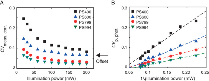
Presence of particle photon noisein light scatter. (A) Background corrected robust coefficient of variation (CV _{meas. corr.}) on side scatter versus illumination power for polystyrene (PS) beads of different diameters. CV _{meas. corr.} decreases with increasing illumination power, because detection of photons can be described by Poisson statistics. The remaining offset in CV _{meas. corr.} is due to intrinsic and illumination variations. (B) CV due to Poisson statistics (CV _p,phot.) versus 1/$\sqrt{\text{illumination power}}$ for different bead diameters (symbols). A linear relation can be fitted through all bead data (dashed lines, R ² > 0.96), confirming the presence of Poisson statistics in the signals. [Color figure can be viewed at wileyonlinelibrary.com]

Furthermore, since the number of generated photoelectrons is proportional to the illuminating power, CV _p,phot. is expected to scale linearly with $\frac{1}{\sqrt{\text{illumination power}}}$. Figure 1B shows that CV _p,phot. indeed scales linearly with $\frac{1}{\sqrt{\text{illumination power}}}$ for all beads (R ² > 0.96), thereby confirming the contribution of particle photon noise to the variation of measured signals.

Determination of Q and B

Now that particle photon noise has been confirmed, Q and B can be determined. Determination of Q and B consists of two steps: relating CV _p,phot. to $\overline{S_{\mathrm{p}}}$ in a.u. and in turn, relate $\overline{S_{\mathrm{p}}}$ to σ _s in standardized units of nm².

Figure 2A shows CV _p,phot. versus $\frac{1}{\sqrt{\overline{S_{\mathrm{p}}}}}$ which is linear for all illumination powers (R ² = 0.988) and results in slope J. Figure 2B shows σ_s versus $\overline{S_{\mathrm{p}}}$ and the linear regressions with slope K for the different illumination powers (R ² > 0.997). A subsequent plot of K versus illumination power (Fig. 2C) shows that K decreases with illumination power following a reciprocal relation (R ² = 0.996). Using this reciprocal relation, we extrapolated K at 200 mW. Now that factors J and K have been determined, Q, B and R can be calculated using Eqs. (20), (21), and (23). Table 1 shows the derived Q, B, and R at different illumination powers.

Figure 2.

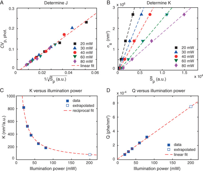
Deriving Q and B. (A) Measured robust coefficient of variation due to particle photon noise (CV _p,phot.) versus 1/$\sqrt{\overline{S_{\mathrm{p}}}}$ (symbols), with $\overline{S_{\mathrm{p}}}$ the background corrected median light scatter signal of 400, 600, 799, 994 nm polystyrene beads at different illumination powers. All data can be described by the linear fit (dashed line, R ² = 0.988) with slope J = 4.1 $\sqrt{a.u.}$. (B) Scattering cross section (σ_s) versus $\overline{S_{\mathrm{p}}}$ (symbols) of 400, 600, 799, 994 nm PS beads at different illumination powers. The slope of the linear fits (dashed lines, R ² > 0.997) represents the factor K per illumination power. (C) K versus illumination power. The data (symbols) can be described by a reciprocal relation (dashed line, R ² = 0.996), which was used to extrapolate K at 200 mW. (D) Q versus illumination power (symbols). As expected, Q increases linearly (dashed line, R ² = 0.999) with illumination power. [Color figure can be viewed at wileyonlinelibrary.com]

Table 1.

Q, B and R at different illumination powers

Illumination power	Q	B	R
(mW)	(1/nm2)	(nm2)a	(nm2)a	PS bead equivalent diameter (nm)
20	0.000073	2.99·105	2.12·105	472
30	0.00011	2.71·105	1.57·105	438
40	0.00015	2.49·105	1.27·105	415
60	0.00024	2.50·105	1.01·105	392
80	0.00032	2.38·105	8.38·104	375
200b	0.00074	2.73·105	5.70·104	342

PS: polystyrene.

^a Total scattering cross section.

^b Values at 200 mW are calculated using extrapolation of K.

Validation of Q, B, and R

Since the light scattering power, and there by the number of photoelectrons, increases linearly with illumination power (Eq. (3)), Q is expected to increase linearly with illumination power as well. Figure 2D shows that the relation between Q and illumination power is indeed linear with R ² = 0.999, indicating that the derived values for Q follow the expected trend.

Background level B is defined as the equivalent scattering cross section in nm² of a virtual particle required to produce the background. Thus, B is expected to be constant over illumination power. Table 1 indeed shows that B is similar (<26% difference) for all illumination powers and thus, as expected, independent of the illumination power.

The resolution limit R, as derived from Q and B (Eq. (23)), decreased with increasing illumination power. When comparing R with the measured side scatter histograms of the PS bead mixture (Fig. 3), R describes the limit from which light scatter signals can be fully discriminated from the background noise at 20 and 80 mW. At 200 mW, R corresponds to the detection of 342 nm PS beads, which seems an overestimation, because part of the 296 nm PS beads could be distinguished from the background noise. We attribute this overestimation due to the extrapolation required to calculate R at 200 mW (Fig. 2C,D).

Figure 3.

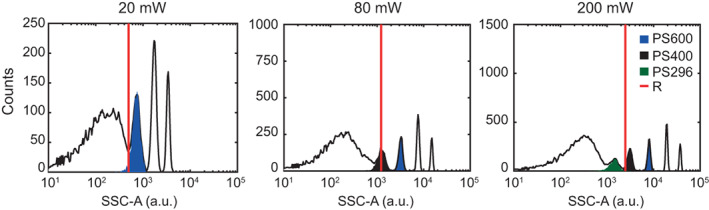
Side scatter histogram of a mixture of PS beads at 20, 80 and 200 mW as measured by the flow cytometer. The red solid line indicates R as calculated from Q and B and shown in Table 1. Bead populations can be clearly discriminated from the background noise for signals exceeding R. [Color figure can be viewed at wileyonlinelibrary.com]

discussion

Here, we explored the feasibility of deriving Q and B to quantify light scatter sensitivity. We found that particle photon noise contributes in a detectable way to the variation of light scatter signals measured by the SSC detector of a customized BD FACSCanto. We used Poisson statistics to quantify the number of statistical photoelectrons generated by light scattering of a particle. In combination with the scatter cross section σ _s in nm² as a standardized unit for light scatter, analysis of the particle photon noise allowed quantification of the light scatter sensitivity in terms of the efficiency Q in photoelectrons/nm² and background B in nm². Knowledge of Q and B allows derivation of the resolution limit R, which was found to describe the limit from which light scatter signals can be fully discriminated from the background noise.

Quantification of the number of statistical photoelectrons requires a measurement of the standard deviation resulting from the stochastic nature of light emission SD _p,phot.. The measured standard deviation SD _meas., however, also depends on intrinsic variations of the beads and on variations in the uniformity of illumination (Eq. (9)). In case of fluorescence, a bright fluorescent bead with a negligible CV _p,phot. is used to determine the contribution of intrinsic variations of the beads and variations in the illumination uniformity to SD _meas.. In turn, dim beads are used to determine SD _p,phot., assuming that the intrinsic variations of dim and bright fluorescent beads are similar (3, 4).

In case of scatter, however, intrinsic variations differ substantially between bead populations, which we attribute to differences in the CV of the size distributions of beads. Figure 4A shows that the CV of the mean diameter for PS beads of different sizes ranges from 0.008 for 799 nm beads up to 0.159 for 46 nm beads. Because the scattering cross section and thus light scattering intensities of the beads typically scale to the power of 4–6 with the diameter, intrinsic variations of bead populations often differ more than the CV of the bead diameter. As a result, the intrinsic variations of dim (i.e., small) and bright (i.e., large) beads in scatter differ and cannot be assumed to be similar. Hence, for scatter, a bright bead with negligible CV _p,phot. cannot be used to determine intrinsic and illumination variations.

Figure 4.

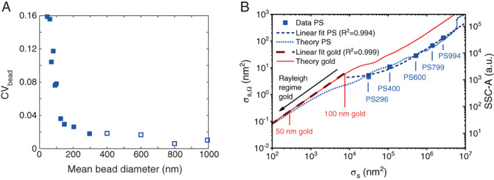
Bead limitations and requirements for deriving Q and B for scatter detectors. (A) Coefficient of variation on the mean bead diameter (CV _bead) versus mean bead diameter as derived from the mean and standard deviation specified by Thermo Fisher Scientific. Despite the relatively low CVs compared to polystyrene beads from other suppliers, CV _bead increases substantially with decreasing bead diameter, resulting in CVs for beads <200 nm that are twofold to eightfold larger than the CVs of the beads used in this work (open symbols). (B) Scattering cross section integrated over the collection angles of the used flow cyometer σ _s,Ω (left axis) and side scatter (right axis) versus total scattering cross section σ _s measured for PS beads (symbols) and calculated for polystyrene beads (short dots) and gold nanoparticles (line). Linear functions fit the datapoints (short dash, R ² = 0.994) and the theory of gold nanoparticles in the Rayleigh regime (long dash, R ² = 0.999) well. [Color figure can be viewed at wileyonlinelibrary.com]

Instead, we varied the illumination power and determined the intrinsic and illumination variations at the highest laser power (200 mW), assuming that CV _p,phot. becomes negligible. We found that only for illumination powers <100 mW and beads ≥400 nm, CV _meas. was dominated by CV _p,phot.. Therefore, we limited this study to illumination powers <100 mW. The downside of this approach is that determination of Q and B from CV_p,phot. at 200 mW, the operating illumination power of the flow cytometer, becomes impossible. To calculate Q and B at 200 mW, we extrapolated Q and B for lower illumination powers. The resulting R at 200 mW corresponds to the detection of 314 nm PS beads, which seems an overestimation, because part of the 296 nm PS beads could be distinguished from the background noise. We attribute this overestimation to the extrapolation required to calculate R at 200 mW (Fig. 2C,D).

Therefore, we do not recommend extrapolation of Q and B from low to relatively high illumination powers.

We found that B ranged from 2.38 to 2.99∙10⁵ nm² and was similar for all illumination powers (Table 1). In contrast to fluorescence, where B represents an actual background level and therefore increases with laser power, we defined B for scatter detectors as the equivalent scattering cross section in nm² of a virtual particle required to produce the background light scattering caused by elements other than the particle. B therefore represents an intrinsic property of elements causing background light scattering and is independent of the illumination power. From Eq. (3) follows that the power of the background signal scales linearly with illumination power. We further showed that background light scattering is the dominant source of variation in B, as for all illumination powers the standard deviation of the background photon noise is ≥37‐fold higher than the standard deviation of the electronic noise (Supporting Information Fig. S6).

The method described in this manuscript is applicable to scatter detectors of flow cytometers equipped with a laser with tunable output power and where particle photon noise is the dominant source of the measured variation. The SSC detector used in this study comprised a dichroic mirror that transmits only ~1% of the signal, thereby substantially reducing the signals and resulting in particle photon noise being the dominant source of variation. For common flow cytometers, particle photon noise can become the dominant source of variation by using PS beads <200 nm, but the CV on the mean diameter of current commercially available PS beads <200 nm is twofold to eightfold larger than the beads used in this work (Fig. 4A). A large CV on the mean diameter may cause the intrinsic variation to dominate CV _{meas. corr.}, thereby preventing an accurate determination of CV _p,phot., and leading to false Q and B values. Derivation of Q, B, and R for light scatter detectors of state‐of‐the‐art flow cytometers therefore requires reference particles that are dimmer than 200 nm PS beads and have a low CV (<2%).

Another disadvantage of the PS beads used in this work is that they do not scatter visible light isotropically. Although Figure 4B shows that we obtained a linear relation (R ² = 0.994) between the measured (and theoretical) light scattering intensity and the theoretical total scattering cross section σ _s, the relation is not necessarily linear for other flow cytometers with a different solid collection angle Ω. Although we can accurately calculate the angle‐weighted scattering cross section σ _s,Ω (9, 15) and account for the polarization of the illumination and polarization filters in front of the detector, we deliberately use σ_s for unpolarized illumination for three reasons. First, for a given illumination wavelength and medium, σ _s is an intrinsic property of the beads that is only dependent on the diameter and refractive index of the beads and the refractive index of the medium and thus independent of the used flow cytometer. Second, the goal of benchmark parameters Q,B, and R is to quantify the scatter sensitivity, which is affected by Ω, polarized illumination and polarization filters. Only by using σ _s instead of σ _s,Ω as a reference, benchmark parameters Q,B, and R do encompass Ω, polarized illumination and polarization filters. Third, because Ω differs between flow cytometers, σ _s,Ω differs between flow cytometer and would therefore not be a useful reference for future comparisons of the scatter sensitivity between flow cytometers.

Candidate reference particles to replace PS beads are 40–100 nm gold nanoparticles, which are dimmer and more monodisperse (16) than 200 nm PS beads and scatter light isotopically. Hence, gold nanoparticles may enable quantitation of Q, B, and R for scatter detectors of detectors that are more sensitive than our standard SSC detection module. The isotropic light scattering properties of gold nanoparticles (<100 nm) ensure a linear relationship between the measured light scattering intensity and σ _s, as shown in Figure 4B. Thereby, gold nanoparticles may extend the approach of Parks et al., who analytically described the variance versus mean signal intensities of optical pulses and beads to relate a.u. to photoelectron scales and quantify the background, from fluorescence to scatter detectors (6). Ideally, manufacturers of reference particles should not only report size characteristics, but in turn report the material and dispersion relation (the index of refraction as a function of wavelength) of both the reference particles and the medium, as well as the total scattering cross section at standard flow cytometry illumination wavelengths for the reference particles diluted in common buffers, such as water and PBS. If those reference particles (1) scatter light isotropically, (2) have a low CV on size (preferably <2%) and σ _s, and (3) have a traceably determined σ _s covering the detection range of the scatter detector, reference particles of different sizes and/or refractive indices can be combined to estimate Q, B, and R for scatter detectors.

Instead of beads, LED pulses could be used to relate a.u. to the number of statistical photoelectrons. However, our LED pulser (quantiFlash, APE Angewandt Physik & Elektronik GmbH, Berlin, Germany) has a dip in the output intensity at 488 nm (Supporting information Fig. S5), which together with the low transmission of the dichroic mirror disabled measuring signals over the entire range of the SSC detector. If a 488 nm LED pulser with a high output intensity would become available, it would be possible to directly relate the measured a.u. to the number of statistical photoelectrons, because LED pulses have little or no SD _int. and SD _ill. (Eq. (9)).

Although briefly mentioned by Steen (2), to our knowledge this is the first experiment to quantify the light scatter sensitivity of a flow cytometer in terms of Q and B. Knowledge of Q, B and the subsequent resolution limit R allows comparison of data from different flow cytometers, and comparison of flow cytometry data with data obtained using other techniques. Q, B and R are especially relevant when studying particles of which the light scatter signals are close to or below the background noise level. Furthermore, using the ability of Q and B to predict the separation S (Eq. (22)) between dim light scatter signals and the background, the accuracy of light scatter based sizing and refractive index determination can be derived (17, 18). Lastly, the possibility to monitor efficiency and background is useful in the design and development of flow cytometers.

In conclusion, we derived Q, B, and R for a scatter detector of a flow cytometer where particle photon noise is the dominant source of the measured variation. The approach is an important step toward quantification and standardization of light scatter detectors in flow cytometers and would improve substantially from the presence of monodisperse (CV < 2%) nanoparticles (<100 nm) that scatter light isotropically.

Author Contributions

Leonie de Rond: Conceptualization; methodology; original draft preparation; software; validation.Frank Coumans: Funding acquisition; writing‐review and editing. Joshua Welsh: Conceptualization; writing‐review and editing. Rienk Nieuwland: Writing‐review and editing. Ton van Leeuwen: Conceptualization; methodology; supervision; validation; writing‐review and editing. Edwin van der Pol: Conceptualization; funding acquisition; methodology; software; supervision; validation; writing‐review and editing.

CONFLICT OF INTEREST

F. A. W. Coumans and E. van der Pol are co‐founder and stakeholder of Exometry B.V., Amsterdam, The Netherlands. All other authors report no conflicts of interest.

Supporting information

AppendixS1: Supporting information

Supporting information 2

literature cited

- 1.Wood JC. Fundamental flow cytometer properties governing sensitivity and resolution. Cytometry 1998;33:260–266. [PubMed] [Google Scholar]
- 2.Noise SHB. Sensitivity, and resolution of flow cytometers. Cytometry 1992;13:822–830. [DOI] [PubMed] [Google Scholar]
- 3.Chase ES, Hoffman RA. Resolution of dimly fluorescent particles: A practical measure of fluorescence sensitivity. Cytometry 1998;33:267–279. [PubMed] [Google Scholar]
- 4.Hoffman RA, Wood JCS. Characterization of flow cytometer instrument sensitivity. Curr Protoc Cytom 2007;40:1.20.1–1.18. [DOI] [PubMed] [Google Scholar]
- 5.Gaucher JC, Grunwald D, Frelat G. Fluorescence response and sensitivity determination for ATC 3000 flow cytometer. Cytometry 1988;9:557–565. [DOI] [PubMed] [Google Scholar]
- 6.Parks DR, El Khettabi F, Chase E, Hoffman RA, Perfetto SP, Spidlen J, Wood JCS, Moore WA, Brinkman RR. Evaluating flow cytometer performance with weighted quadratic least squares analysis of LED and multi‐level bead data. Cytom Part A 2017;91A:232–249. [DOI] [PMC free article] [PubMed] [Google Scholar]
- 7.Wood JCS, Hoffman RA. Evaluating fluorescence sensitivity on flow cytometers: An overview. Cytometry. 1998;33:256–259. [PubMed] [Google Scholar]
- 8.Hoffman RA. Standardization, calibration, and control in flow cytometry. Curr Protoc Cytom 2005;32:1.3.1–3.21. [DOI] [PubMed] [Google Scholar]
- 9.de Rond L, Coumans FAW, Nieuwland R, van Leeuwen TG, van der Pol E. Deriving extracellular vesicle size from scatter intensities measured by flow cytometry. Curr Protoc Cytom 2018;86:e43. [DOI] [PubMed] [Google Scholar]
- 10.de Rond L, van der Pol E, Bloemen PR, Van Den Broeck T, Monheim L, Nieuwland R, van Leeuwen TG, FAW C. A systematic approach to improve scatter sensitivity of a flow cytometer for detection of extracellular vesicles. Cytom Part A 2020;97:582–591. [DOI] [PMC free article] [PubMed] [Google Scholar]
- 11.Shapiro HM. Data analysis. Practical Flow Cytometry. 4th ed.Hoboken, NJ: John Wiley & Sons, 2003; p. 235–236. [Google Scholar]
- 12.Mätzler C. MATLAB Functions for Mie Scattering and Absorption. Contract No.: 2002–08 Edn. Bern, Switserland: Institut für Angewandte Physik, University of Bern, 2002. [Google Scholar]
- 13.Kasarova SN, Sultanova NG, Ivanov CD, Nikolov ID. Analysis of the dispersion of optical plastic materials. Opt Mater. 2007;29:1481–1490. [Google Scholar]
- 14.Kindt JD. Optofluidic Intracavity Spectroscopy for Spatially, Temperature, and Wavelength Dependent Refractometry. Fort Collins, CO: Colorado State University, 2012. [Google Scholar]
- 15.Welsh JA, Horak P, Wilkinson JS, Ford VJ, Jones JC, Smith D, Holloway JA, Englyst NA. FCMPASS Software aids extracellular vesicle light scatter standardization. Cytometry A 2019;97:569–581. [DOI] [PMC free article] [PubMed] [Google Scholar]
- 16.Nanopartz Inc . Spherical gold nanoparticles. 2020. https://www.nanopartz.com/bare_spherical_gold_nanoparticles.asp (accessed 10 Aug 2020).
- 17.van der Pol E, de Rond L, Coumans FAW, Gool EL, Böing AN, Sturk A, Nieuwland R, van Leeuwen TG. Absolute sizing and label‐free identification of extracellular vesicles by flow cytometry. Nanomedicine. 2018;14:801–810. [DOI] [PubMed] [Google Scholar]
- 18.de Rond L, Libregts SFWM, Rikkert LG, Hau CM, van der Pol E, Nieuwland R, van Leeuwen TG, Coumans FAW. Refractive index to evaluate staining specificity of extracellular vesicles by flow cytometry. J Extracell Vesicles. 2019;8:1643671. [DOI] [PMC free article] [PubMed] [Google Scholar]
Associated Data
This section collects any data citations, data availability statements, or supplementary materials included in this article.
Supplementary Materials