3D‐Positioning of Nanoparticles in High‐Curvature Block Copolymer Domains

Abstract

The defined assembly of nanoparticles in polymer matrices is an important precondition for next‐generation functional materials. Here we demonstrate that a defined three‐dimensional nanoparticle assembly within the unit cells can be realized by directly linking the nanoparticles to block copolymers. We show that for a range of nearly symmetric to unsymmetric block copolymers there are only two formed structures, a hexagonal lattice of P6/mmm‐symmetry, where the nanoparticles are located in 1D‐arrays within the cylindrical domains, and a cubic lattice of Im3m‐symmetry, where the nanoparticles are located in the octahedral voids of a BCC‐lattice, corresponding to the structure of ferrite steel. We observe the block length ratio and thus the interfacial curvature to be the most important parameter determining the lattice type. This is rationalized in terms of minimal chain extension such that domain topologies with large positive curvature are highly preferred. Already volume fractions of only one percent are sufficient to destabilize a lamellar structure and favor the formation of highly curved interfaces. The study thus demonstrates how nanoparticles can be located on well‐defined positions in three‐dimensional unit cells of block copolymer nanocomposites. This opens the way to functional 3D‐nanocomposites where the nanoparticles need to be located on defined matrix positions.

By directly linking nanoparticles to block copolymers, defined three‐dimensional nanoparticle assemblies can be realized within domain unit cells. The block length ratio is the most important parameter determining the lattice type. Volume fractions of domains with large positive curvature of only one percent are already sufficient to destabilize lamellar structure and favor the formation of highly curved interfaces.

Introduction

The defined assembly of functional nanoparticles in polymer matrices is highly desirable for the development of next‐generation nano materials‐based devices.^[1] Currently, the lack of a precise control of nanoparticle position, distance and order in polymeric matrices is a severe barrier for many next‐generation materials as these parameters essentially determine mechanical, dielectric, magnetic or plasmonic coupling as well as energy transfer in the active matrices of the corresponding devices.

A versatile method to control nanoparticle location and assembly at the nanometer scale is the use of block copolymers.[², ³, ⁴, ⁵] For AB‐diblock copolymers it is possible to selectively deposit nanoparticles into the A‐ or B‐domains, or into the A/B‐interface.[⁶, ⁷, ⁸, ⁹, ¹⁰] Early studies aiming at a domain selective integration involved the synthesis of nanoparticles from precursors solubilized in the respective block copolymer domains, or used pre‐synthesized nanoparticles.[¹¹, ¹²] Later improved methods employed nanoparticles which were surface compatibilized with the targeted polymer domain.[¹³, ¹⁴] Surface compatibilization has recently been extended from linear to diblock copolymers, which opened a route to block copolymer nanocomposites, where the nanoparticles can be localized in the center of selected block copolymer domains. This has been demonstrated for polymer‐coated Au‐nanoparticles in thin films of bottle brush copolymers,^[15] for block copolymer‐coated iron oxide nanoparticles in micellar monolayers,[¹⁶, ¹⁷, ¹⁸] as well as for CuS nanoplatelets in PS‐P4VP^[19] and two‐dimensional assemblies.^[20]

For almost all applications of nanocomposites the 3D‐assembled structure is most relevant. Yet, the ordered and stoichiometric localization of nanoparticles within 3D‐block copolymer domains is still a challenge without the guidance of planar substrates or interfaces. Furthermore, it can have considerable complexity, as the incorporation of nanoparticles in diblock copolymers can lead to ternary phase systems with a structural variability comparable to ABC triblock copolymers.^[21]

In the present study we aimed for a controlled localization of nanoparticles in three dimensional domains of diblock copolymers. We focused on the interesting case where the nanoparticles are localized in the continuous domains which is relevant for all applications relying on nanoparticle coupling or nanoparticle‐mediated mechanical or transport properties. As a model system we chose nanocomposites consisting of iron oxide nanoparticles and poly(styrene‐b‐isoprene) diblock copolymers, where both the nanoparticles and the block copolymers can be synthesized with narrow size distribution on large scales.

For all investigated block lengths, nanoparticle diameters and grafting densities we remarkably found that only two phases, a hexagonal phase with P6/mmm‐symmetry, and a cubic phase with Im3m‐symmetry were formed. In the cubic phase the nanoparticles are localized in the octahedral voids of a BCC‐lattice, a structure which corresponds to the atomic Fe/C‐arrangement of ferrite steel.

Results and Discussion

For diblock copolymers the domain morphology is mainly determined by the domain volume fraction f. For our study we selected four different PS‐PI block copolymers that included a lamellae‐forming nearly symmetric diblock copolymer (HO‐PS₁₂₆‐PI₁₈₄, f _PS=0.48), a lamellae‐forming slightly asymmetric diblock copolymer (HO‐PS₁₇₁‐PI₁₃₈, f _PS=0.62) with a larger PS‐fraction, and a more asymmetric diblock copolymer (HO‐PS₂₄₈‐PI₁₀₂, f _PS=0.76) forming a hexagonal phase with PI‐cylinders in a PS‐matrix. The indices PS_n‐PI_m indicate the degrees of polymerization. These block copolymers all contain a terminal OH‐group at the PS‐block, which is functionalized with an amine to bind to the surface of the nanoparticles. To exclude block sequence specific effects, we also investigated the reverse case, a lamellae‐forming diblock copolymer (PS₁₂₃‐PI₂₀₇‐OH, f _PS=0.44) where the block copolymers attach to the nanoparticle surface via the PI‐blocks. The volume fractions f _PS of the neat block copolymers were calculated from the bulk densities and degrees of polymerization of the block copolymers as determined by SEC and ¹H‐NMR (Figures S15–S18) and for the nanocomposites using thermogravimetry to determine the nanoparticle weight fraction.

For the preparation of the nanocomposites we used iron oxide nanoparticles, which can be synthesized with narrow size distribution in high yields.^[22] Iron oxide nanoparticles with diameters between 4.6 and 8.0 nm were used for the investigation. The block copolymers were attached to the nanoparticle surface via strongly binding pentaethylene hexamine (PEHA) multidentate anchor groups. The block copolymers then form a stable and dense spherical polymer brush around the nanoparticle with either the PS‐blocks or the PI‐blocks as the inner layer. The attachment of the block copolymers was performed using a ligand exchange procedure.^[23] It allows to vary the grafting density of the block copolymers on the surface of the nanoparticles in a range from σ=0.16–1.20 chains nm⁻² by variation of the block copolymer concentration during the ligand exchange. The block copolymer‐grafted nanoparticles were carefully purified from oleic acid and unbound block copolymer ligands by selective precipitation steps as described in detail in ref. [23]. For each of the four diblock copolymers we prepared sets of nanocomposites with systematically varying grafting density and different nanoparticle diameters. Table 1 provides an overview of all block copolymers and nanocomposites investigated in the present study.

Table 1.

Structural parameters of the block copolymers and nanocomposites. The indices n, m in PS_n‐PI_m indicate the degrees of polymerization, D _NP is the diameter of the iron oxide nanoparticles, σ is the grafting density in polymer chains per nm², f _PI, f _PS, f _NP are the volume fractions of PI, PS, and nanoparticles, respectively, a are the unit cell dimensions, and D _dom the microdomain dimensions (lamellae, cylinder) derived from SAXS measurements. The volume fractions were calculated from the weight fractions using the bulk density of PS (ρ _PS=1.06 g cm⁻³), PI (ρ _PI=0.91 g cm⁻³) and Fe₂O₃ (ρ _PI=5.3 g cm⁻³).

	DNP [nm]	σ [nm2]	f PI	f PS	f NP	Phase	αSAXS [nm]	Ddom [nm]
PS126‐PI184			0.52	0.48	–	LAM	21.9	11.4
	5.5	0.16	0.46	0.42	0.12	P6/mmm
	5.5	0.36	0.50	0.45	0.06	P6/mmm
	4.6	1.20	0.52	0.47	0.01	P6/mmm	27.0
PS171‐PI138			0.38	0.62	–	LAM	20.3	6.2
	4.6	0.25	0.36	0.58	0.06	P6/mmm
	4.6	0.53	0.37	0.60	0.03	P6/mmm
	4.6	0.76	0.37	0.61	0.02	P6/mmm	26.3
	5.5	1.20	0.37	0.61	0.03	P6/mmm
PS248‐PI102			0.24	0.76		HEX	22.9	10.0
	8.0	0.60	0.23	0.74	0.03	Im3m	32.0
	8.0	0.80	0.23	0.74	0.03	Im3m	33.2
	4.6	1.01	0.24	0.75	0.01	Im3m	31.3
PS123‐PI207			0.56	0.44		LAM	18.3	9.9
	8.0	0.29	0.51	0.41	0.08	P6/mmm	31.3
	5.5	1.20	0.55	0.43	0.02	P6/mmm

The ordered morphologies of the neat diblock copolymers were characterized by small‐angle X‐ray scattering (SAXS) (Figure S1, see Supporting Information). The scattering curves all show a pronounced first maximum followed by a number of higher‐order reflections. PI₁₃₈‐PS₁₇₁‐OH, PI₁₈₄‐PS₁₂₆‐OH and PI₂₀₇‐PS₁₂₃‐OH form lamellar phases (LAM), whereas PI₁₀₂‐PS₂₄₈‐OH forms a hexagonally packed cylinder morphology (HEX). The suppression of the even reflections observed for PI₁₈₄‐PS₁₂₆‐OH and PI₂₀₇‐PS₁₂₃‐OH indicate that the diblock copolymers form almost perfectly symmetric lamellar domains.

In the following we describe the ordered morphologies formed by the nanocomposites derived from the four diblock copolymers. Whether the PS‐blocks or the PI‐blocks were attached to the nanoparticles is indicated by the sample identifiers, where Fe₂O₃@PS‐PI indicates attachment to the PS‐blocks and Fe₂O₃@PI‐PS indicates attachment to the PI‐blocks. All nanocomposites were prepared by casting solutions of the block copolymer coated nanoparticles from chloroform as a non‐selective solvent. A specially designed casting cell allows to delay the casting process to last over two weeks to provide sufficient time and polymer chain mobility to form ordered nanoparticle morphologies. The samples were subsequently annealed at 110 °C to remove traces of remaining solvent. The structures of the nanocomposites were characterized by SAXS as well as by electron microscopy on solvent‐cast thin films (TEM) and ultrathin sections of bulk nanocomposites (STEM).

Formation of a Hexagonal P6/mmm Structure

We will first discuss the morphologies formed by the slightly asymmetric lamellae‐forming PS₁₇₁‐PI₁₃₈ diblock copolymer. For the respective Fe₂O₃@PS₁₇₁‐PI₁₃₈ nanocomposites four different grafting densities covering a range from σ=0.25–1.2 nm⁻¹ with two different nanoparticle diameters (D _NP=4.6, 5.5 nm) were prepared. Figure 1 a shows the measured SAXS‐curves for the nanocomposites with grafting densities increasing from σ=0.25, 0.53 to 0.76 nm⁻². The scattering curves show a pronounced first order peak at q≈0.3 nm⁻¹, followed by several higher order peaks. The nanocomposite with the highest grafting density of σ=0.76 nm⁻² shows the highest order such that reflections up to 9^th order can be detected. The damped higher‐order peaks in the intermediate q‐range 0.4–0.9 nm⁻¹ envelope a weak q‐dependence which is close to q ⁻¹ as indicated by the straight line in Figure 1 a. Such a q‐dependence is characteristic for cylindrical structures or linear particle arrays. For q>1.5 nm⁻¹ we observe the Porod‐region with the characteristic q ⁻⁴‐scaling and the first form factor oscillation of the spherical nanoparticles. For spherical particles the position of the first minimum of the formfactor oscillation is given by q  R=4.493, such that from the position of the minima at q=1.6 and 2.0 nm⁻¹ nanoparticle radii of R=2.7 and 2.3 nm (D _NP=2R=5.5 and 4.6 nm) can be calculated, in good agreement with the values derived from TEM and compiled in Table 1. The scattering curve at the lowest grafting density shows an increased intensity at the onset of the Porod‐regime at q≈1.3 nm⁻¹ indicating nanoparticle multiplet formation similar as reported in 2D for low grafting densities.^[20]

Figure 1.

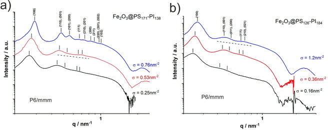
1D‐SAXS curves of the nanocomposites Fe₂O₃@PS₁₇₁‐PI₁₃₈ (a) and Fe₂O₃@PS₁₂₆‐PI₁₈₄ (b). Peaks are indexed as (hkl). For the nanocomposites the highest order is observed for the highest grafting densities where the first 9 reflections can be indexed on a hexagonal P6/mmm lattice.

For the nanocomposite with the highest grafting density of σ=0.76 nm⁻² the ratios for the positions of the 9 observed reflections is 1:1.73(√3):2:2.45(√6):2.65(√7):3:3.16(√10): 3.46(√12):3.61(√13). This agrees with the set of the first 9 reflections (hkl)=(100), (110/001), (200/101), (111), (210/201), (300), (211), (220/301/002), (102) of a 3D‐hexagonal lattice of space group P6/mmm having a ratio of unit cell dimensions of a=27.0 nm and c=a/2. For this lattice the reflection positions are given by $q_{hkl}=2\pi {\left(\frac{4}{3a^2}\left(h^2+hk+k^2\right)+\frac{l^2}{c^2}\right)}^{1/2}$ . For comparison, a hexagonally packed array of cylinders would result in a set of reflections with positions 1:1.73(√3):2:2.65(√7):3:3.46(√12) corresponding to the (hk)=(10), (11), (20), (21), (30) and (22) reflection. Thus, the observed 4^th (111), 7^th (211) and 9^th (102) reflection indicate the presence of a 3D hexagonal lattice. We will see below, that also all other nanocomposites prepared from symmetric or nearly symmetric block copolymers show the same structure.

An increasing order with increasing grafting density σ is generally observed for all nanocomposites in the present study. Higher grafting densities mediate stronger repulsive interactions between the nanoparticles such that they become localized on their lattice positions. The first order peak positions are shifted to lower q for lower grafting densities. This is on first instance counter intuitive, since lower grafting densities correspond to larger nanoparticle volume fractions. For a homogeneous distribution of nanoparticles this would lead to smaller inter‐particle distances, leading to peak shifts to higher q‐values. In the present case the nanoparticles form a linear array within cylindrical domains. It is already known from 2D‐studies[¹⁴, ²⁰] that lower ligand grafting densities reduce the distance between the nanoparticles. This is accompanied by a redistribution of ligand polymers from the inter particle region to the peripheral region of the cylindrical domains, which increases the inter cylinder distance. As the first order peak position is directly related to the inter cylinder distance, a concomitant shift to lower q‐values is observed. In line with this explanation based on the existence of cylindrical domains, for the Im3m‐lattice the low‐q shift of the first order peak at lower grafting densities is not observed (see Figure 4). For very low grafting densities the interparticle distance can become very small, facilitating multiplet formation, which leads to the increased intensity at q≈1.3 nm⁻¹ as describe above.

Figure 4.

a) 1D‐SAXS curves of the nanocomposites Fe₂O₃@PS₂₄₈‐PI₁₀₂. Peaks are indexed as (hkl). For the nanocomposites the highest order is observed for the highest grafting densities where the first 8 reflections on a cubic Im3m lattice can be detected. b) shows the measured 2D‐SAXS‐pattern of an oriented section of Fe₂O₃@PS₂₄₈‐PI₁₀₂, together with a 2D‐image calculated assuming the X‐ray beam to be parallel to the [100]‐direction of the Im3m crystal lattice (insert).

To further investigate the location of the nanoparticles in the block copolymer domains, we performed electron microscopy. Generally, bulk‐polymer sample preparation for electron microscopy requires microtoming to obtain ultrathin sections. In the case of polymer nanocomposites, ultramicrotoming can affect the nanoparticle distribution in the polymer domains due to the large difference in the hardness of nanoparticles and polymers. Therefore, we also prepared thin layers of the nanocomposites by solution casting on TEM‐grids followed by subsequent annealing for comparison.

In Figure 2 b we show a STEM‐micrograph of the ultrathin section of the nanocomposite sample recorded at a voltage of 30 kV using a scanning electron microscope SEM. Low‐voltage imaging in a SEM utilizes the much higher contrast between nanoparticles and block copolymers compared to high‐voltage transmission electron microscopes and gives a much better overview of the sample, because of the easy adjustable field of view. While very thin ultrathin sections have average thicknesses of ≈50 nm and because the nanoparticles have diameters of only ≈5 nm, even for the thinnest sections we image projections over many nanoparticle layers and unit cells. Still, ordered domains can be identified such as shown in Figure 2 b, where nanoparticles are arranged in parallel linear arrays. The distance between the arrays is d=13 nm, which well corresponds to the [110]‐projection of the P6/mmm lattice with a=27 nm≈2d as determined from SAXS.

Figure 2.

a) TEM‐image of a monolayer of Fe₂O₃@PS₁₂₆‐PI₁₈₄ showing the localization of the nanoparticles in PS cylindrical domains. b) STEM image of ultrathin section of a bulk Fe₂O₃@PS₁₇₁‐PI₁₃₈ nanocomposite showing the arrangement of the nanoparticles in the parallel assembled cylindrical microdomains. Also shown are calculations of the [100]‐projection (a) and the [210]‐projection (b) of nanoparticle arrays based on the P6/mmm unit cell with a=2c and a statistical mean deviations from the lattice points of δ=2.5 nm. Also shown are sets of unit cells visualizing the orientation for each particular projection.

Next, we consider the symmetric lamellae‐forming diblock copolymer PS₁₂₆‐PI₁₈₄ with a PS‐volume fraction of f _PS=0.48. For this block copolymer a series of Fe₂O₃@PS₁₂₆‐PI₁₈₄‐nanocomposites with varying grafting densities from σ=0.16, 0.36 and 1.20 nm⁻² were prepared. As seen in Figure 1 b, for the Fe₂O₃@PS₁₂₆‐PI₁₈₄ nanocomposites we observe very similar scattering curves as for the Fe₂O₃@PS₁₇₁‐PI₁₃₈ nanocomposites. The highest order is again observed for the highest grafting density, where the first‐order peak is clearly resolved together with damped higher‐order reflections. The presence of the (210)/(021)‐peaks is a strong indication for the formation of the P6/mmm‐lattice, albeit the peak widths are larger compared to the Fe₂O₃@PS₁₇₁‐PI₁₃₈ nanocomposites. At intermediate q‐values we again observe a q ⁻¹‐envelope characteristic for cylindrical structures or linear nanoparticle arrays. The well‐observable form factor minima are located at q=1.6 and 1.9 nm⁻¹, corresponding to radii of R=2.8 nm and 2.3 nm (d=5.5 and 4.6 nm) in agreement with the values determined by TEM (see Table 1). Also here for the lowest grafting density a slight upturn is observed at q=1.05 nm⁻¹ indicating the formation of nanoparticle multiplets.

Figure 2 a shows a TEM‐micrograph of a solution‐cast Fe₂O₃@PS₁₂₆‐PI₁₈₄‐nanocomposite monolayer. The PI domains were stained by OsO₄ and appear grey between the white PS domains and the black iron oxide nanoparticles. We clearly observe that the nanoparticles are located in the PS‐domains and that the internanoparticle distance d _NP=13.6 nm again is half the intercylinder distance d _cyl, in agreement with the c=a/2 relation derived form the Bragg‐peak positions in the measured SAXS‐curves for the P6/mmm‐lattice. We can conclude that for symmetric and unsymmetric lamellae‐forming diblock copolymers irrespective of the block lengths, the nanoparticle diameter or the grafting density we observe the same hexagonal morphology, which for the highest ordered nanocomposites can be determined to have a P6/mmm‐structure.

From the simulations of the STEM‐images (Figure 2) and from model fits of the scattering curves (Figure S7) we determined the mean square displacement of the nanoparticles from their ideal lattice position to be δ=2.5–3 nm, which is slightly smaller than the diameter of the nanoparticles. This is a reasonable positional fidelity for many applications. Yet, we observe that the relative spatial distribution appears to be non‐Gaussian, and rather evenly spread around the ideal lattice point. This gives rise to the rather unusual random distribution of the nanoparticles around their lattice points as observed by STEM, and to the observation of many higher order reflections, even if the peak widths are rather broad.

Figure 3 a shows the proposed structure for the nanocomposites Fe₂O₃@PS₁₇₁‐PI₁₃₈ and Fe₂O₃@PS₁₂₆‐PI₁₈₄. It consists of hexagonally arranged cylindrical domains, within which the nanoparticles are ordered in linear arrays. The nanoparticle distance d _NP is half the distance between the cylinders d _cyl, which is equal to the lateral dimension a of the unit cell. The arrangement of the nanoparticles within the unit cells keeps the mmm‐symmetry and is thus compatible with the P6/mmm space group and the corresponding reflections observed in SAXS. In the Supporting Information we show in detail (Figures S8, S9) that all polymer domain sizes in both unit cells shown in Figure 3 are consistent with the mean‐square end‐to‐end distance of the polymer blocks.

Figure 3.

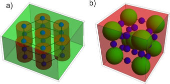
a) Representation of the P6/mmm lattice with the nanoparticles (blue) arranged in a linear array within the PS‐cylinders (red) in the PI‐matrix (green). The structure represent a relative cylinder radius R _cyl/a=0.37 and a relative nanoparticle radius of R _NP/a=0.12 to agree with the relative sizes and the volume fractions of the nanocomposite Fe₂O₃@PS₁₇₁‐PI₁₃₈. b) Representation of the Im3m lattice with the nanoparticles (blue) arranged in the octahedral voids of a BCC lattice consisting of PI‐spheres (green) in a PS‐matrix (red). The structure represents a relative PI sphere radius of R _sph/a=0.30 and a relative nanoparticle radius of R _NP/a=0.11 to agree with the relative sizes and the volume fractions of the nanocomposite Fe₂O₃@PS₂₄₈‐PI₁₀₂.

Formation of a Cubic Im3m Void Structure

Next, we consider the block copolymer PI₁₀₂‐PS₂₄₈ with the highest PS‐volume fraction of f _PS=0.76. The neat block copolymer forms a morphology with PI‐cylinders that are hexagonally arranged in a continuous PS‐matrix. We prepared a series of Fe₂O₃@PS₂₄₈‐PI₁₀₂‐nanocomposites with grafting densities ranging from σ=0.6, 0.8 to 1.0 nm⁻².

The measured scattering curves are shown in Figure 4 a for the grafting densities σ=0.6, 0.8 and 1.01 nm⁻². Also for this system we observe a strong first‐order peak together with a set of higher‐order reflections. In the intermediate q‐region, the higher‐order reflections are enveloped by a q ⁰‐dependence indicated by the dashed line, which is characteristic for the Guinier‐regime of spherical objects. The position of the formfactor minimum is at q=1.15 and 1.9 nm⁻¹, corresponding to nanoparticle radii of R=4.0 and 2.3 nm (diameters of 8.0 and 4.6 nm), in agreement with values derived from TEM and collected in Table 1. For the sample with the highest grafting density the ratio of the reflection positions is 1:1.41(2):1.73(√3):2:2.24(√5):2.45(√6):2.64(√7):2.82(√8) well corresponding to the set of the first eight (hkl)=(110), (200), (211), (220), (310), (222), (321), (400) reflections of the BCC‐lattice with space group Im3m. The peak positions for this space group are given by $q_{hkl}=\frac{2\pi }{a}{\left(h^2+k^2+k^2\right)}^{1/2}$ with the unit cell size of a=31.3 nm. Higher grafting densities mediate stronger repulsive interactions between the nanoparticles such that they become localized on their lattice positions. This particularly applies to the nanoparticles in the octahedral voids of the Im3m‐lattice. We observe that the lower grafting densities lead to lower degree of order with a smaller number of reflections.

Figure 4 b shows the measured 2D‐SAXS‐pattern for an oriented section of the Fe₂O₃@PS₂₄₈‐PI₁₀₂‐nanocomposites. Oriented regions of several hundred micrometers are observed close to the sample surface, where during slow solvent evaporation uniform lattice orientations are induced by the presence of the substrate surfaces. On the meridian we can resolve the set of (101)‐ and (202)‐reflections, together with the off‐meridian (200) and (310) reflections. The observed peak positions are in agreement with the Im3m‐diffraction pattern assuming the X‐ray beam to be parallel to the [100]‐direction. This is shown by the calculated 2D‐pattern displayed in the insert in Figure 2 b. The vertical peak broadening of the off‐meridian reflections is due to an orientational distribution around the [100]‐direction.

To determine the position of the nanoparticles in the BCC‐lattice we performed STEM at low acceleration voltages an ultrathin sections, as well as TEM on solvent‐cast monolayers. Figure 5 a) shows a TEM‐image of a monolayer featuring a square arrangement of nanoparticles of alternating dark and grey intensity. This pattern agrees well with the simulated pattern for the [100]‐projection of the BCC‐lattice with the nanoparticles occupying the octahedral voids. The indicated unit cell size of a=d ₁₀₀=31 nm well agrees with the value of 31.3 nm determined by SAXS. The structure of the unit cell is shown in Figure 3 b with its respective orientation in Figure 5 a. The PI‐spheres in the PS‐matrix are located at the (0,0,0)‐ and (1/2,1/2,1/2)‐positions of the unit cell. The low‐voltage STEM‐image of an ultrathin section in Figure 5 b shows crossed linear arrays of nanoparticles enclosing white rectangular areas corresponding to the positions of the PI‐spheres, which are indicated by red circles. This pattern is characteristic for a projection of a thin section oriented in [110]‐direction. The long distance between the centers of the white areas is d ₁₀₀=33 nm, and the short distance is d ₁₁₀=23 nm, which is $\frac{d_{100}}{\sqrt{2}}\approx 24$  nm in agreement with the BCC‐lattice. The respective orientation of the unit cell is indicated in Figure 5 b. Figure 5 c shows a STEM‐image of an ultrathin section featuring linear nanoparticle arrays encircling hexagonally arranged white domains characteristic for a thin section oriented in [111] direction. The mean distance between the white domains is d ₁₀₀=20.8 nm which is $\frac{d_{100}}{\sqrt{3}}\sim 20$  nm in agreement with the BCC lattice. The corresponding to the orientation of the unit cell shown in Figure 5 c. Finally, the STEM‐image of an ultrathin section in Figure 5 d shows parallel linear arrays of nanoparticles characteristic for oblique orientation close to the [x10]‐orientation with x≈2. The interline distances is d=18 nm, which agrees well with d ₁₁₀/2=18.5 nm. For all STEM‐images in Figure 5 we performed the simulations with a mean deviation of δ=3 nm from the ideal lattice point to take into account the positional disorder of the nanoparticles.

Figure 5.

a) TEM‐image of monolayers showing the arrangement of the nanoparticles in the cubic microdomains of Fe₂O₃@PS₂₄₈‐PI₁₀₂ nanocomposite. b), c), d) STEM‐images at 20 kV showing arrangements of nanoparticles in ultrathin sections of the nanocomposites in [110] b), [111] c), and an oblique [x10] direction d). Simulated images based on a BCC lattice with the nanoparticles located within the octahedral voids are shown, together with the unit cell to visualize the corresponding orientation. The statistical mean deviations from the lattice points is δ=3.0 nm. The red circles indicate the positions of the PI‐spheres. White rectangles indicate characteristic projections in the electron microscopy images.

Notably, we observe this Im3m‐structure with the nanoparticles occupying the octahedral voids of a BCC‐lattice (BCC_void) for all grafting densities and for the two different nanoparticle diameters investigated. Interestingly, the observed location of the nanoparticles in the octahedral voids corresponds to the structure of ferrite steel, where the carbon atoms are located in the octahedral voids of the iron BCC‐lattice. The octahedral voids are located in the center of the 6 faces of the BCC unit cell and in the center of all 12 edges of the unit cell. Thus there are 6 octahedral voids per unit cell. There are also tetrahedral voids located on the center of the faces of the BCC unit cell. Simulations shown in the Supporting Information (Figures S11–S13) demonstrate, that the corresponding projections do not agree with the observed STEM images.

Finally, we investigated the PI₂₀₇‐PS₁₂₃‐diblock copolymer, where the PI‐blocks were bound to the nanoparticle surface. The pure block copolymers is nearly symmetric with a PS volume fraction of f _PS=0.44 forming a lamellar phase. Fe₂O₃@PI₂₀₇‐PS₁₂₃ nanocomposites with two different grafting densities were prepared with σ=0.29 and 1.2 nm⁻². The measured scattering curves are shown in Figure S5 in the Supporting Information. Also for Fe₂O₃@PI₂₀₇‐PS₁₂₃ at the highest grafting densities we observe scattering curves characterized by a pronounced first reflection and a set of damped higher‐order reflections. Again, there is a q ⁻¹‐envelope at intermediate q, and a formfactor oscillations. The positions of the formfactor minima at q=1.1 and 1.6 nm⁻¹ correspond to R=4.0 nm and 2.8 nm (diameter 8.0 and 5.5 nm) in agreement with the values in Table 1. The higher‐order reflections are broadened, but are compatible with the hexagonal peak positions for the P6/mmm‐structure observed for the other nanocomposites. This demonstrates, that also in the inverse case the nanoparticles induce hexagonal domain structures with large interfacial curvature, even for nearly symmetric block copolymers. In the case of Fe₂O₃@PI₂₀₇‐PS₁₂₃ the nanoparticles are located in the PI‐cylinders, which are embedded in a PS‐matrix. This can also well be observed from the TEM‐images, where the nanoparticles are embedded in the stained PI‐domains (Figure S6 in Supporting Information).

Superlattice Topology and Interfacial Curvature

Generally, the incorporation of nanoparticles in diblock copolymers domains will increase their volume fraction which can lead to changes in the domain morphology. In our case, the incorporation of nanoparticles into the PS‐domains of the lamellae‐forming PS‐PI‐diblock copolymers would be expected to lead a PS‐matrix phase embedding PI‐cylindrical or spherical domains. In our study the opposite is observed, that is, the Fe₂O₃@PS₁₂₆‐PI₁₈₄ and Fe₂O₃@PI₁₇₁‐PS₁₃₈ nanocomposites both form a PI‐ matrix phase containing PS‐cylindrical domains with embedded nanoparticles. The same is true for Fe₂O₃@PI₂₀₇‐PS₁₂₃, where PI‐cylinders with embedded nanoparticles are formed, although the neat block copolymer forms a lamellar phase and the addition of PI‐embedded nanoparticles should have led to the formation of PS‐cylinders in a PI‐matrix. These changes in the morphologies are observed for nanoparticle particle volume fractions as low as f=0.01.

Thus, for the nanocomposites we observe a very strong tendency to form ordered assemblies with large positive interfacial curvature. This facilitates the accommodation of the local spherical geometry of the polymer brush surrounding the nanoparticles. Therefore the nanoparticles are localized within the cylinders of the P6/mmm‐lattice or within the octahedral voids of the Im3m‐lattice. Remarkably, we observe only these two lattices for the set of diblock copolymers over volume fractions of f _PS=0.44–0.76, for grafting density over a range from σ=0.16–1.5 and for three different nanoparticle diameters. We find that a variation of the grafting density only affects the degree of order, not the lattice type.

To rationalize the occurrence of these two lattice‐types we compare our results on bulk 3D‐nanocomposites with recent results on 2D nanocomposite monolayers.^[20] For the 2D‐system there is a transition from I‐stripe domains with linear arrangements of nanoparticles to honeycomb domains with Y‐connected linear arrangements of nanoparticles on a planar surface. The stripe → honeycomb transition parallels the P6/mmm → BCC_void transition observed in the present study (Figure 6 a,c), which involves a transition from I‐stripe domains with linear arrangements of nanoparticles to X‐connected arrangements of nanoparticles in the octahedral voids on the planar surface of the unit cell when viewed from the [100]‐direction. In 2D this sequence is driven by minimizing the polymer chain extension resulting from connecting the nanoparticle surface to the domain interface as indicated in Figure 6 b. The degree of extension depends on the grafting density σ and the nanoparticle/domain size ratio d/D such that higher grafting densities and higher ratios d/D favor the transition from I‐ to Y‐nanoparticle arrangements as in the stripe → honeycomb transition.

Figure 6.

Scheme of a) the linear array → honeycomb lattice transition observed in 2D and the c) P6/mmm → BCC_void transition observed in 3D. The honeycomb lattice features Y‐connected nanoparticles in a planar surface. The BCC_void lattice features X‐connected nanoparticles on the planar surface of the BCC unit cell. b) and d) specify the geometrical parameters that determine the stretching of the polymer chains to connect the nanoparticle surface to the interface.

As outlined above, we observe for 3D assemblies that the interfacial curvature C is the most important factor determining the lattice type. We therefore adapt the model established for 2D‐systems on polymer chain stretching as a function of grafting density and size ratio d/D to 3D‐systems as a function of interfacial curvature.^[24] Figure 5 b shows that a polymer chain is extended by a factor α _max=D/(2a) to connect the nanoparticle surface to the domain interface. As shown in Figure 6 d, for a strongly curved interface with a curvature C=1/R and a curvature radius of R=2D the extension factor is given by α _max=1/(C  a). An increasing curvature C will therefore reduce the maximum chain extension. Therefore, lamellar with planar interfaces having C=0 or interfaces with locally negative curvature C<0 will be highly unfavorable, whereas interfaces with large positive curvature like for cylindrical interfaces in P6/mmm or spherical interfaces in BCC will be strongly preferred. A more detailed description requires the use of recently developed atomistic, course‐grained and field‐based simulation techniques that proved to be successful in the prediction of polymer nanocomposite morphologies.[²⁵, ²⁶]

Conclusion

We demonstrate the stoichiometric three‐dimensional localization of nanoparticles within the domains of diblock copolymer nanocomposites. We further show that for a range of nearly symmetric to asymmetric block copolymers there are only two formed structures, (i) a hexagonal lattice of P6/mmm‐symmetry, where the nanoparticles are located in 1D‐arrays within cylindrical domains, and (ii) a cubic lattice of Im3m‐symmetry, where the nanoparticles are located in the octahedral voids of a BCC‐lattice. This nanoparticle superlattice corresponds to the lattice of carbon atoms in ferrite steel. We generally find that increasing the grafting density increases the degree of order. We observe the block length ratio and thus the interfacial curvature to be the most important parameter determining the lattice type. This is rationalized in terms of minimal chain extension such that domain topologies with large positive curvature are highly preferred. Already volume fractions of only one percent are sufficient to destabilize lamellar structure and favor the formation of highly curved interfaces.

The study thus demonstrates how nanoparticles can be located on well‐defined positions in three dimensions within the domains of block copolymer nanocomposites. This opens the way for to functional 3D‐nanocomposites where the nanoparticles need to be located on defined positions, where in addition macroscopic domain orientation is possible.

Conflict of interest

The authors declare no conflict of interest.

Supporting information

As a service to our authors and readers, this journal provides supporting information supplied by the authors. Such materials are peer reviewed and may be re‐organized for online delivery, but are not copy‐edited or typeset. Technical support issues arising from supporting information (other than missing files) should be addressed to the authors.

Supporting Information

V. B. Leffler, S. Ehlert, B. Förster, M. Dulle, S. Förster, Angew. Chem. Int. Ed. 2021, 60, 17539.

References

- 1.Boles M. A., Engel M., Talapin D. V., Chem. Rev. 2016, 116, 11220–11289. [DOI] [PubMed] [Google Scholar]
- 2.Balasz A. C., Emrick T., Russell T. P., Science 2006, 314, 1107–1110. [DOI] [PubMed] [Google Scholar]
- 3.Bockstaller M. R., Mickiewicz R. A., Thomas E. L., Adv. Mater. 2005, 17, 1331–1349. [DOI] [PubMed] [Google Scholar]
- 4.Yoo M., Kim S., Bang J., J. Polym. Sci. Part B 2013, 51, 494–507. [Google Scholar]
- 5.Kao J., Thorkelsson K., Bai P., Rancatore B. J., Xu T., Chem. Soc. Rev. 2013, 42, 2654–2678. [DOI] [PubMed] [Google Scholar]
- 6.Chiu J. J., Kim B. J., Kramer E. J., Pine D. J., J. Am. Chem. Soc. 2005, 127, 5036–5037. [DOI] [PubMed] [Google Scholar]
- 7.Kim B. J., Chiu J. J., Yi G.-R., Pine D. J., Kramer E. J., Adv. Mater. 2005, 17, 2618–2622. [Google Scholar]
- 8.Kim B. J., Bang J., Hawker C. J., Kramer E. J., Macromolecules 2006, 39, 4108–4114. [Google Scholar]
- 9.Kim B. J., Given-Beck S., Bang J., Hawker C. J., Kramer E., Macromolecules 2007, 40, 1796–1798. [Google Scholar]
- 10.Kim B. J., Bang J., Hawker C. J., Chiu J. J., Pine D. J., Jang S. G., Yang S.-M., Kramer E. J., Langmuir 2007, 23, 12693–12703. [DOI] [PubMed] [Google Scholar]
- 11.Förster S., Antonietti M., Adv. Mater. 1998, 10, 195–217. [Google Scholar]
- 12.Förster S., Plantenberg T., Angew. Chem. Int. Ed. 2002, 41, 688–714; [PubMed] [Google Scholar]; Angew. Chem. 2002, 114, 712–739. [Google Scholar]
- 13.Akcora P., Liu H., Kumar S. K., Moll J., Li Y., Benicewicz B. C., Schadler L. S., Acehan D., Panagiotopoulos A. Z., Pryamitsyn V., Ganesan V., Ilavsky J., Thiyagarajan P., Colby R. H., Douglas J. F., Nat. Mater. 2009, 8, 354–359. [DOI] [PubMed] [Google Scholar]
- 14.Fischer S., Salcher A., Kornowski A., Weller H., Förster S., Angew. Chem. Int. Ed. 2011, 50, 7811–7814; [DOI] [PubMed] [Google Scholar]; Angew. Chem. 2011, 123, 7957–7960. [Google Scholar]
- 15.Aviv Y., Altay E., Fink L., Raviv U., Rzayev J., Shenhar R., Macromolecules 2019, 52, 196–207. [Google Scholar]
- 16.Pöselt E., Schmidtke C., Fischer S., Peldschus K., Salamon J., Kloust H., Tran H., Pietsch A., Heine M., Adam G., Schumacher U., Wagener C., Förster S., Weller H., ACS Nano 2012, 6, 3346–3355. [DOI] [PubMed] [Google Scholar]
- 17.Feld A., Koll R., Fruhner L. S., Kruteva M., Pyckhout-Hintzen W., Weiß C., Heller H., Weimer A., Schmidtke C., Appavou M.-S., Kentzinger E., Allgaier J., Weller H., ACS Nano 2017, 11, 3767–3775. [DOI] [PubMed] [Google Scholar]
- 18.Koll R., Fruhner L. S., Heller H., Allgaier J., Pyckhout-Hintzen W., Kruteva M., Feoktystov A., Biehl R., Förster S., Weller H., Nanoscale 2019, 11, 3847–3854. [DOI] [PubMed] [Google Scholar]
- 19.Hsu S.-W., Xu T., Macromolecules 2019, 52, 2833–2842. [Google Scholar]
- 20.Leffler V. B., Mayr L., Paciok P., Du H., Dunin-Borkowski R., Dulle M., Förster S., Angew. Chem. Int. Ed. 2019, 58, 8541–8545; [DOI] [PubMed] [Google Scholar]; Angew. Chem. 2019, 131, 8629–8633. [Google Scholar]
- 21.Bates F. S., Hillmyer M. A., Lodge T. P., Bates C. M., Delaney K. T., Fredrickson G. H., Science 2012, 336, 434–440. [DOI] [PubMed] [Google Scholar]
- 22.Park J., An K., Hwang Y., Park J.-G., Noh H.-J., Kim J.-Y., Park J.-H., Hwang N.-M., Hyeon T., Nat. Mater. 2004, 3, 891–895. [DOI] [PubMed] [Google Scholar]
- 23.Ehlert S., Taheri S. M., Pirner D., Drechlser M., Schmidt H.-W., Förster S., ACS Nano 2014, 8, 6114–6122. [DOI] [PubMed] [Google Scholar]
- 24.Daoud M., Cotton J. P., J. Phys. France 1982, 43, 531–538. [Google Scholar]
- 25.Ganesan V., Jayaraman A., Soft Matter 2014, 10, 13. [DOI] [PubMed] [Google Scholar]
- 26.Koski J. P., Krook N. M., Ford J., Yahata Y., Ohno K., Murray C. B., Frischknecht A. L., Composto R. J., Riggleman R. A., Macromolecules 2019, 52, 5110–5121. [Google Scholar]
Associated Data
This section collects any data citations, data availability statements, or supplementary materials included in this article.
Supplementary Materials