

Abstract
Artificial intelligence algorithms that aid mini-microscope imaging are attractive for numerous applications. In this paper, we optimize artificial intelligence techniques to provide clear, and natural biomedical imaging. We demonstrate that a deep learning-enabled super-resolution method can significantly enhance the spatial resolution of mini-microscopy and regular-microscopy. This data-driven approach trains a generative adversarial network to transform low-resolution images into super-resolved ones. Mini-microscopic images and regular-microscopic images acquired with different optical microscopes under various magnifications are collected as our experimental benchmark datasets. The only input to this generative-adversarial-network-based method are images from the datasets down-sampled by the Bicubic interpolation. We use independent test set to evaluate this deep learning approach with other deep learning-based algorithms through qualitative and quantitative comparisons. To clearly present the improvements achieved by this generative-adversarial-network-based method, we zoom into the local features to explore and highlight the qualitative differences. We also employ the peak signal-to-noise ratio and the structural similarity, to quantitatively compare alternative super-resolution methods. The quantitative results illustrate that super-resolution images obtained from our approach with interpolation parameter α=0.25 more closely match those of the original high-resolution images than to those obtained by any of the alternative state-of-the-art method. These results are significant for fields that use microscopy tools, such as biomedical imaging of engineered living systems. We also utilize this generative adversarial network-based algorithm to optimize the resolution of biomedical specimen images and then generate three-dimensional reconstruction, so as to enhance the ability of three-dimensional imaging throughout the entire volumes for spatial-temporal analyses of specimen structures.
Keywords: Deep learning, artificial intelligence, mini-microscopy, optical imaging, biomedicine
Graphical abstract

1. Introduction
Deep learning is a class of machine learning techniques that uses multilayered artificial neural networks for automated analysis of signals or data [1–5]. Recently, deep learning has been successfully applied to solving diversified imaging-related problems in, e.g., chest computed tomography [6], pathology identification [7], and medical image segmentation [8], among others. More recently, attention has been dedicated to super-resolution (SR) in order to optimize the acquisition of different high-quality images without having to obtain advanced microscope hardware, which can be expensive.
Some of the recent works have used deep neural networks to solve inverse problems in optical microscopy [42]. Rivenson et al. proposed to enhance spatial resolution for optical microscopy by using deep learning [4]. The work in [43] reported that deep learning was leveraged to learn statistical transformations through high levels of abstractions for improving upon conventional super-resolution methods in fluorescence microscopy. Moreover, solutions to holographic image reconstruction have also been handled by making use of deep learning [44][45].
However, most of these researches, have not been performed in the context of biomedical applications and lacks systematic comparison with other state-of-the-art SR methods. Meanwhile, in the field of computer vision, most SR algorithms are focused on natural images from public benchmark datasets, such as Set5, Set14, BSD100, Urban100, Manga109, DIV2K, and DF2K, which lack cellular structures [9–11]. Therefore, a specific SR approach for biomedical imaging systems and systematic quality comparisons is needed to promote reproducibility and consistent advances in the state of the art.
Here, we present a deep learning-based framework to super-resolve biomedical images to achieve high-quality images, and facilitate downstream tasks. A deep neural network using a generative adversarial network (GAN) model was trained to transform a low-resolution (LR) image into a high-resolution (HR) one using matched pairs of experimentally acquired LR and HR images [12–15]. Two types of datasets were utilized to train the GAN. One type contained cell images acquired with a regular microscope, to enable a deep network possessing the ability to recover the details of specific cellular structures. The other type was public datasets in the field of computer vision [16–18], such as the DIV2K [19] and Flickr2K dataset [20]. These public datasets do not include cellular structures but contain features of general objects, which facilitate the restoration of image of non-cellular specimens.
Once these two GANs were trained, parameter interpolation between the two GANs was implemented to produce a new deep neural network. During testing experiments, this new network remained fixed and could be used to rapidly output batches of HR images. For example, 0.1 second was required for an image size of 640 × 480 pixels using a single graphics processing unit (GPU). The network inference was non-iterative and did not require a manual parameter search to optimize its performance. The success of this deep learning-based framework is demonstrated by improving the resolution of biomedical images captured by different imaging modalities, including regular- and mini-microscopes. The latter of these modalities enabled high(er)-resolution imaging of biological specimens using the hardware at an extremely low cost (~$10).
2. Methods
Biomedical optical imaging systems relying on conventional microscopes suffer from limited resolution. Some biomedical researchers purchase advanced instruments, which are expensive, to improve the resolution of two-dimensional (2D) and volumetric imaging [21–24]. Another choice is to use artificial intelligence (AI) techniques to automatically optimize the images acquired by microscopies of different types. Current AI techniques are often adapted to a few types of cells or specimens, which makes the analysis and imaging of cells or specimens possessing low accuracy challenging. To overcome these limitations, we illustrate schematic flowcharts showing the design of our GAN-based SR algorithms in mini- and regular-microscopy for biomedical imaging in Fig. 1. We first acquired regular-microscopy images as experimental datasets (Fig. 1A and 1B). These cell datasets were divided into training, validation, and testing datasets. The details are provided in Section II.A. The regular-microscopy training datasets were employed to obtain a first GAN, which integrated cellular features. Section II.C.1 introduces the basic information on the deep network backbone. The flowchart can be found in Fig. 1C, and steps are expanded upon in Section II.C.2. A second GAN based on public microscopy training datasets was created to enable the network to adapt to non-cellular specimens. The corresponding illustrations in Fig. 1D are explained in Section II.C.2. These two networks were integrated to form a new deep learning network by using the linear interpolation of parameters. To validate the effectiveness of our interpolated network, we used independent set to evaluate on regular-microscopy and mini-microscopy images. These steps are shown in Fig. 1E and Section II.C.3. Fig. 1F displays the application of our SR approach in volumetric mini-microscopy imaging of the specimen, which is specifically discussed in Section III.B.
Fig. 1.
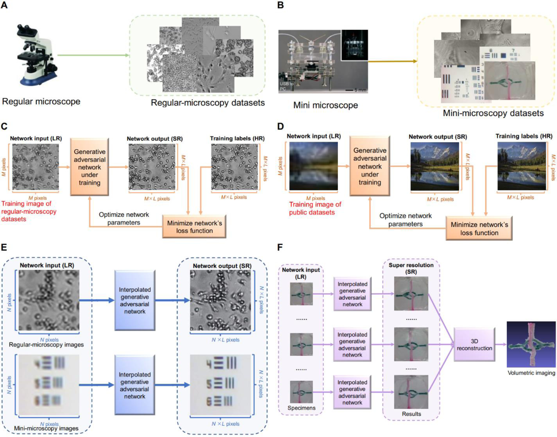
Schematic showing the design of our GAN-based SR algorithm in mini- and regular-microscopies for biomedical imaging. A) Regular-microscopy image acquisition in Section II.A. B) Mini-microscopy image acquisition in Section II.A. C) Training using cellular images from our regular-microscopy datasets in Section II.C.1). D) Training using natural images from public datasets in Section II.C.1). E) Testing the interpolated network using regular-microscopy and mini-microscopy images in Section II.C.2). F) Volumetric mini-microscopy imaging of the specimen based on SR in Section III.B. Note that LR, SR, and HR are the abbreviations of low LR, SR, and HR, respectively.
2.1. Sample preparation
The experimental benchmark datasets included mini-microscopic images and regular-microscopic images acquired with different objectives.
Regular-microscopy image acquisition.
Images of A549 human lung carcinoma cells at magnifications of ×2, ×4, ×10, ×20, and ×40, images of C2C12 mouse skeletal muscle cells at magnifications of ×4, ×10, ×20, and ×40, images of HepG2 human hepatocellular carcinoma cells at magnifications of ×4, ×10, ×20, and ×40, and images of human umbilical vein endothelial cells (HUVECs) at magnifications of ×2, ×4, ×10, ×20, and ×40 were obtained in-lab using a Zeiss Axio Observer D1 optical microscope. These regular-microscopy images were randomly divided into a training, validation, and testing dataset.
Mini-microscopy image acquisition.
We also used our lab-made low-cost (~$10) mini-microscope to observe the NIH/3T3 fibroblasts [25,26]. By varying the distance between the lens and the CMOS sensor using a spacer constructed from an Eppendorf tube, we could obtain a continuous gradient of magnifications. Using this approach, we were able to equip the mini-microscope with ×8, ×20, ×40, and ×60 magnifications at a lens-to-sensor distance of 5 mm (no spacer), 12 mm, 24 mm, and 48 mm, respectively. All the mini-microscopy images were from our previous publications [25,26] with permissions, and were all used as testing datasets in this paper.
2.2. Image pre-processing
Following general SR methods, all experiments were performed with a scaling factor of ×4 between LR and HR images. We collected the regular-microscopy images and mini-microscopy images as HR images. LR images were obtained by down-sampling HR images using the MATLAB Bicubic kernel function [17]. The spatial size of cropped HR patches was 128 × 128 pixels. One LR image and One HR image were paired. In Section III.A, regular-microscopy images were divided into training, validation, and testing datasets for training the network. Mini-microscopy images were utilized as the testing dataset.
2.3. GAN structure and training
SR methods based on GAN can encourage the network to favor solutions that appear more like natural images. One of the milestones towards visually pleasing results is the enhanced SRGAN (ESRGAN) [9], which borrows the idea from relativistic average GAN (RaGAN) to let the discriminator predict relative realness instead of the absolute value [28]. ESRGAN ran smoothly on images captured in a non-cellular environment for exceptional image quality and real-time responsiveness, yet, it is not specialized to cellular images and may fail to recover the cell-specific texture or patterns. To that end, we will introduce a novel ESRGAN(cell) to improve the baseline ESRGAN through an interpolation scheme. In sections that follow, we (i) introduce the backbone network for ESRGAN; (ii) develop a novel GAN network ESRGAN(cell); and (iii) combine the strengths of both through network interpolation.
2.3.1. Deep network backbone
Our deep neural network adopted ESRGAN serves as the basic network building block. To introduce biological cellular features into ESRGAN while retaining the ability to recover natural objects, a flexible and effective strategy, namely network parameter interpolation, was applied. The ESRGAN consisted of two sub-networks which were trained simultaneously, a generator G which enhances the input LR image, and a discriminator D which returns an adversarial loss to the resolution-enhanced image.
ESRGAN optimized the SR task by minimizing the sum of the generator loss LG and discriminator loss LD:
| (1) |
where θG is the generator parameter and θD denotes the discriminator parameter. The adversarial loss for generator LG is the combination of the original adversarial loss with the 1-norm loss L1 and the perceptual loss Lpercep:
| (2) |
where λ and η are coefficients to balance different loss terms.
To allow our generator to benefit from the gradients of the both generated and real data during adversarial training, the adversarial generator loss was applied, which was in a symmetrical form of the discriminator loss in Eq. 10:
| (3) |
where, Exr[⋅] represents the empirical expectation considering all real data xr in the mini-batch and Exf [⋅] denotes the empirical expectation considering all fake data xf = G(x) in the mini-batch, which is recovered by the generator G. As the original adversarial loss contains both the real image xr and the recovered image xf, our generator benefits from the gradients of both SR and real data in adversarial training.
The relativistic discriminator DRa of RaGAN in Eq. 3 in ESRGAN was defined as:
| (4) |
and
| (5) |
where S is the sigmoid function, C(x) is the non-transformed discriminator output. The used sigmoid function is defined as .
The previous GAN-based image-restoration methods have reported that using the GAN without the norm functions leads to object contour deformation [46]. Image-restoration algorithms using L1 norm or L2 norm are able to recover object contours [47]. This different result is attributed to the fact that L1 norm and L2 norm conduct pixel-wise operations between a generated image and a real image to constrain the contour of the object. Besides this, a GAN-based method restores information from the original image as a whole. This operation lakes constraint on the contour of the object. For this reason, a norm was adopted to train the generator in GAN-based applications. Moreover, as L1 norm is able to provide sparse resolutions, theoretically, image-restoration methods based on L1 norm has better potential to generate sharper images than L2 norm-based approaches.
Here we defined L1 to evaluate the 1-norm distance between recovered image xf and ground truth xr. The formulation is shown as:
| (6) |
where xf = G(x) is the recovered image, and xr is the ground truth. ‖ ‖1 is the function of the 1-norm distance.
To restore more accurate brightness and realistic textures, a perceptual loss Lpercep that evaluates a solution regarding perceptually relevant characteristics was employed [28]. The definition of perceptual loss was demonstrated as:
| (7) |
Here, φ is the coefficients to balance different loss terms. LCon is the content loss, which was obtained by calculating the Euclidean distance between the feature representations of a reconstructed image xf and the reference image xr:
| (8) |
where W and H describe the dimensions of the feature maps ϕ within the network, respectively.
The generative loss is:
| (9) |
where the standard GAN discriminator is the probability that the reconstructed image xf is a natural HR image. S is the sigmoid function, and C(xf) is the non-transformed discriminator output of the reconstructed image xf. The used sigmoid function is defined as .
The discriminator loss LD was formulated as:
| (10) |
Here, Exf [⋅] denotes the average of all fake data in the mini-batch. Exr [⋅] represents the average of all real data in the mini-batch. As reported in the literature [9], this discriminator loss facilitates learning sharper edges and more detailed textures.
2.3.2. Network training schedule
The training datasets of ESRGAN(cell) were cells images captured with a regular-microscope, and the operational process of image acquisition is elaborated in Section II.A. After retraining, ESRGAN(cell) attained updated parameters that were different from those of ESRGAN. To be familiar with both cellular and non-cellular images, we designed a network-interpolation method to combine merits of ESRGAN and ESRGAN(cell).
The training process was divided into two stages. ESRGAN served as the basic network building block. In the first stage, we used a pre-trained model of ESRGAN [9] that was trained on the natural images from the DIV2K dataset and the Flickr2K dataset [19–20]. ESRGAN tended to perform a SR operation on specimen images without cellular structures. In the second stage, we used the training dataset of our regular-microscopy images to obtain the model, namely ESRGAN(cell). The mini-batch size was set to 8. The learning rate was initialized as 1 × 10⁻⁴ and halved at [5 × 10³, 1 × 10⁴, 2 × 10⁴, 3 × 10⁴] iterations. We utilized the Adam optimization strategy with β1 = 0.9 and β2 = 0.9. The coefficients λ and η in Eq. 2, as well as φ in Eq. 7 were identical to the parameters used in ESRGAN [9]. As a result, ESRGAN(cell) managed to integrate cellular details into the image SR process. This framework was implemented by PytTorch framework version 1.1.0 and Python version 3.6.4 in the Microsoft Windows 10 Pro operating system [29–30]. The training was performed on a consumer-grade laptop (G5 15, Dell PC) equipped with a GeForce GTX 1060 with max-Q design graphic cards (NVDIA) and a Core i5–8300H CPU @ 2.30 GHz (Intel).
2.3.3. Network interpolation
Following the training schedule in Section II.C.1), we obtained two networks, namely ESRGAN and ESRGAN(cell). We interpolated all of the corresponding parameters of these two networks to derive an interpolated model , whose parameters were defined as:
| (11) |
where , and are the parameters of G G respectively, α ∈ [0,1] is the interpolation parameter.
When testing, the traditional ESRGAN loaded the parameters trained by natural images layer by layer. Unlike ESRGAN, ESRGAN* updated the original parameters of ESRGAN in testing by using Eq. 11 and then replaced the original parameters of ESRGAN with the updated parameter values layer-by-layer.
We reported an ablation study to evaluate the effect of the proposed network-interpolation strategy in Section III.C.
2.3.4. Implementation of biomedical volumetric imaging
Since HR images with fine details can improve the quality of 3D reconstruction, we conducted volumetric imaging experiments to further evaluate the performance of our method. Volumetric imaging was implemented with the VisualSFM software with CMVS/PMVS and the MeshLab software in the Microsoft Windows 10 Pro operating system [31–33]. The VisualSFM software generated sparse point clouds by utilizing the structure from motion (SFM) [34], including feature detection, feature matching, and bundle adjustment. For dense reconstruction, VisualSFM integrated the execution of Yasutaka Furukawa’s PMVS/CMVS tool chain [35]. The 3D model output by VisualSFM was imported into MeshLab for more useful and appealing 3D visualization. The detailed results of volumetric imaging are illustrated in Section III.B.
3. Results and discussions
In this paper, we quantified the accuracy of estimates with two metrics, namely the peak signal-to-noise ratio (PSNR) index and structural similarity (SSIM) index [36,37].
PSNR is defined as:
| (12) |
where is the maximum possible pixel value of the image I. MSE is referred to as the mean squared error [38], which was obtained by:
| (13) |
where I is a noise-free m × n monochrome image and K represents its noisy approximation.
SSIM is defined as:
| (14) |
where x is the LR input, y is the HR image used as ground truth, μx, μy are the averages of x, y; σx, σy are the standard deviations of x, y; σx,y is the covariance of x and y; and c1, c2, c3 are the variables used to stabilize the division with a small denominator. Generally, we set c3 = c2/2, and SSIM could be re-written as:
| (15) |
Higher PSNR and SSIM values are preferred as this indicates the reconstruction was of superior quality. An SSIM value of 1.0 indicates identical images.
3.1. Qualitative and quantitative comparisons
We compared our final models on our biomedical benchmark datasets with state-of-the-art deep learning methods, including EDSR [39], FALSR [40], DPSR [41], SRGAN [28], and ESRGAN [9]. The conventional Bicubic method was also listed in comparisons [17]. Acquisition of the experimental dataset was elaborated in Section II.A. To promote objective comparison, all competitive deep learning methods were retrained using the same databases as the ESRGAN(cell) was, besides their original databases. In this paper, these competitive deep-learning methods followed the training process operations, which are illustrated in their respective references. In each case, initial training parameter settings were consistent with those in the original references.
Comparisons on regular-microscopy images.
The 112 regular-microscopy images, as HR images, were split into a training dataset consisting of 53 images, a validation dataset consisting of 20 images, and a testing dataset consisting of 39 images. All images were 2048 × 2048 pixels. To enrich our training and validation datasets, we cropped sub-images from images in the training and validation datasets by using a sliding window with a step length of 186 pixel. In this way, the final training and validation datasets were extended to 6,413 and 2,420 images, respectively. All HR images were 360 × 360 pixels. These HR images were down-sampled to 90 × 90 pixels by using Bicubic [17]. Fig. 2 depicts PSNR and SSIM plots of different SR methods over all regular-microscopy images. These PSNR and SSIM plots demonstrate that the algorithm ESRGAN* proposed here exhibited superior performance relative to the other seven state-of-the-art methods. PSNR was evaluated on the luminance channel in the YCbCr color space and SSIM measured the structural accuracy of the reconstructed image.
Fig. 2.

PSNR and SSIM plots of different SR methods over all regular-microscopy images, including A549 at magnifications of 2×, 4×, and 10×, C2C12 at magnification of 4× and 10×, HepG2 at magnification of 10×, as well as HUVECs at magnification of 10× at both high densities and low densities. The methods evaluated include Bicubic [17], EDSR [39], FALSR [40], DPSR [41], SRGAN [28], ESRGAN [9], and ESRGAN*. Quantitative estimates were made based on PSNR and SSIM [36,37]. The corresponding PSNR and SSIM are displayed in the format of (PSNR /SSIM) below each sub-image. PSNR represents the errors of the corresponding pixels between two images. SSIM measures image similarity in terms of brightness, contrast, and structure. PSNR and SSIM are defined in Eq. 12 and Eq. 15, respectively. A higher PSNR and a higher SSIM generally indicate that the reconstruction is of higher quality. ESRGAN* performed favorably against ESRGAN.
Table 1 (top part) reports quantitative results, including average PSNR and average SSIM of the seven different SR methods over all regular-microscopy images shown in Fig. 2. Qualitative comparisons of different SR methods in the regular-microscopy images are illustrated in Fig. 3, which indicated that the ESRGAN* outperformed previous approaches such as ESRGAN and SRGAN in both sharpness and details. For example, ESRGAN* generated clearer and better visual perceptual quality in A549 at magnifications of 2× and 4× than the PSNR-oriented approaches, which tended to generate blurry outputs. ESRGAN* was capable of reproducing more detailed structures in C2C12 at magnifications of 4× than the other GAN-based methods, such as ESRGAN and SRGAN, whose textures were unnatural and included unpleasant noise. Since our method ESRGAN* interpolated two sets of network parameters of natural and biomedical images, respectively, it provided a new way to incorporate two different training results, while simultaneously solving the problem that the number of images in the two training datasets were unbalanced. Compared with ESRGAN, ESRGAN* were artifact-free and output more pleasing results.
Table 1.
Average PSNR and average SSIM of the seven different SR methods over all regular-microscopy and mini-microscopy images showing in Fig. 3.
| Regular-microscopy Images | |||||||
|---|---|---|---|---|---|---|---|
| Metrics╲Methods | Bicubic [17] | EDSR [39] | FALSR [40] | DPSZ [41] | SRGAN [28] | ESRGAN [9] | ESRGAN* |
| Average PSNR | 28.15 | 30.69 | 29.90 | 28.48 | 27.38 | 26.39 | 31.03 |
| Average SSIM | 0.80 | 0.86 | 0.86 | 0.81 | 0.77 | 0.73 | 0.88 |
| Mini-microscopy images | |||||||
| Metrics╲Methods | Bicubic [17] | EDSR [39] | FALSR [40] | DPSZ [41] | SRGAN [28] | ESRGAN [9] | ESRGAN* |
| Average PSNR | 33.64 | 35.37 | 33.99 | 32.98 | 29.20 | 33.83 | 35.85 |
| Average SSIM | 0.81 | 0.84 | 0.84 | 0.80 | 0.81 | 0.82 | 0.85 |
This experiment followed the setup and used the same metrics as comparisons on regular-microscopy images shown in Fig. 2. A higher PSNR and a higher SSIM generally indicate that the reconstruction is of higher quality. Our ESRGAN* outperformed alternative state-of-the-art approaches. The first, second, and third best are identified with red, blue, and green, respectively.
Fig. 3.

Comparisons of different SR methods in the regular-microscopy images, including A549 at magnifications of 2×, 4×, and 10×, C2C12 at magnification of 4× and 10×, HepG2 at magnification of 10×, as well as HUVECs at magnification of 10× at both high and low densities. The evaluated methods were Bicubic, EDSR, FALSR, DPSR, SRGAN, ESRGAN, and ESRGAN*. This experiment followed the setup and used the same metrics as comparisons on regular-microscopy images shown in Fig. 2. Our ESRGAN* performed favorably against alternative state-of-the-art approaches.
This experiment followed the setup and used the same metrics as comparisons on regular-microscopy images shown in Fig. 2.
Comparisons on mini-microscopy images.
For this comparison, we directly used the trained network in the above section of Comparisons on regular-microscopy images. A total of seven mini-microscopy images were utilized as HR images for the testing dataset. All HR images were 640 × 480 pixels. These HR images were down-sampled to 160 × 120 pixels by using Bicubic. Fig. 4 displays PSNR and SSIM plots of different SR methods over all mini-microscopy images. The evaluated methods were Bicubic, EDSR, FALSR, DPSR, SRGAN, ESRGAN, and ESRGAN*. ESRGAN* performed favorably, relative to state-of-the-art approaches. Compared with ESRGAN, ESRGAN* utilized the network-interpolation strategy to balance the effects of the network trained based on natural images and the network trained based on cellular images. ESRGAN produced the over-sharp contours of the restored images. The previous GAN-based approach, e.g., SRGAN, lacked the prediction of relative realness and only measured whether one image was real or fake. Therefore, SRGAN introduced distracting and potentially misleading artifacts into the restored images. Moreover, the other methods without the perceptual loss, either added undesired textures (EDSR, FALSR) or failed to generate enough details (Bicubic, DPSR).
Fig. 4.

PSNR and SSIM plots of different SR methods over all mini-microscopy images, for NIH/3T3 fibroblasts at magnifications of 8×, 20×, 40×, and 60×, with Mini1, Mini2, and Specimen (Mini1, Mini2, and Specimen are mini-microscopy images of the resolution target shown in Fig. 5). The methods evaluated include Bicubic, EDSR, FALSR, DPSR, SRGAN, ESRGAN, and ESRGAN*. This experiment followed the setup and used the same metrics as comparisons on regular-microscopy images shown in Fig. 2. Our ESRGAN* performed favorably against alternative state-of-the-art approaches.
Table 1 (bottom panel) summarizes quantitative results, including average PSNR and average SSIM of seven different SR methods over all mini-microscopy images in Fig. 4. Qualitative comparisons of different SR methods in the mini-microscopy images are illustrated in Fig. 5. As depicted in Fig. 5, ESRGAN* achieved consistently better visual qualities, consisting of more realistic and clear structures than the other methods. This could be attributed to the fact that we used two different sets of training data comprised of biomedical and natural images, respectively. Based on this fact, we trained the relativistic GAN to encourage the discriminator measure the probability that the synthetic data was more realistic than the real data, rather than computing the absolute error between the synthetic data and the real data. Therefore, ESRGAN* can provide stronger supervision for texture recovery and higher reconstruction accuracy.
Fig. 5.

Comparisons of different SR methods in the mini-microscopy images, for NIH/3T3 fibroblasts at magnifications of 8×, 20×, 40×, and 60×, Mini1, Mini2, and Specimen (Mini1, Mini2, and Specimen are mini-microscopy images of the resolution targets). The methods evaluated include Bicubic, EDSR, FALSR, DPSR, SRGAN, ESRGAN, and ESRGAN*. This experiment followed the setup and used the same metrics as comparisons on regular-microscopy images shown in Fig. 2. ESRGAN* performed favorably relative to alternative state-of-the-art approaches.
Discussion.
ESRGAN* was superior to Bicubic and other competitive deep-learning SR methods. Bicubic executes the interpolate operation in the neighborhood. This method only considers the local pixel values and is short of objective features. Therefore, Bicubic fails to restore details of objects and leads to image degradation. The SR-enhanced images by DPSR appear over-smoothed globally and over-sharpened locally. This is caused by the introduced arbitrary blur kernel, which focuses on deblurring when super-resolving [41]. Compared with ESRGAN*, EDSR and FALSR are also deep learning-based super resolvers. However, EDSR and FALSR restore SR images without enough high-frequency information, due to lack of the measurement of perceptual vision. ESRGAN* utilizes a RaGAN [28] rather than a standard GAN [9] in SRGAN [28], and this encourages the discriminator to predict relative realness in place of the image errors which are calculated by the Manhattan Distance between the real image and the fake image. In this way, ESRGAN* provides more natural and visually pleasant restored images, while ESRGAN-enhanced images contained nonexistent “phantom” details, which correspond to unintended artifacts that could lead a human viewer to make misinterpret details. Depending on the context, such human error could range from inconvenience to potential harmful decisions. ESRGAN combining original training databases comprised of natural images, and the cellular training databases in Section II.A. However, this makes ESRGAN biased towards large databases, since this training database setting loses sight of different amounts in original training databases and biomedical training databases. In contrast, ESRGAN* employs the network parameter interpolation to directly combine the network parameters. Hence, ESRGAN* is capable of balancing the effects of databases of different sizes.
3.2. Volumetric imaging based on SR
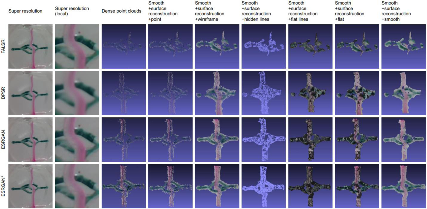
Volumetric imaging is affected by the input image quality, which usually benefits from HR images. We demonstrate that our ESRGAN* model can also benefit volumetric imaging. Fig. 6 shows mini-microscopic volumetric imaging using VisualSFM [31] and MeshLab [33]. The LR images were multiple 2D images captured by the mini-microscope from different view angles of a biomedical specimen [25,27], which was a transparent elastomeric object with bioprinted color patterns on the two opposing surfaces. These LR images were input into our model to generate HR images. The results showed that our ESRGAN* could recover fine details of the original images that leads to improved volumetric imaging. This is mainly due to the fact that ESRGAN* used the relativistic average GAN (RaGAN) that allows the discriminator to predict relative realness. However, other algorithms, such as FALSR and DPSR, did not use GAN to achieve the real structural information. Moreover, DPSR over smoothen the details during restoration, and then lost substantial texture information. FALSR simplified the SR model by utilizing the elastic search, which combined the cell-level micro and intercell macro search spaces. This search method boosted running speed during mapping, but some detailed structural information was lost. Fig. 7 shows another biomedical volumetric imaging with bioprinted microchannels. We also utilized VisualSFM to produce dense point clouds, and then conducted surface reconstruction as well as texturing on MeshLab. As only the super-resolved images based on ESRGAN* could output 3D structure, ESRGAN* was proven superior to other experimental methods. Results of imaging of 3D cellular structure together with comparisons with other methods are given in Appendix.
Fig. 6.
Biomedical volumetric imaging using VisualSFM and MeshLab. Seven different SR approaches were utilized in total to transform LR images of the specimen into SR ones. VisualSFM uses the SR images to produce corresponding sparse and dense point clouds. MeshLab runs smooth and surface reconstruction operations on the dense point clouds. We show six types of modeling results, including point, wireframe, hidden lines, flat lines, flat, and smooth. Only FALSR, DPSR, ESRGAN, and ESRGAN* methods could successfully output 3D reconstruction models.
Fig. 7.

Biomedical volumetric imaging using VisualSFM and MeshLab. Among the seven different SR approaches, only ESRGAN* was successful to output 3D reconstruction model. VisualSFM uses the SR images to produce corresponding sparse and dense point clouds. MeshLab runs the screened-Poisson-based surface reconstruction operation and the texturing operation on the dense point clouds.
3.3. Ablation study
We subsequently compared the effectiveness of the network-interpolation strategy in Eq. 11 to balance the results of an ESRGAN model and an ESRGAN(cell) model. We applied simple linear interpolation on the scheme and compared their differences. The interpolation parameter α was chosen from the interval (0,1) with an interval of 0.05.
The overall visual comparison was illustrated in Fig. 8, in order to explore which value of α generated the best results. The ablation study was adopted to show the results which were generated by different values of α. The testing dataset utilized all images of the regular-microscopy dataset in Section II.A, including A549 at magnifications of 2×, 4× and 10×, C2C12 at magnifications of 4× and 10×, HepG2 at magnification of 10×, as well as HUVECs at magnification of 10× with high density and low density as testing dataset. Fig. 8 shows two plots based of two different the PSNR and SSIM metrics. Each plot consists of a single line, the average PSNR/SSIM over all testing dataset. The yellow sign indicates the maxima of all PSNR values or SSIM values. As depicted in Fig. 8, when α in Eq. 11 was set to 0.25, ESRGAN* attained the best results in terms of PSNR and SSIM. Furthermore, this parameter setting also revealed that ESRGAN* achieved the best balance between restoration of natural and biomedical images. These two plots demonstrate that larger or smaller values of α degrade the performance of the ESRGAN* in terms of pixel-wide precision for PSNR and structure precision relative to SSIM.
Fig. 8.

PSNR and SSIM plots of ablation study of ESRGAN* in Eq. 10 over all regular-microscopy images, including A549 at magnifications of 2×, 4× and 10×, C2C12 at magnifications of 4× and 10×, HepG2 at magnification of 10×, as well as HUVECs at magnification of 10× with high and low density. This experiment followed the setup and used the same metrics as comparisons on regular-microscopy images shown in Fig. 2. The yellow sign indicates the maxima of the all PSNR values or SSIM values. Α ∈ [0,1] is the interpolation parameter in Eq. 11. The sampling interval of α is 0.05. Setting α to 0.25 enabled ESRGAN* to attain the best results for both PSNR and SSIM.
4. Conclusions
This paper presented a novel SR algorithm ESRGAN*, which combined merits of ESRGAN and ESRGAN(cell). ESRGAN possessed the GAN-based framework comprising a generative model, which improved the input LR image and a discriminative model that reported an adversarial loss to the improved image. The adversarial loss involved a novel perceptual loss that enabled the discriminator to predict relative realness, instead of the absolute value. In this manner, ESRGAN achieved consistent visual quality with realistic and natural texture recovery. The training of ESRGAN was based on the DIV2K and Flickr2K datasets, providing it with the ability of adapt to non-cellular images. The ESRGAN(cell) possessed the same network structure as ESRGAN, but parameter setting differed from ESRGAN. Given that ESRGAN served as the baseline framework, ESRGAN(cell) retrained ESRGAN by utilizing our specific regular-microscopy training datasets, so as to possess the ability to restore cellular details. ESRGAN and ESRGAN(cell) were further integrated by implementing network interpolation to generate a new deep learning network named ESRGAN*. As a result, ESRGAN* inherited the strengths of ESRGAN and ESRGAN(cell) such as realistic and natural texture recovery both for images with cells as well as natural images. ESRGAN* outperformed the state-of-the-art methods on both regular-microscopy and mini-microscopy datasets in terms of qualitative and quantitative evaluation methods. Moreover, the volumetric imaging based on ESRGAN* was also superior to the volumetric imaging results based on other SR approaches. The integrality and exactness of stereo imaging of ESRGAN* demonstrated its superiority for SR applications in multiple application domains.
Supplementary Material
Highlights.
A deep learning-enabled super-resolution (SR) imaging method
The method applicable to both regular and mini-microscopy
Network interpolation strategy to incorporate biological cellular features into SR
Hardware for SR imaging at an extremely low cost (<$10) in mini-microscopy
Improve volumetric SR imaging for spatial analyses in mini-microscopy
6. Acknowledgements
This work was supported in part by the University of Massachusetts Dartmouth College of Engineering faculty start-up funding, the Brigham Research Institute, and the National Institutes of Health (R03EB027984, R01EB028143). We thank Haziq Jeelani and Shabir Hassan for their help in useful discussions during early stages of the project.
Author Biographies
Manna Dai received her Ph.D. degree in Computer Science from Faculty of Engineering and Information Technology, University of Technology Sydney, Australia. She was affiliated with Data61, Commonwealth Scientific and Industrial Research Organization, Australia. She conducted her postdoctoral research in the Division of Engineering in Medicine, Department of Medicine, Brigham and Women’s Hospital, Harvard Medical School, USA. Her research interests include target tracking, machine learning, deep learning, computer vision, and image-processing.
Gao Xiao received his B.S. and Ph.D. degrees from Sichuan University, China in 2008 and 2014, respectively. Then, he worked as an Assistant Professor at College of Environment and Resources, Fuzhou University, Fuzhou, China. Since 2017, he has been working as a Senior Postdoctoral Researcher in John A. Paulson School of Engineering and Applied Sciences, Harvard University, USA. He is also affiliated with Wyss Institute for Biologically Inspired Engineering, Harvard University, and Brigham and Women’s Hospital, Harvard Medical School, USA. His research interests include nanotechnology, bio-imaging science, intelligent systems for molecular biology, nanomedicine and medical image processing.
Lance Fiondella received his Ph.D. degree in Computer Science & Engineering from the University of Connecticut in 2012. He is an Associate Professor of Electrical and Computer Engineering at the University of Massachusetts Dartmouth. His peer-reviewed conference papers have been the recipient of 12 awards. Dr. Fiondella served as the vice-chair of IEEE Standard 1633: Recommended Practice on Software Reliability 2013–2015 and a 3-year term as a Member of the Administrative Committee of the IEEE Reliability Society 2015–2017. He presently serves as a technical committee chair of the Annual IEEE Symposium on Technologies for Homeland Security.
Ming Shao received his Ph.D. degree in Computer Engineering from Northeastern University, 2016. He is a tenure-track Assistant Professor affiliated with College of Engineering at the University of Massachusetts Dartmouth since 2016 Fall. His current research interests include predictive modeling, adversarial machine learning, robust visual representation learning, and health informatics. He was the recipient of the Presidential Fellowship of State University of New York at Buffalo from 2010 to 2012, and the best paper award winner of IEEE ICDM 2011 Workshop on Large Scale Visual Analytics, and best paper award candidate of ICME 2014. He is the Associate Editor of SPIE Journal of Electronic Imaging, and IEEE Computational Intelligence Magazine. He is a member of IEEE.
Dr. Zhang received a B.Eng. in Biomedical Engineering from Southeast University, China (2008), a M.S. in Biomedical Engineering from Washington University in St. Louis (2011), and a Ph.D. in Biomedical Engineering at Georgia Institute of Technology/Emory University (2013). Dr. Zhang is currently an Assistant Professor at Harvard Medical School and Associate Bioengineer at Brigham and Women’s Hospital. Dr. Zhang’s research is focused on innovating medical engineering technologies, including bioprinting, organs-on-chips, microfluidics, and bioanalysis, to recreate functional tissues and their biomimetic models towards applications in precision medicine.
Footnotes
Publisher's Disclaimer: This is a PDF file of an unedited manuscript that has been accepted for publication. As a service to our customers we are providing this early version of the manuscript. The manuscript will undergo copyediting, typesetting, and review of the resulting proof before it is published in its final form. Please note that during the production process errors may be discovered which could affect the content, and all legal disclaimers that apply to the journal pertain.
5. Conflicts of interest
There are no conflicts to declare.
Declaration of interests
The authors declare that they have no known competing financial interests or personal relationships that could have appeared to influence the work reported in this paper.
References
- [1].Lecun GOY, Bengio Y, and Hinton G, Deep learning, Nature, 521 (7553) (2015) 436–444. [DOI] [PubMed] [Google Scholar]
- [2].Pouyanfar S, Sadiq S, Yan Y, Tian H, Tao Y, Reyes MP, Shyu M-L, Chen S-C, and Iyengar SS, A survey on deep learning: algorithms, techniques, and applications, ACM Computing Surveys, 51 (5) (2018) 1–36. [Google Scholar]
- [3].Constantin MD, Elena M, Peter S, Nguyen PH, Madeleine G, and Antonio L, Scalable training of artificial neural networks with adaptive sparse connectivity inspired by network science, Nature Communications, 9 (1) (2018) 1–12. [DOI] [PMC free article] [PubMed] [Google Scholar]
- [4].Rivenson Y, Göröcs Z, Günaydin H, Zhang Y, Wang H, and Ozcan A, Deep learning microscopy, Optica, 4 (11) (2017) 1437–1443. [Google Scholar]
- [5].Burrello A, Schindler K, Benini L, and Rahimi A, Hyperdimensional computing with local binary patterns: one-shot learning of seizure onset and identification of Iictogenic brain regions using short-time iEEG recordings, IEEE Transactions on Biomedical Engineering, 67 (2) (2020) 601–613. [DOI] [PubMed] [Google Scholar]
- [6].González G, Ash SY, Vegas Sanchez-Ferrero G, Onieva Onieva J, Rahaghi FN, Ross JC, Díaz A, Raúl SJE, and Washko GR, Disease staging and prognosis in smokers using deep learning in chest computed tomography, American Journal of Respiratory & Critical Care Medicine, 197 (2) (2018) 193–203. [DOI] [PMC free article] [PubMed] [Google Scholar]
- [7].Kermany DS, Goldbaum M, Cai W, Valentim CCS, Liang H, Baxter SL, McKeown A, Yang G, Wu X, Yan F, Dong J, Prasadha MK, Pei J, Ting MYL, Zhu J, Li C, Hewett S, Dong J, Ziyar I, Shi A, Zhang R, Zheng L, Hou R, Shi W, Fu X, Duan Y, Huu VAN, Wen C, Zhang ED, Zhang CL, Li O, Wang X, Singer MA, Sun X, Xu J, Tafreshi A, Lewis MA, Xia H, and Zhang K, Identifying medical diagnoses and treatable diseases by image-based deep learning, Cell, 172 (5) (2018) 1122–1131. [DOI] [PubMed] [Google Scholar]
- [8].Wang G, Li W, Zuluaga MA, Pratt R, Patel PA, Aertsen M, Doel T, David AL, Deprest J, and Ourselin S, Interactive medical image segmentation using deep learning with image-specific fine-tuning, IEEE Transactions on Medical Imaging, 37 (7) (2018) 1562–1573. [DOI] [PMC free article] [PubMed] [Google Scholar]
- [9].Wang X, Yu K, Wu S, Gu J, and Loy CC, ESRGAN: enhanced super-resolution generative adversarial networks, in Proc. European Conference on Computer Vision (ECCV), (2018). [Google Scholar]
- [10].Junjun Jiang, Yi Yu, Zheng Wang, Suhua Tang, Ruimin, and Hu, Ensemble super-resolution with a reference dataset, IEEE Transactions on Cybernetics, (2019). [DOI] [PubMed] [Google Scholar]
- [11].Chen C, Xiong Z, Tian X, Zha Z-J, and Wu F, Camera lens super-resolution, in Proc. IEEE Conference on Computer Vision and Pattern Recognition, (2019) 1652–1660. [Google Scholar]
- [12].Isoa P, Zhu J-Y, Zhou T, and Efros A, Image-to-image translation with conditional adversarial networks, in Proc. IEEE Conference on Computer Vision and Pattern Recognition, (2017) 1125–1134. [Google Scholar]
- [13].Yeh RA, Chen C, Lim TY, Schwing AG, and Do MN, Semantic image inpainting with deep generative models, in Proc. IEEE Conference on Computer Vision and Pattern Recognition, (2017) 5485–5493. [Google Scholar]
- [14].Ma J, Xu H, Jiang J, Mei X, Zhang X, DDcGAN: A dual-discriminator conditional generative adversarial network for multi-resolution image fusion, IEEE Transactions on Image Processing, 29 (2020) 4980–4995. [DOI] [PubMed] [Google Scholar]
- [15].Zhang H, Xu T, Li H, Zhang S, Wang X, Huang X, and Metaxas D, StackGAN: text to photo-realistic image synthesis with stacked generative adversarial networks, in Proc. IEEE International Conference on Computer Vision, (2017) 5907–5915. [Google Scholar]
- [16].Chen R, Qu Y, Zeng K, Guo J, and Xie Y, Persistent memory residual network for single image super resolution, in Proc. IEEE Conference on Computer Vision and Pattern Recognition Workshops (CVPRW), (2018) 809–816. [Google Scholar]
- [17].Nah S, Baik S, Hong S, Moon G, Son S, Timofte R, and Lee KM, NTIRE 2019 challenge on video deblurring and super-resolution: dataset and study, in Proc. IEEE Conference on Computer Vision and Pattern Recognition Workshops (CVPRW), (2019). [Google Scholar]
- [18].Song P, Deng X, Mota JFC, Deligiannis N, and Rodrigues MRD, Multimodal image super-resolution via joint sparse representations induced by coupled dictionaries, IEEE Transactions on Computational Imaging, 6 (2019) 57–72. [Google Scholar]
- [19].Agustsson E, and Timofte R, NTIRE 2017 challenge on single image super-resolution: dataset and study, in Proc. IEEE Conference on Computer Vision and Pattern Recognition Workshops (CVPRW), (2017) 126–135. [Google Scholar]
- [20].Timofte R, Agustsson E, Gool LV, Yang MH, and Guo Q, NTIRE 2017 challenge on single image super-resolution: methods and results, in Proc. IEEE Conference on Computer Vision and Pattern Recognition Workshops (CVPRW), (2017) 114–125. [Google Scholar]
- [21].Lu R, Liang Y, Meng G, Zhou P, and Ji N, Rapid mesoscale volumetric imaging of neural activity with synaptic resolution, Nature Methods, 17 (3) (2020) 291–294. [DOI] [PMC free article] [PubMed] [Google Scholar]
- [22].Truong TV, Holland DB, Madaan S, Andreev A, and Fraser SE, High-contrast, synchronous volumetric imaging with selective volume illumination microscopy, Communications Biology, 3 (1) (2020) 1–8. [DOI] [PMC free article] [PubMed] [Google Scholar]
- [23].Zhou T, Thung KH, Liu M, and Shen D, Brain-wide genome-wide association study for alzheimer’s disease via joint projection learning and sparse regression model, IEEE Transactions on Biomedical Engineering, 66 (1) (2018) 165–175. [DOI] [PMC free article] [PubMed] [Google Scholar]
- [24].Hyde D, Peters JM, and Warfield S, Multi-resolution graph based volumetric cortical basis functions from local anatomic features, IEEE Transactions on Biomedical Engineering, 66 (12) (2019) 3381–3392. [DOI] [PMC free article] [PubMed] [Google Scholar]
- [25].Zhang YS, Ribas J, Nadhman A, Aleman J, Selimovi Š, Lesher-Perez SC, Wang T, Manoharan V, Shin SR, Damilano A, Annabi N, Dokmeci MR, Takayama S, and Khademhosseini A, A cost-effective fluorescence mini-microscope for biomedical applications, Lab on a Chip, 15 (18) (2015) 3661–3669. [DOI] [PMC free article] [PubMed] [Google Scholar]
- [26].Zhang YS, Chang JB, Alvarez MM, Trujillo-De Santiago G, Aleman J, Batzaya B, Krishnadoss V, Ramanujam AA, Kazemzadeh-Narbat M, Chen F, Tillberg PW, Dokmeci MR, Boyden ES, and Khademhosseini A, Hybrid microscopy: enabling inexpensive high-performance imaging through combined physical and optical magnifications, Scientific Reports, 6 (2016) 22691. [DOI] [PMC free article] [PubMed] [Google Scholar]
- [27].Polat A, Hassan S, Yildirim I, Oliver LE, Mostafaei M, Kumar S, Maharjan S, Bourguet L, Cao X, Ying G, Hesar ME, and Zhang YS, A miniaturized optical tomography platform for volumetric imaging of engineered living systems, Lab on a Chip, 19, (4) (2019) 550–561. [DOI] [PMC free article] [PubMed] [Google Scholar]
- [28].Ledig C, Theis L, Huszar F, Caballero J, and Shi W, Photo-realistic single image super-resolution using a generative adversarial network, in Proc. IEEE Conference on Computer Vision and Pattern Recognition, (2017) 4681–4690. [Google Scholar]
- [29].Chen KM, Cofer EM, Zhou J, and Troyanskaya OG, Selene: a PyTorch-based deep learning library for sequence data, Nature Methods, 16 (4) (2019) 315–318. [DOI] [PMC free article] [PubMed] [Google Scholar]
- [30].Koch S, Schneider T, Williams F, and Panozzo D, Geometric computing with python, ACM SIGGRAPH 2019 Courses, (2019) 1–45.
- [31].Santagati C, Inzerillo L, and Paola FD, Image-based modeling techniques for architectural heritage 3D digitalization: limits and potentialities, Isprs International Archives of the Photogrammetry Remote Sensing & Spatial Information Sciences, 5 (2013) 555–560. [Google Scholar]
- [32].Matzen K, and Snavely N, Scene chronology, in Proc. European Conference on Computer Vision, (2014) 615–630. [Google Scholar]
- [33].Cignoni P, Callieri M, Corsini M, Dellepiane M, Ganovelli F, and Ranzuglia G, MeshLab: an open-source mesh processing tool, Eurographics Association, 2008 (2008) 129–136. [Google Scholar]
- [34].Kumar S, Jumping manifolds: geometry aware dense non-rigid structure from motion, in Proc. IEEE Conference on Computer Vision and Pattern Recognition, (2019) 5346–5355. [Google Scholar]
- [35].Qi S, Adams R, Curless B, Furukawa Y, and Seitz SM, The visual turing test for scene reconstruction, in Proc. 2013 International Conference on 3D Vision-3DV, (2013) 25–32. [Google Scholar]
- [36].Haris M, Shakhnarovich G, and Ukita N, Deep back-projection networks for super-resolution, in Proc. IEEE Conference on Computer Vision and Pattern Recognition, (2018) 1664–1673. [Google Scholar]
- [37].Gao S, and Zhuang X, Multi-scale deep neural networks for real image super-resolution, in Proc. IEEE Conference on Computer Vision and Pattern Recognition Workshops, (2019). [Google Scholar]
- [38].Bulat A, and Tzimiropoulos G, Super-FAN: integrated facial landmark localization and super-resolution of real-world low resolution faces in arbitrary poses with GANs, in Proc. IEEE Conference on Computer Vision and Pattern Recognition, (2018) 109–117. [Google Scholar]
- [39].Lim B, Son S, Kim H, Nah S, and Lee KM, Enhanced deep residual networks for single image super-resolution, in Proc. IEEE Conference on Computer Vision and Pattern Recognition Workshops, (2017) 136–144. [Google Scholar]
- [40].Chu X, Zhang B, Ma H, Xu R, Li J and Li Q, Fast, accurate and lightweight super-resolution with neural architecture search, (2019) arXiv preprint, arXiv:1901.07261.
- [41].Zhang K, Zuo W, and Zhang L, Deep plug-and-play super-resolution for arbitrary blur kernels, in Proc. IEEE Conference on Computer Vision and Pattern Recognition, (2019) 1671–1681. [Google Scholar]
- [42].Haan KD, Rivenson Y, Wu Y, and Ozcan A, Deep-learning-based image reconstruction and enhancement in optical microscopy, Proceedings of the IEEE, 108 (1) (2020) 30–50. [Google Scholar]
- [43].Wang H, Rivenson Y,Jin Y,Wei Z,Gao R,Günaydn H,Bentolila LA,Kural C,and Ozcan A, Deep learning enables cross-modality super-resolution in fluorescence microscopy, Nature Methods, 16 (2019) 103–110. [DOI] [PMC free article] [PubMed] [Google Scholar]
- [44].Rivenson Y, Zhang Y, Günaydin H, Teng D, and Ozcan A, Phase recovery and holographic image reconstruction using deep learning in neural networks, Light: Science & Applications, 7 (2018) 17141. [DOI] [PMC free article] [PubMed] [Google Scholar]
- [45].Sinha A, Lee J, Li S, and Barbastathis G, Lensless computational imaging through deep learning, Optica, 4 (9) (2017) 1117–1125. [Google Scholar]
- [46].Radford A, Metz L, and Chintala S, Unsupervised representation learning with deep convolutional generative adversarial networks, arXiv preprint arXiv:1511.06434, 2015-
- [47].Eslahi N, Aghagolzadeh A, Compressive sensing image restoration using adaptive curvelet thresholding and nonlocal sparse regularization, IEEE Transactions on Image Processing, 25(7) (2016) 3126–3140. [DOI] [PubMed] [Google Scholar]
Associated Data
This section collects any data citations, data availability statements, or supplementary materials included in this article.