Segmentation and Quantitative Analysis of Individual Cells in Developmental Tissues

Abstract

Image analysis is vital for extracting quantitative information from biological images and is used extensively, including investigations in developmental biology. The technique commences with the segmentation (delineation) of objects of interest from 2D images or 3D image stacks and is usually followed by the measurement and classification of the segmented objects. This chapter focuses on the segmentation task and here we explain the use of ImageJ, MIPAV (Medical Image Processing, Analysis, and Visualization), and VisSeg, three freely available software packages for this purpose. ImageJ and MIPAV are extremely versatile and can be used in diverse applications. VisSeg is a specialized tool for performing highly accurate and reliable 2D and 3D segmentation of objects such as cells and cell nuclei in images and stacks.

1. Introduction

Quantitative analysis of images is fast becoming an integral part of biological research, because such an approach extracts considerably more and accurate information from the sample. Usually the information serves as input for hypothesis testing complex biological processes by mathematical modeling, leading to improved understanding of the mechanisms and in some cases to subsequently improved diagnosis and treatment of major human diseases. However, most microscope images of biological samples are still analyzed manually, by subjective visual inspection.

Image Segmentation.

In general, quantitative analysis of images commences with segmentation (delineation) of the objects of interest, such as cells or cell nuclei. Segmentation can be performed either on 2D images or 3D image stacks and during the past 20 years, many algorithms have been developed to perform this task. Introductory information about segmentation and other aspects of image analysis is readily available in many textbooks [1–3] and Web sites [4].

Sample Preparation and Image Acquisition.

A prerequisite for obtaining quantitative 3D measurements from a sample is that the labeled sample is transparent. This is so that when imaging at a particular depth through the sample, the part of the sample in front of the depth does not obscure the image. Using flourescent labels ensure that this is the case, as well as bestowing two additional advantages: (1) Fluorescent labeling is quantitative because the intensity of the fluorescent signal is proportional to the concentration of the labeled molecules, (2) Multiple molecular species can be simultaneously imaged by employing fluorescent labels with different spectral properties. Thus, by using fluorescent labeling, one can visualize objects of interest in the biological samples, such as individual cells, subcellular organelles, and specific proteins of interest. Furthermore, fluorescent protein genetic constructs and certain fluorescent labels can be applied to living samples, thus enabling the extraction of structural, temporal, and spatial information about them.

Fluorescence microscopy advanced significantly in the 1980s with the advent of confocal microscopy, allowing direct acquisition of in focus 3D images from thick samples, and a decade later by the introduction of multi-photon microscopy enabling deeper penetration into living tissue.

For accurate quantification, particularly for 3D images, it is extremely important to prepare the samples with great care so as to avoid artifacts during imaging. In terms of image acquisition the objective lens is probably the most important component of the microscope since it determines the quality of images in terms of spatial resolution and sensitivity. It is best to use high numerical aperture (NA) oil immersion lenses for depths up to 50 μm and a water immersion lens for greater depths. Also, in order to capture as much spatial detail as possible from the sample it is necessary to use a voxel (Volume Picture Element: smallest distinguishable box in a 3D image) size less than half the Nyquist frequency ((x,y,z) size less than (100, 100, 250) nm for a high-NA oil lens.). However, in practice a larger voxel size may be needed to reduce sample exposure. Sample preparations for the samples presented in this chapter are in Appendix.

Examples of Image Analysis Applications in Developmental Biology.

To illustrate the diverse applications of image analysis in developmental biology we present a few examples:

1. Merks et al. [5] investigated vasculogenesis during the development of the circulating system in vertebrates, by comparing a computation (in silico) model to an in vitro system. The in vitro system was HUVEC (human umbilical vein endothelial) cells grown in Matrigel over time, which mimicked 2D vasculogenesis in flat regions such as the yolk sac. Images of this system were analyzed by segmenting the vascular cords (using thresholding and morphological operations), followed by removal of spurious branch points and enumerating the number of nodes (branch points) and lacunae (connected regions separated by vascular cords). The computational model showed that it was necessary to consider the elongated shape of endothelial cells in order to correctly predict the network growth of the vasculature. Quantitative agreement between the computational model and the in vitro system was observed, leading to a more in-depth understanding about the process of vasculogenesis in developing vertebrates.

2. Heid et al. [6] envisioned the need for 4D computational reconstruction of individual cells and nuclei in developing embryos in order to understand the processes of cell division, cell differentiation, definition of body axis, tissue reorganization, and the generation of organ systems during development of the organism. Consequently, they built a semi-interactive, computer-assisted 3D system to reconstruct and enable motion analysis of cells and nuclei in a developing embryo. Since all the components of an embryo are reconstructed individually, analysis and mathematical modeling of all or selected nuclei, any single cell lineage, and any single nuclear lineage becomes very easy. The tool also provides a new method for reconstructing and motion analyzing in 4D of every cell and nucleus in a live developing embryo. The novel features of their tool were demonstrated by reconstructing and analyzing cell motion in the Caenorhabditis elegans embryo through the 28-cell stage. They anticipate that their tool will have applications for analyzing the effect of drugs, environmental perturbations, and the effect of mutations on cellular and nuclear dynamics during embryogenesis.

3. Angiogenesis is the process by which new blood vessels develop and in vitro models of this process are essential for further understanding the biological mechanisms as well as for screening for angiogenic agents and inhibitors. To address this need, Blacher et al. [7] developed computer-assisted tools to quantify angiogenesis in the aortic ring assay; a common in vitro model. Their system is capable of determining the aortic ring area, its shape, number of microvessels, total number of branchings, the maximal microvessel length, microvessel distribution, the total number of isolated fibroblast-like cells and their distribution. The method can quantify spontaneous angiogenesis and can perform analysis of complex microvascular networks induced by vascular endothelial growth factor. By analyzing the distribution of fibroblast like cells they concluded that during spontaneous angiogenic response, maximal fibroblast-like cell migration delimits microvascular outgrowth and Batimastat (an angiogenic inhibitor) prevents sprouting of endothelial cells, but does not block fibroblast-like cell migration.

4. The spatiotemporal pattern of gene expression at the individual cell level reveals important information about gene regulation during embryo development. The patterns can be obtained using in situ hybridization (ISH) to label specific mRNA sequences. In order to further understand these patterns, Peng et al. [8] developed image analysis algorithms to extract gene expression features from ISH images of the Drosophila melanogaster embryo. Their algorithm clusters genes sharing the same spatiotemporal pattern of expression, suggesting transcription factor binding site motifs for genes that appear to be co-regulated. Their image analysis procedure recapitulates known co-regulated genes and gives 99+ % correct developmental stage classification accuracy despite variations in morphology, rotation, and position of the embryo relative to the 3D image.

Outline of this Chapter.

In this chapter three freely available software packages are covered that can be used to do the initial segmentation of the cell nuclei in cell cultures or tissue sections. They are ImageJ [9], MIPAV (Medical Image Processing, Analysis, and Visualization) [10], and VisSeg [http://ncifrederick.cancer.gov/Atp/Omal/Flo/]. The methods include segmentation of both 2D and 3D images. ImageJ and MIPAV are general image processing software packages offering a wide range of functionalities and can be used in a number of different applications apart from segmentation. However here we cover only the small portion of each package related to segmentation. VisSeg is specialized software for very accurate and reliable 2D and 3D segmentation of cell nuclei. All the segmentation methods described here are semiautomatic since they require modest human intervention to perform the segmentation. This has the advantage that all objects will be correctly segmented relative to the gold standard of the human visual system.

2. Image Preprocessing

Before performing the segmentation it is advisable to reduce the image noise using a smoothing filter so that the segmentation algorithm is able to find the edges more reliably and accurately. The following segmentation procedures include noise removal as a first step.

3. ImageJ

ImageJ is developed in Java and can be used with any operating system such as Windows, Linux, Mac OS 9, or Mac OS X which has Java enabled. ImageJ and its Java code are available free in the public domain. The main ImageJ Web site is http://rsb.info.nih.gov/ij/ and it can be downloaded at http://rsb.info.nih.gov/ij/download.html. ImageJ provides a wide range of basic image processing operations for example image enhancement, image filtering, cropping, scaling and resizing, image measurement tools, color conversion and image editing tools to mention a few. Users can automate tasks and create custom tools using the macros in ImageJ. The software can also automatically generate macro code using the command recorder. Apart from the macros, users can contribute and develop extensions for ImageJ by implementing new plugins for the software. The plugins that have already been developed can be found at http://rsb.info.nih.gov/ij/plugins/ and detailed documentation can be accessed at http://rsb.info.nih.gov/ij/docs/index.html. The ImageJ graphical user interface is shown in Fig. 1. We demonstrate segmentation with ImageJ using the fluorescent nuclear channel 3D image of a MCF-10A cell culture sample.

Fig. 1.

ImageJ graphical user interface (GUI) and the free hand drawing tool

3.1. Thresholding Based Segmentation Using ImageJ

1. Reading the image: Go to file and open the image file that has to be processed. ImageJ reads a variety of image formats including most of the microscopy image formats.

2. Image denoising: Go to Process > Filters > Gaussian Blur. Use an appropriate radius for the operation and perform the blurring. In this case a radius of 2.5 has been used. However the user has to adjust the radius depending on the amount of noise in the image. Figure 2 shows a single slice before and after denoising. Other denoising algorithms are available for this purpose.

3. 3D Object counter plugin: The plugin has to be downloaded and installed as per instructions on the ImageJ Web site. Once installed go to Plugins > 3D objects counter. Adjust the “Threshold” slider to select the threshold intensity value that segments the image objects by partitioning it into regions of bright objects and darker background. One can vary the slice number too using the proper slider so that one can check whether the threshold value is actually performing a good segmentation across the different slices.

4. Output selection: Next specify the size range of the segmented objects to be measured using the “Min number of voxels” and “Max number of voxels” parameters. One can then select the desired output parameters from the plugin by choosing “Particles” (actual segmented objects), “Edges” (object boundaries), “Geometric center,” “Intensity based center,” “Numbers” (object number), and “Log summary” (log of all the objects segmented). Press “OK” once all the parameters and options have been specified.

5. Output: The algorithm goes through the stack and numbers all the connected objects after thresholding (Fig. 3). The output log shows various parameters for the segmented objects such as volume, coordinates of object center etc. Although Fig. 3 shows a single slice from the sample, the algorithm performs a 3D segmentation.

Fig. 2.

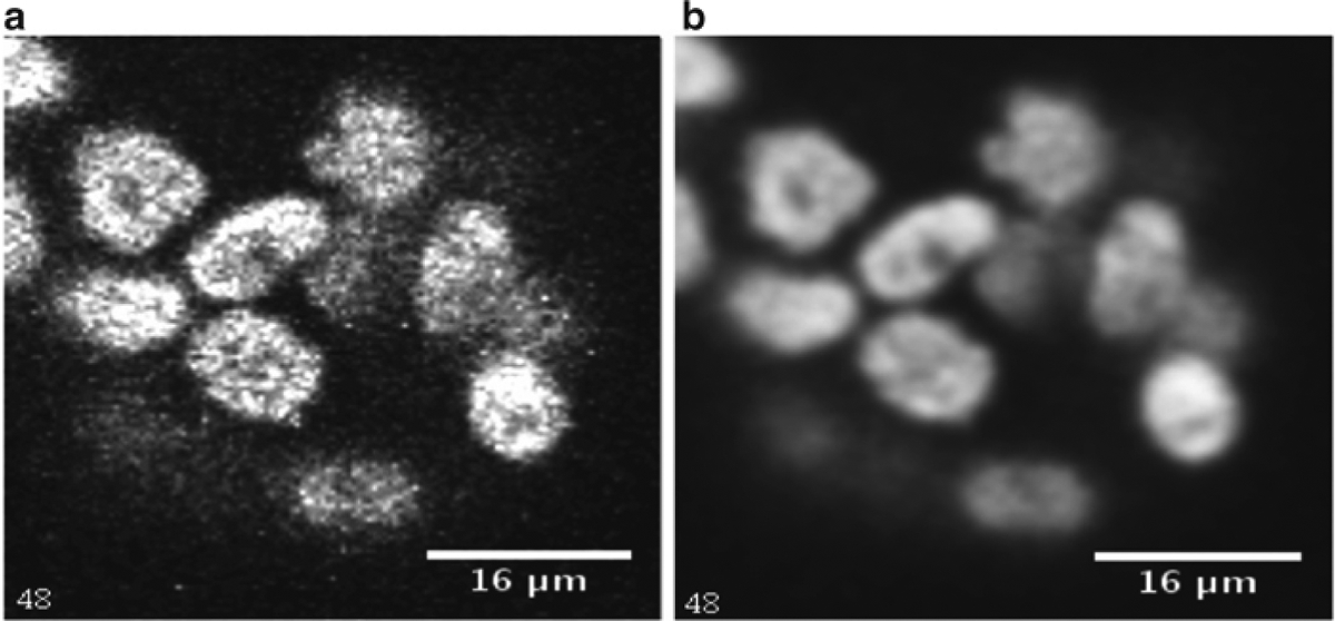
A single slice before and after denoising. (a) Original slice from the MCF-10A sample. (b) Denoised version of A using a Gaussian filter radius of 2.5

Fig. 3.

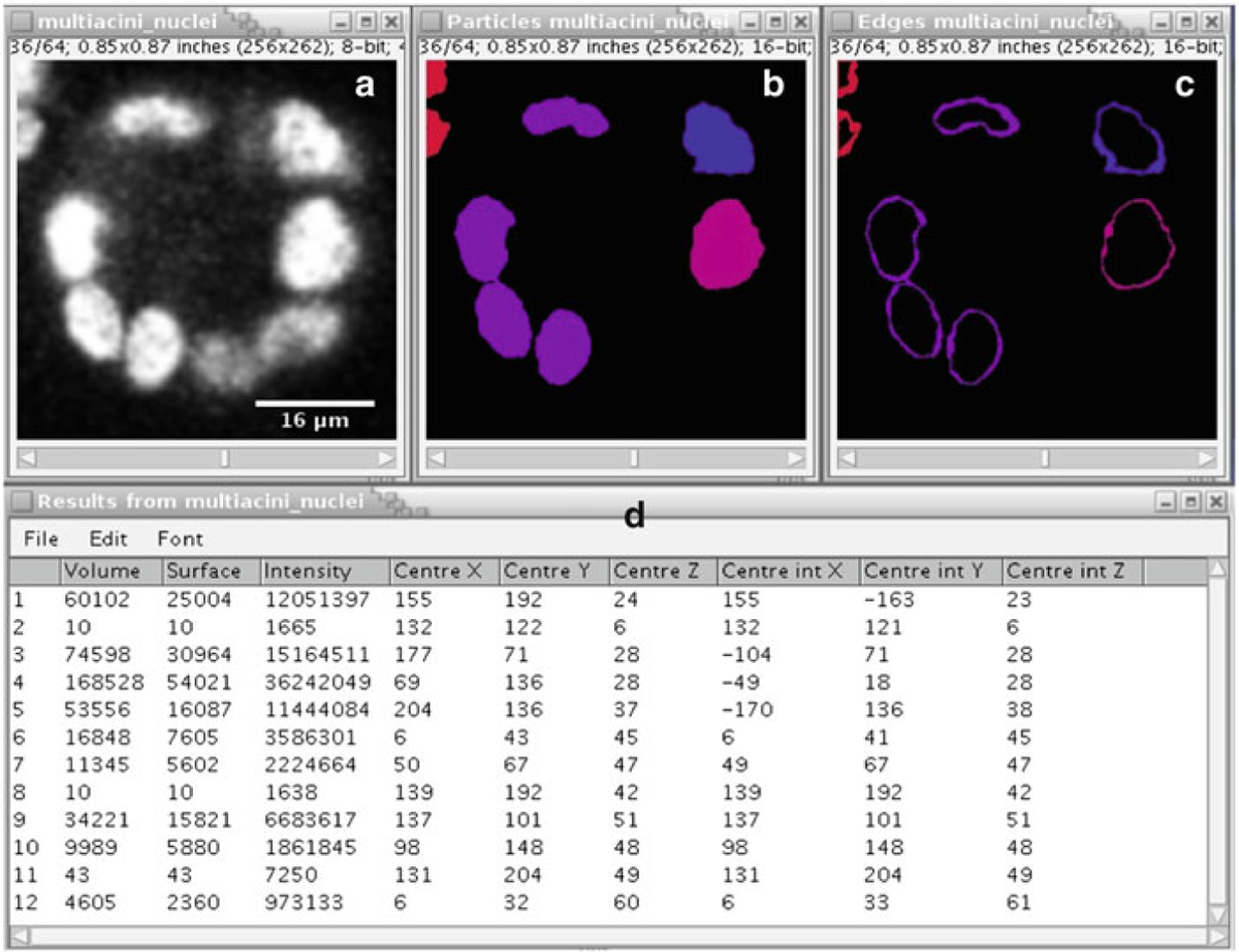
ImageJ output. (a) Original slice from the MCF-10A sample. (b) Detected objects shown in slice 36 using the 3D Object Counter plugin. (c) Edge delineation of the detected samples. (d) Object log showing various statistics obtained from the 3D Object Counter

Note: It is not always possible to segment all the objects successfully using this method since it uses a simple thresholding procedure for the purpose.

3.2. Active Contour Segmentation Using ImageJ

Active contours [11, 12] is an extremely popular modeling method that is used in segmentation and tracking of objects in images and video. It makes use of geometric and probabilistic modeling for analyzing objects. It is far more sophisticated than the previous method since it makes effective use of certain prior information such as local edge strengths and boundary smoothness. However, it processes the image locally instead of using the global information, requiring an initial approximation of the boundary.

The first two steps are the same as the previous procedure. Then we use the ABsnake plugin that uses active contours to calculate the segmentation of a single object across different slices. This plugin will segment one object at a time. The plugin has to be downloaded and installed first.

1. Initialize Snake algorithm: Choose the object to segment and go through the slices to identify the slice range over which it is clearly visible. Go to the first slice in which the object is visible and use the free hand drawing tool (Fig. 1) to draw an approximate boundary for that slice.

2. ABSnake plugin: Go to Plugins > ABSnake. Specify the slices over which the object is clearly visible in the “First slice” and “Last slice” boxes. The “Gradient threshold” value will differ depending upon the image you are going to segment. Choose the color of the boundary and the other options that are available in the plugin window. Once done press “OK.”

3. Output: The output shows the slices with the computed boundaries (Fig. 4). The procedure is then repeated for other nuclei.

Fig. 4.

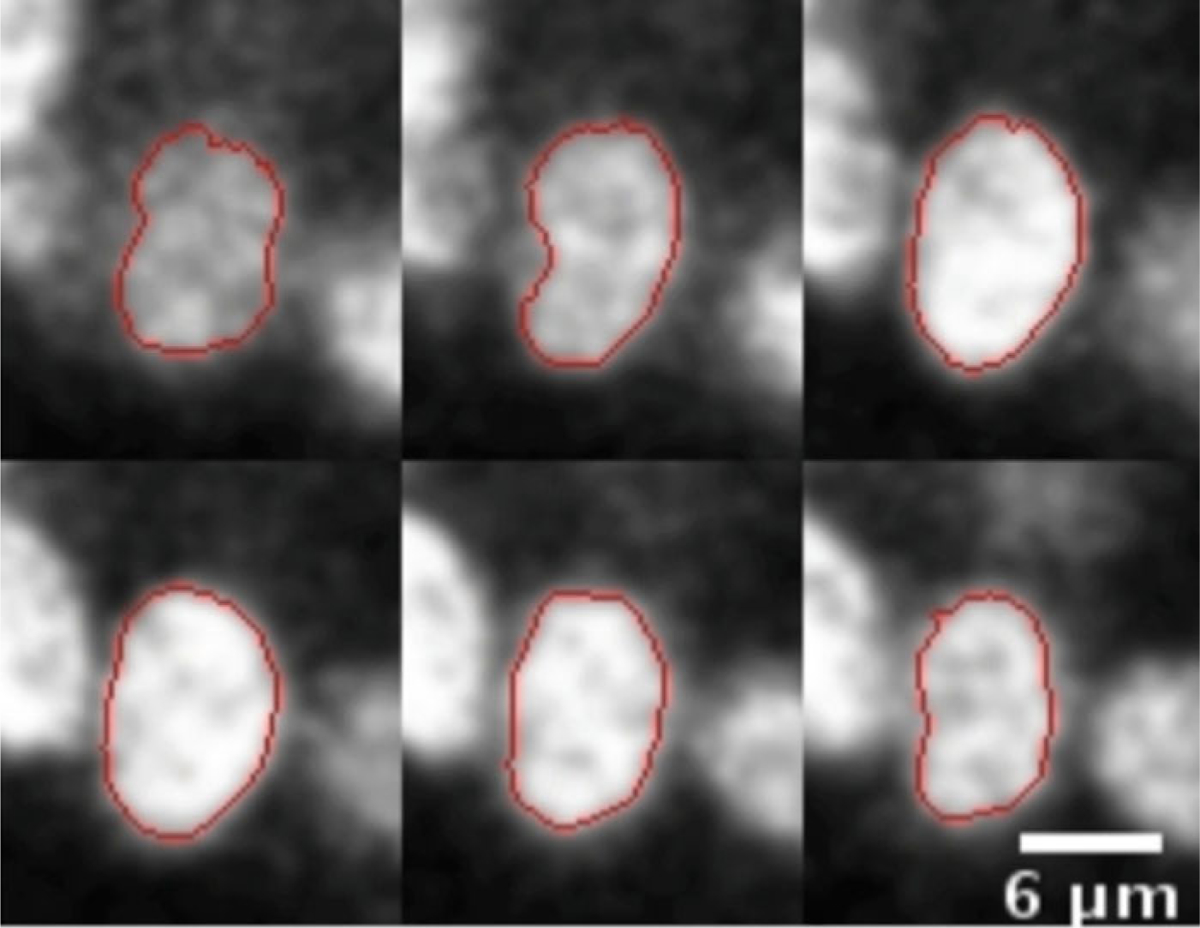
ABSnake plugin. Figure shows six slices out of 12 slices from a sample segmentation of a single nucleus in the MCF-10A sample using the ABSnake plugin in ImageJ

Notes: we have mentioned two different methods for nuclei segmentation using ImageJ. Both of them are somewhat limited in performance, because they segment each 2D slice image independently in a 3D stack image. However, they show good results in most cases. The second method is often sensitive to the initial boundary selection.

4. MIPAV

MIPAV [13] is a general purpose application that is intended for medical and biological microscopic image analysis (Fig. 5). It is also a Java based application and can be used on any Java-enabled platform such as Windows, Unix, or Mac OS X. The main MIPAV site is http://mipav.cit.nih.gov/index.php and it can be downloaded from http://mipav.cit.nih.gov/clickwrap.php. MIPAV can also be extended using plugins and scripts for custom applications. The plugins are functions written in Java using the MIPAV application programming interface (API). The scripts can be recorded using MIPAV and later used on different datasets. MIPAV offers tools for a wide range of operations that can be used for processing images which include filtering, segmentation, measurement and registration. It also has integrated visualization capabilities where one can visualize multidimensional data. The detailed documentation can be obtained at http://mipav.cit.nih.gov/documentation.php.

Fig. 5.

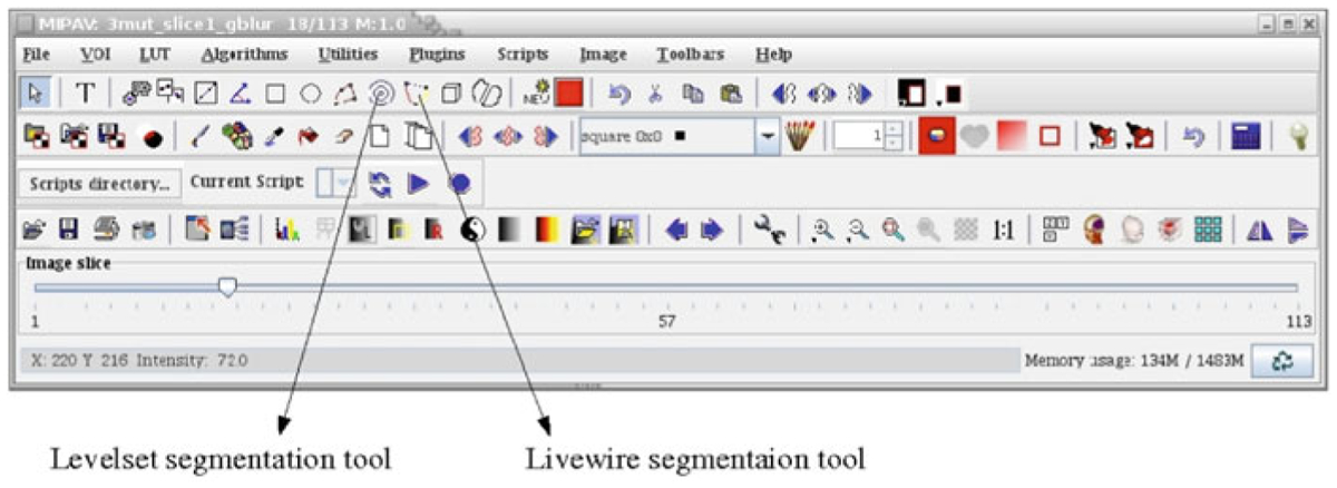
MIPAV GUI indicating the Levelset and Livewire segmentation tools

First we will show 2D segmentation techniques using the Levelset tool and Livewire tool, and then we extend to 3D images. However, for this software the algorithms also analyzed each 2D slice in a 3D stack independently. Tools for segmenting the images using thresholding are also available in this software, but are not described here.

4.1. 2D Method Using the Levelset Tool

1. Reading the image: MIPAV like ImageJ reads a wide variety of image formats. For opening an image go to File > Open Image (A) from disk and select the image that will be analyzed.

2. Blurring to reduce noise: To perform blurring of the image go to Algorithms > Filters (spatial) > Gaussian blur. In the Gaussian blur window choose the degree of blurring necessary by specifying the “Scale of the Gaussian” in X, Y, and Z directions. In the examples presented here, we use 2 for all the dimensions. After choosing all the other options press “OK.”

3. Segmentation using Levelset: Change the slider to change the image slice and choose the slice that is to be segmented. Click on the Levelset tool and position the mouse arrow near the boundary of one of the nuclei to be segmented. This shows a border around the nuclei in yellow. If the border is satisfactory click once and the border color changes to red giving the 2D segmentation for the nucleus (Fig. 6a). If the border shown in yellow is not satisfactory it can be modified by changing the position of the mouse arrow near the border of the nuclei. By repeatedly choosing the Levelset tool all the nuclei in the image slice can be segmented one by one.

Fig. 6.

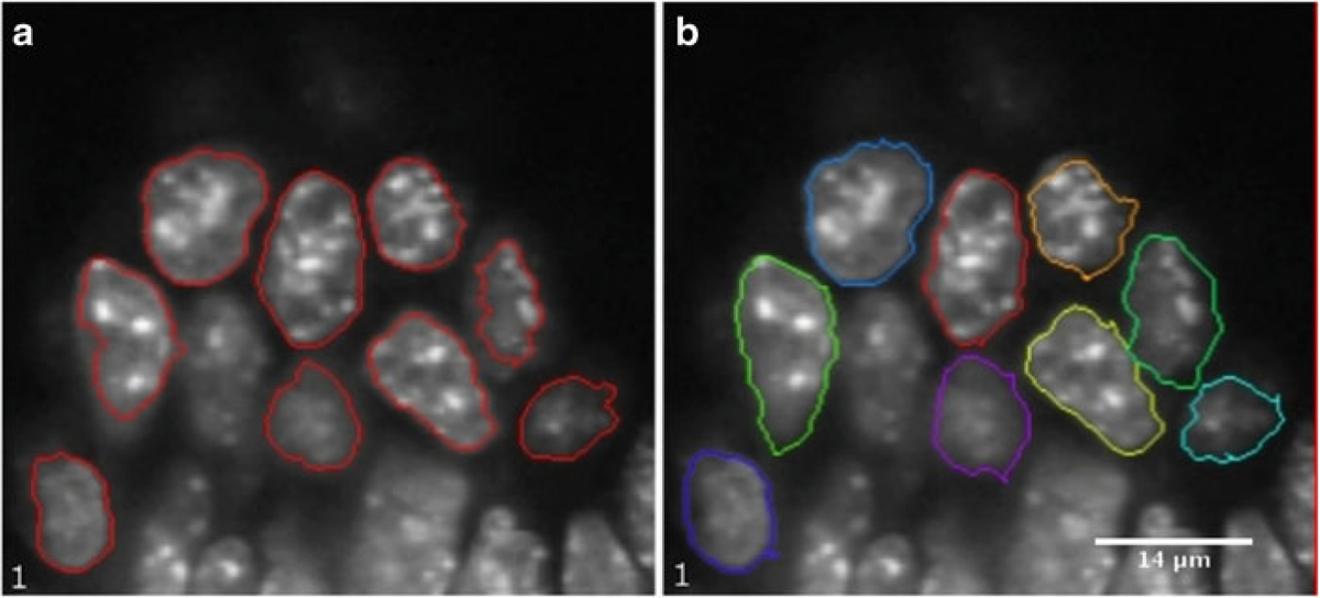
Levelset tool (a) 2D segmentation using the Levelset tool in MIPAV of slice 1 of the somite stage E8.5 mouse embryo image (b) 2D segmentation using Livewire tool in MIPAV of the same sample

4.2. 2D Method Using the Livewire tool

1. Reading the image and performing blurring: Follow steps 1 and 2 mentioned in the previous method (Subheading 4.1).

2. Segmentation using Livewire: Choose the Livewire tool from the MIPAV GUI. This will show a new window where the MIPAV cost function has to be chosen. In case of volume labeled objects such as fluorescent labeled cell nuclei “Gradient magnitude and direction” should be used. On the other hand, when the objects are surface labeled “Intensity” should be used. Since the nuclei in the example are volume labeled we use “Gradient Magnitude and direction”. Press “OK.” Go to the image window and click on a boundary point of the nucleus that is to be segmented first. Move the mouse arrow approximately along the nuclei boundary in a clockwise or anticlock-wise direction. The software will keep on tracing the actual boundary of the nuclei using a dynamic programming (DP) based optimization algorithm [14]. The boundary trace is the path between the first anchor point and the current position of the mouse arrow that has the highest gradient magnitude per voxel compared to any other path between the anchor point and mouse position. To force the boundary to go through a certain point click once to add an anchor point at that location. While tracing around the nuclei keep on adding the anchor points to segment the nuclei satisfactorily. Position the final anchor point near the position of the first anchor point and the boundary will be completed in red. This procedure can be repeated to segment all the nuclei in the slice (Fig. 6b).

4.3. 3D Segmentation Using MIPAV

1. Initialization: For doing 3D segmentation using MIPAV choose an object to be segmented and go through the slices to identify a slice that is approximately in the middle. Perform the 2D segmentation using either one of the tools mentioned namely, Levelset tool or the Livewire.

2. Propagating the boundary to other slices: After 2D segmentation in the previous step, select the contour by clicking on it. Then go to VOI > Evolve boundary 2D > Active contour. In the new window one can specify all the parameters to be used for evolving the boundary. In the “Evolve Boundary” options select “Propagate to adjacent slices” and “Replace Original Contour.” This will propagate the boundary on to the other slices. Press “OK.” After the computation is complete the boundaries of the object in different slices can be viewed by changing the slice number. Usually the algorithm segments in a range of slices adjacent to the starting slice, but omits slices further away from the starting slice even though the object is still visible. In this case the boundary can be propagated further by selecting the last segmentation contours (at the top or bottom) one by one and running the algorithm once more with the same settings.

3. Go to next object: For segmenting the next object, press the new contour button and the GUI will show a new color for the new contour. After this initialization of the new contour follow the steps from 1. In this way all the objects can be segmented.

5. VisSeg

VisSeg is available freely at http://ncifrederick.cancer.gov/Atp/Omal/Flo/. It is a specialized software that is specifically used for semiautomatic 2D and 3D segmentation. It starts with a 2D segmentation of an object in a user selected plane, using DP to locate the border with an average intensity per unit length greater than any other path around the object in that plane. The next step extends the 2D segmentation to the adjacent slices using a combination of DP and combinatorial searching. Once the algorithm has completed the segmentation the user can interactively correct the segmentation by adding anchor points at any location in the 3D-image. The final surface is forced to go through anchor points. The computation algorithms are written in C language and the graphical user interface was developed using Qt (http://qt.digia.com/) and VTK (Visualization Toolkit) (http://www.vtk.org/). For installation of the software one has to install these supporting packages first. The details of the algorithm is available in [15].

General Notes: VisSeg reads images as 8-bit single channel ICS (Image Cytometry Standard) [16]. Some modifications have to be done to the “.ics” file in order to provide all the relevant information to the software. We will cover those in the next section. VisSeg can only accurately segment 3D objects that are point convex. Point convex means that all straight lines radiating in any direction from a user-marked internal point (see below) intersect the boundary of the object exactly once. Point convex objects can contain concavities, but cannot be too irregular in their shape.

Method

1. Conversion and header additions: If necessary use appropriate software, for example MIPAV to convert the image channel that has to be segmented into an 8-bit single channel ICS image. VisSeg requires two more pieces of information to be in the ICS file, the aspect ratio (z-axis-resolution/x[y]-axis-resolution) and the “dyed type” (volume or surface depending on whether the surface is stained or the entire object is stained). Open the “.ics” file using any word processor and add the following lines to the end

   …

   history dyedType volume[or surface]

   history aspectRatio 3.5 [or another number depending on the resolution of the axes]

   …

2. Load the image: Open VisSeg and go to File > Open and choose the ICS image file that has to be segmented. The loaded image will be displayed using volume rendering (Fig. 7a) and in a single slice viewer (Fig. 7b).

3. Data Exploration Controls:

   • In the 3D Rendering Window (Fig. 8a), rotate the image using the mouse left button, pan the image using mouse middle button and zoom using mouse wheel or right button.
   • In 2D Manipulation Window (initially it shows a z-slice) (Fig. 8b), move up and down the z-axis using the mouse middle button, zoom using the mouse wheel or right button outside the big white box and adjust the brightness/contrast using the right button inside the box. One can also rotate the 2D slice using the mouse middle button. To do that, grab the image edge (the red box) using the mouse middle button and rotate. After rotation one can again move up and down the volume using the middle button within the big box. As one rotates the 2D slice the 3D volume rendering window updates and shows the corresponding 2D slice through the volume.
   • The view can be reset to the original view using CTRL+R or go to Edit > Reset Camera.

4. 2D Segmentation: 2D segmentation only works on a “z slice”, an image slice that is orthogonal to the depth axis of the image, so it is better to reset the camera before doing the segmentation. After resetting the camera go to the slice where the nuclei to be segmented is clearly visible. At this point check the “Segmentation Mode” box. Use the mouse left button to mark a point inside the nucleus. Then use the mouse middle button to mark an edge point. The initial 2D segmentation is done immediately after marking the edge point. Correction points can be added using the mouse right button and the updated 2D segmentation is done automatically. The 2D boundary is shown as a red border in the volume rendered image (Fig. 9a) and as a white border in the slice viewer (Fig. 9b).

5. 3D Segmentation: Following 2D segmentation press “Do 3D Seg.” After the 3D segmentation is done the screen will show a surface rendering of the segmented object overlaid on the volume rendering (Fig. 10a) and a white border in the slice viewer (Fig. 10b).

6. 3D Segmentation evaluation windows (Fig. 10c, d): The window in Fig. 10c shows the intensities or gradient magnitude from the original image over the entire surface of the 3D segmented object in a single view known as the “global” view. The white regions suggest a good segmentation, while the dark regions show places where the segmentation is possibly wrong and might need manual correction. One can switch between the original intensity values or gradient magnitude values using the radio buttons in the bottom left corner. The gradient image is only used when the object is volume labeled, as is in this example. When the object is surface stained the original image itself is used instead of the gradient image.

7. Evaluation: Move the mouse pointer over the evaluation window (Fig. 10c) with the right button pressed. The corresponding 2D slice of the original or the gradient image is shown in the 3D segmentation correction window (Fig. 10d) overlaying the original image and the border of the segmented object. This view clearly shows any deviations between the visually observed object surface and the segmented surface.

8. Correction: The red closed path in the 3D segmentation correction window (Fig. 10d) shows the current segmentation result. If the result is not satisfactory, one can add correction points in this window using the mouse right button so that the final segmentation goes through those points. Any number of correction points can be added. After marking the correction points, press “Do 3D Seg” to correct the 3D segmentation. Figure 11 shows full or partial segmentation of the two samples.

9. Undo: During the segmentation process one can undo the current segmentation using CTRL+U or Edit > Undo. This will sequentially delete the result in a decreasing order of object id.

10. Load and Save Segmentation: While performing the segmentation one can save the segmentation done until that point of time by pressing “Save Seg.” The segmentation will be saved as BASE_FILE_NAME.seg file. At a later time the user can load this segmentation and continue segmenting it. To do this first load the original image and then press “Load Seg.”

Fig. 7.

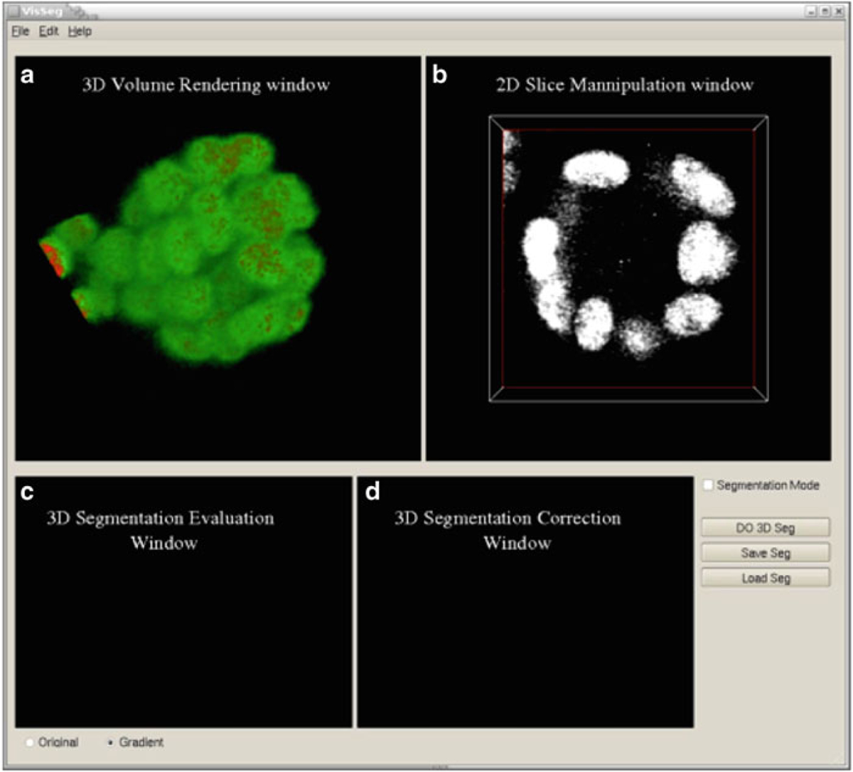
Loading the image in VisSeg. (a) Initial VisSeg GUI 3D volume rendering window showing a MCF-10A sample with nuclear staining. (b) 2D slice manipulation window. (c) 3D segmentation evaluation window. (d) 3D segmentation correction window (refer to Fig. 10c, d for explanations)

Fig. 8.

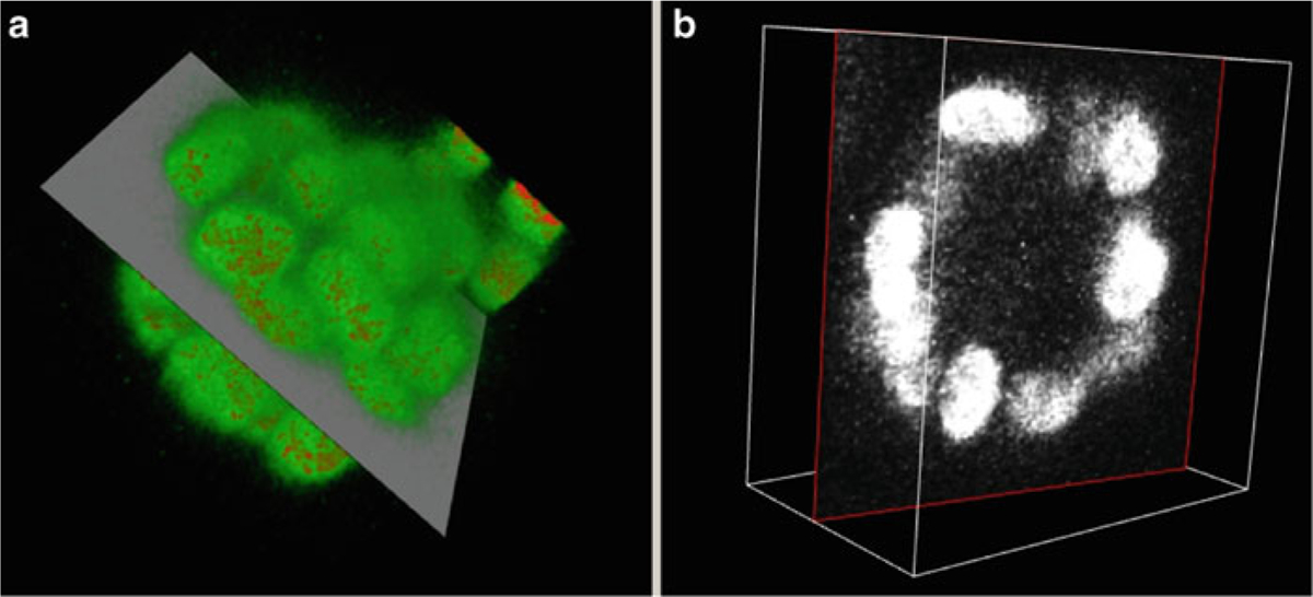
The 3D rendering window and the 2D manipulation window. (a) View of the volume rendering of the nuclear stained MCF-10A sample after view manipulation and showing a 2D plane of view (b) 2D slice manipulation window showing the corresponding 2D plane

Fig. 9.

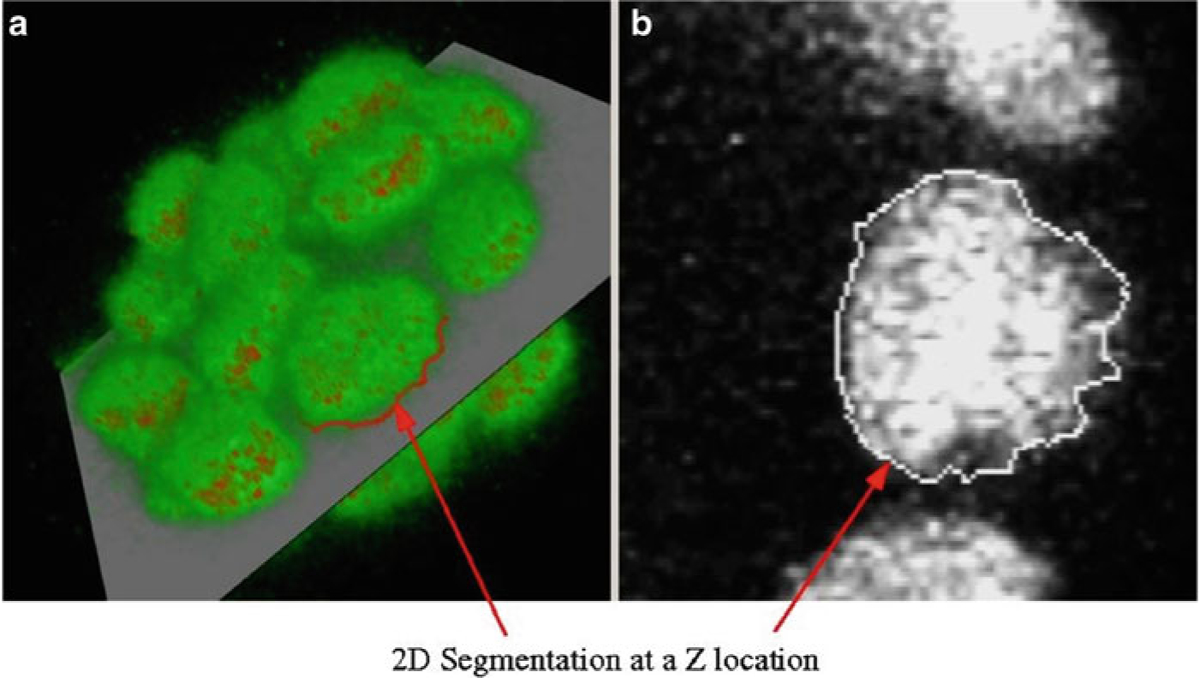
2D segmentation. (a) 2D segmentation of one of the nuclei as viewed in the 3D manipulation window. (b) The boundary is shown in a single Z-slice in the 2D slice manipulation window for the MCF-10A sample

Fig. 10.

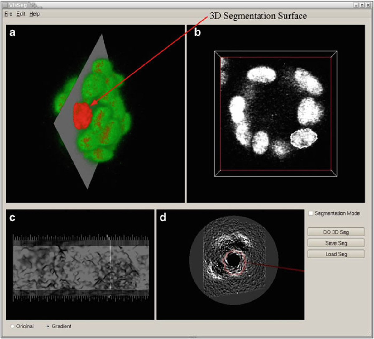
3D Segmentation. (a VisSeg 3D volume rendering window showing the segmentation surface after completion of 3D segmentation of a nuclei. (b) 2D slice showing the 2D segmentation in a specific slice. (c) 3D segmentation evaluation window showing the segmentation quality. (d) 3D segmentation correction window where additional correction points can be added

Fig. 11.

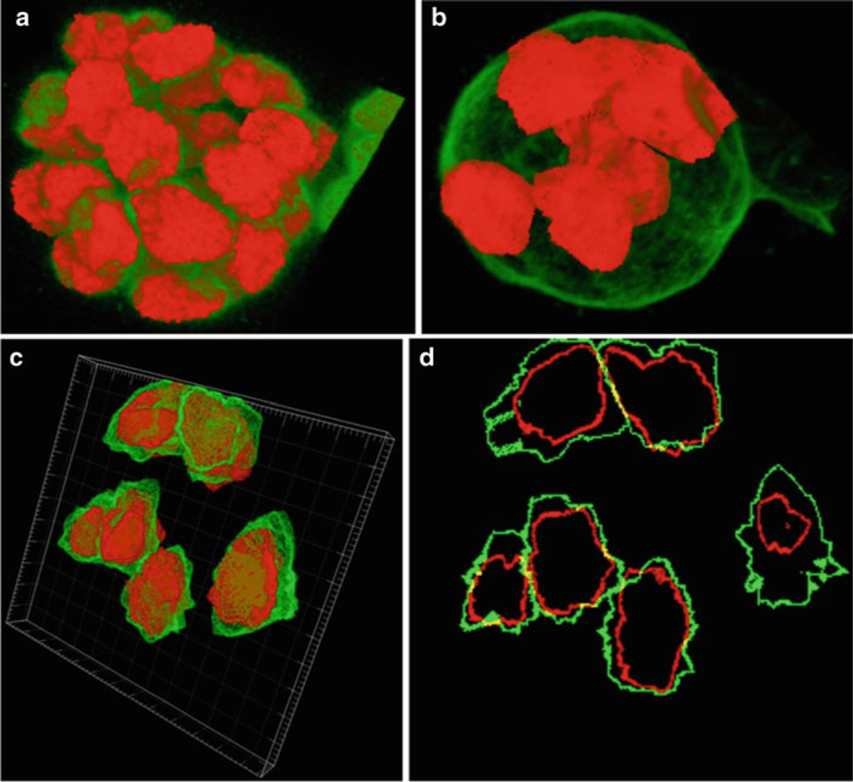
Segmentation correction. (a) Segmentation of all nuclei in the MCF-10A sample using volume staining channel. (b) Partial segmentation of whole cells in the MCF-10A sample using surface staining channel. (c) Partial segmentation of the somite stage mouse embryo sample with surface staining visualized with Imaris (http://www.bitplane.com/go/products/imaris). (d) Slice 13 of the mouse embryo sample showing the nuclear (red) and surface (green) segmentation

6. Concluding Remarks

This chapter illustrates methods and related software for segmentation of individual cells and cell nuclei in developmental tissues. The first two software packages, namely, ImageJ and MIPAV are extremely versatile and offer various image processing and analyzing tools. Although only the relevant portions have been covered here they can be used for a number of other applications. VisSeg on the other hand is a specialized software package which can perform highly accurate and reliable 2D and 3D segmentation of cells and cell nuclei in images with volume or surface fluorescence staining. Segmentation is the starting point for most of the quantitative analysis methods and the methods illustrated in this chapter is a good starting point for such an analysis. Although many other segmentation methods are available we have covered some of the most common and effective ways for segmenting objects in biological images. This kind of quantitative analysis will surely help in gathering more information about complex biological processes.

Appendix

Sample preparation and image acquisition.

Two biological samples were used in this study. One was an early somite stage (E8.0–8.5) mouse embryo obtained from an NIH Swiss female mouse. The embryo was fixed with 2 % paraformaldehyde/phosphate buffered saline (PBS) for 30 min at room temperature and stained with Oregon Green 488 Phalloidin (O-7466, Molecular Probes, Eugene, OR, USA) after treatment with 0.1 M glycine/0.2 % Triton X-100/PBS for 10 min. Phalloidin predominantly labels filamentous actin found abundantly at the cell surface underlying the cell membrane. The embryo was counter stained with the DNA dye 4′,6-diamidino-2–phenylindole (DAPI). The posterior primitive streak region of the embryos was manually dissected and mounted with SlowFade Light Antifade kit (S-7461, Molecular Probes) on a glass slide. Images were acquired using a 40×, 1.3 numerical aperture oil objective lens, and pinhole of one airy unit on an LSM 510 confocal microscope (Carl Zeiss Inc., Thornwood, NY, USA). Excitation was with a 488-nm laser light and emitted light between 500 and 550 nm was acquired. Thus, the effective thickness of the optical sections was 425 nm at the coverslip but increased further away from the coverslip. Pixel size was 0.14 μm in the x and y dimensions. DAPI was excited with two photon excitation at 780 nm and emitted light between 420 and 480 nm was collected.

The other biological sample used in this chapter was a 3D cell culture model of early breast tumorigenesis. MCF-10A.B2 a human mammary epithelial cell line was grown on basement membrane extract (Trevigen Inc., Gaithersburg, MD) for 20 days. MCF-10A. B2 cells express a synthetic ligand-inducible active ErbB2 variant. To induce tumorigenesis the synthetic ligand (AP1510; ARIAD Pharmaceuticals Inc)) was added for the final 10 days of culture. The acini structures formed by growth in 3D culture were fixed in 2 % paraformaldehyde/PBS for 20 min at room temperature and permeabilized by a 10 min incubation in 0.5 % Triton X-100 at 4 °C. Following three 15 min rinses in 100 mM glycine/PBS, the acini were blocked in IF buffer (0.1 % bovine serum albumin/0.2 % Triton X-100/0.05 % Tween-20/PBS) containing 10 % fetal bovine serum (Invitrogen) for 1 h. The cells were then incubated overnight in anti-integrin alpha 6 antibody (Chemicon International). Integrin alpha 6 stains for basolateral polarity, it stains the cell surface membrane with strong basal and weaker lateral staining. After three 20 min washes in IF buffer the cells were incubated in Alexa Fluor 488 donkey anti-rat (Invitrogen). Samples were mounted in DAPI containing VECTASHIELD mounting media (Vector Laboratories Ltd.) after three further 20 min washes in IF buffer. Images were acquired using a 63× 1.4- NA oil objective lens on an LSM 510 confocal microscope.

References

- 1.Pawley J (2006) Handbook of biological confocal microscopy, 3rd edn. Springer, New York [Google Scholar]
- 2.Russ JC (2002) The image processing handbook, 4th edn. CRC, Boca Raton, FL [Google Scholar]
- 3.Castleman KR (1995) Digital image processing. Prentice Hall, Englewood Cliffs, NJ [Google Scholar]
- 4.Delft University of Technology, Quantitative Imaging Group interactive image processing course. http://www.tnw.tudelft.nl/fileadmin/Faculteit/TNW/Over_de_faculteit/Afdelingen/Imaging_Science_and_Technology/Research/Research_Groups/Quantitative_Imaging/Education/doc/FIP2_3.pdf
- 5.Merks RMH, Brodsky SV, Goligorksy MS, Newman SA, Glazier JA (2006) Cell elongation is key to in silico replication of in vitro vasculogenesis and subsequent remodeling. Dev Biol 289:44–54 [DOI] [PMC free article] [PubMed] [Google Scholar]
- 6.Heid PJ, Voss E, Soll DR (2002) 3D-DIASemb: a computer-assisted system for reconstructing and motion analyzing in 4D every cell and nucleus in a developing embryo. Dev Biol 245:329–347 [DOI] [PubMed] [Google Scholar]
- 7.Blacher S, Devy L, Burbridge MF, Roland G, Tucker G, Noël A, Foidart J-M (2001) Improved quantification of angiogenesis in the rat aortic ring assay. Angiogenesis 4:133–142 [DOI] [PubMed] [Google Scholar]
- 8.Peng H, Long F, Zhou J, Leung G, Eisen MB, Myers EW (2007) Automatic image analysis for gene expression patterns of fly embryos. BMC Cell Biol 8(Suppl 1):S7. [DOI] [PMC free article] [PubMed] [Google Scholar]
- 9.ImageJ website. http://rsb.info.nih.gov/ij/
- 10.MIPAV website. http://mipav.cit.nih.gov/index.php.
- 11.Kass M, Witkin A, Terzopoulos D (1988) Snakes: active contour models. Int J Comput Vision 1:321–331 [Google Scholar]
- 12.Blake A, Isard M (1998) Active contours. Cambridge University Press, New York, NY [Google Scholar]
- 13.McAuliffe MJ, Lalonde FM, McGarry D, Gandler W, Csaky K, Trus BL (2001) Medical image processing, analysis and visualization in clinical research. Proceedings 14th IEEE symposium on computer-based medical systems, pp 381–386 [Google Scholar]
- 14.Baggett D, Nakaya M, McAuliffe M, Yamaguchi TP, Lockett S (2005) Whole cell segmentation in solid tissue sections. Cytometry A 67A: 137–143 [DOI] [PubMed] [Google Scholar]
- 15.McCullough DP, Gudla PR, Harris BS, Collins JA, Meaburn KJ, Nakaya M, Yamaguchi TP, Misteli T, Lockett SJ (2008) Segmentation of whole cells and cell nuclei from 3D optical microscope images using dynamic programming. IEEE Trans Med Imaging 27:723–734 [DOI] [PMC free article] [PubMed] [Google Scholar]
- 16.Dean P, Mascio L, Ow D, Sudar D, Mullikin J (1990) Proposed standard for image cytometry data files. Cytometry 11:561–569 [DOI] [PubMed] [Google Scholar]